Threshold Probability Functions and
Thermal Inhomogeneities in the Lyman-alpha Forest

Abstract

We introduce to astrophysics the threshold probability functions $S_{2}$,$C_{2}$, and $D_{2}$ first derived by Torquato et al. (1988), which effectively samples the flux probability distribution (PDF) of the Ly$\alpha$ forest at different spatial scales. These statistics are tested on mock Ly$\alpha$ forest spectra based on various toy models for He II reionization, with homogeneous models with various temperature-density relations as well as models with temperature inhomogeneities. These mock samples have systematics and noise added to simulate the latest Sloan Digital Sky Survey Data Release 7 (SDSS DR7) data. We find that the flux PDF from SDSS DR7 can be used to constrain the temperature-density relation $\gamma$ (where $T\propto(1+\Delta)^{\gamma-1}$) of the intergalactic medium (IGM) at $z=2.5$ to a precision of $\Delta\gamma=0.2$ at $\sim 4\sigma$ confidence. The flux PDF is degenerate to temperature inhomogeneities in the IGM arising from He II reionization, but we find $S_{2}$ can detect these inhomogeneities at $\sim 3\sigma$, with the assumption that the flux continuum of the Ly$\alpha$ forest can be determined to 9% accuracy, approximately the error from current fitting methods. If the flux continuum can be determined to 3% accuracy, then $S_{2}$ is capable of constraining the characteristic scale of temperature inhomogeneities, with $\sim 4\sigma$ differentiation between toy models with hot bubble radii of 50 $\,h^{-1}\,\mathrm{Mpc}$ and 25 $\,h^{-1}\,\mathrm{Mpc}$.

1. Introduction

The absorption of radiation by the Lyman-$\alpha$ (Ly$\alpha$) resonance of neutral hydrogen along the line-of-sight to high-redshift quasars, commonly known as the Ly$\alpha$ forest, is an important probe of large-scale structure at $z\gtrsim 2$ (see, e.g., Croft et al. 1998; McDonald et al. 2000; Croft et al. 2002; Zaldarriaga et al. 2003; McDonald et al. 2005). The utility of the Ly$\alpha$ forest as a cosmological tool has been enabled by theoretical work on the intergalactic medium (IGM) (see, e.g., Cen et al. 1994; Miralda-Escudé et al. 1996; Croft et al. 1998; Davé et al. 1999; Theuns et al. 1998), which allowed the underlying dark matter field to be mapped from the Ly$\alpha$ absorption.

In recent years, increasing attention has been turned towards obtaining a deeper understanding on the detailed astrophysics of the IGM such as the ionizing ultraviolet background, temperature field, metals, etc. The reionizations of H I and He II have been shown to play critical roles in regulating the properties of the IGM.

The reionization of He II at $z\sim 3$ should leave an observable imprint on the properties of the Ly$\alpha$ forest. Recent theoretical developments have recognized that He II reionization must have occurred in an extended and inhomogeneous fashion as the process was driven by rare and bright quasars (Lai et al. 2006; Furlanetto & Oh 2008b; McQuinn et al. 2009). These spatial variations in He II reionization history should modulate the equation of state and entropy of the IGM.

Observations of the Ly$\alpha$ forest have the potential to reveal details of this reionization process. The sources of $E>54.4\mathrm{eV}$ photons which drive He II reionization are believed to be rare bright quasars, but different model assumptions on, e.g., quasar duty cycles and luminosity functions can dramatically change the history and morphology of He II reionization (McQuinn et al. 2009), as well as the thermal properties of the resulting IGM (Furlanetto & Oh 2008a).

Observational constraints on He II reionization have arguably lagged behind the theoretical work. Schaye et al. (2000) measured a peak at $z\approx 3$ in the temperature evolution of the IGM from the Doppler parameters of high-resolution Ly$\alpha$ forest spectra, that they claimed to be due to He II reionization. While some authors (Theuns et al. 2002; Bernardi et al. 2003; Faucher-Giguère et al. 2008) argue that the detection of the feature at $z\sim 3.2$ in the evolution of the effective Ly$\alpha$ optical depth, $\tau_{\mathrm{eff}}$, of the IGM provides further evidence for the reionization transition, Dall’Aglio et al. (2009) failed to find this transition. More recently, the Cosmic Origins Spectrograph on the Hubble Space Telescope is beginning to shed light on He II reionization through studies of the He II Ly$\alpha$ forest and associated He II Gunn-Peterson troughs (see, e.g., Shull et al. 2010).

Measurements of the flux probability distribution function (PDF Jenkins & Ostriker 1991) of high-resolution Ly$\alpha$ forest spectra (e.g., McDonald et al. 2000; Lidz et al. 2006; Kim et al. 2007) have constrained the equation of state $\gamma$ of the IGM. In this paper, we define the equation of state of the gas as a function only of the gas density:

$$T(\Delta)=\bar{T}\;\Delta^{\gamma-1},$$ (1)

where $T(\Delta)$ is the temperature as a function of density, $\bar{T}$ is the temperature at mean density, and $\Delta=\rho/\langle\rho\rangle$ is the density contrast of the gas. Different scenarios for He II reionization make distinctive predictions for the redshift evolution of $\gamma$. Several authors (Becker et al. 2007; Viel et al. 2009) claimed to have detected an inverted equation of state $\gamma<1$, which is has been theorized to arise from the late reionization of voids (Furlanetto & Oh 2008a). Lidz et al. (2009) attempted to measure spatial inhomogeneities in the thermal state of the IGM by using a wavelet filter on high-resolution spectra, but had a null detection.

Most observational attempts to place constraints on the IGM have been based on relatively small-numbers of high-resolution ($R\equiv\lambda/\Delta\lambda\sim 10^{4}$) and high signal-to-noise ($\mathrm{S/N}\sim 10^{2}$ per pixel) spectra. However, the largest single source of data on the Ly$\alpha$ forest is arguably the Sloan Digital Sky Survey (York et al. 2000), which includes $\sim 10^{4}$ quasars with useable Ly$\alpha$ forest, albeit of moderate quality ($R\approx 2000$, $\mathrm{S/N}\sim 4$). In the near future, the Baryon Oscillation Spectroscopic Survey (BOSS, part of SDSS-III) aims to increase the sample size of high-redshift ($z\gtrsim 2$) quasars to $\gtrsim 10^{5}$ at a similar spectral resolution to the SDSS.

Many of the techniques (Voight profile fitting, wavelet analysis etc.) developed for probing the IGM are unsuitable for use with the lower quality of the SDSS data, while the flux statistics that have been measured for the SDSS Ly$\alpha$ forest, such as the flux power spectrum, are relatively insensitive to the detailed astrophysics of the IGM. For example, Lai et al. (2006) have shown that the SDSS flux power spectrum is insensitive to large-scale temperature inhomogeneities arising from He II reionization.

In this paper, we borrow some statistics used to measure mechanical and transport properties of disordered media in the material sciences, which we term the ‘threshold probability functions’, and explore their applications to mock Ly$\alpha$ forest spectra based on the SDSS sample. We will generate simple toy models for the IGM based on different scenarios for He II reionization, and explore the ability of the threshold probability functions to distinguish between them.

We first introduce and define these statistics in §2, before digressing to discuss the simulations and toy models we use to generate the mock spectra in §3. In §4 we calculate the flux PDF as a check on our errors, before going on to apply the threshold statistics on the mock data in §5.

2. Definition of Threshold Statistics:
$S_{2}$, $C_{2}$, and $D_{2}$

In the study of the Ly$\alpha$ forest, the two-point flux correlation function is commonly defined as:

$$\xi(r)=\langle\delta_{F}(r^{\prime})\>\delta_{F}^{*}(r^{\prime}+r)\rangle,$$ (2)

where $r$ is the comoving distance between two points in the line-of-sight of the background quasar (equivalently expressed as redshift, wavelength, or velocity intervals within the observed spectrum), and

$$\delta_{F}(r)=\frac{F(r)}{\bar{F}}-1$$ (3)

where $F(r)=e^{-\tau(r)}$ is the flux transmitted through the Ly$\alpha$ optical depth $\tau(r)$ at a given point, and $\bar{F}$ is the mean transmitted flux in the spectrum. Another commonly used statistic is the Fourier transform of $\xi_{F}(r)$, the flux power spectrum

$$P_{F}(k)=\int^{\Delta r/2}_{-\Delta r/2}\xi_{F}(r^{\prime})e^{ikr^{\prime}}dr^{\prime}$$ (4)

computed over the interval $\Delta r$, and $k$ is the wavenumber.

In this paper we introduce to astrophysics several related two-point statistics used in material science (Torquato et al. 1988; Jiao et al. 2009). For a volume that is occupied by a two-phase medium, for any one of the phases (say phase $i$) we can define

$$\hat{S}_{2}(\vec{r_{1}},\vec{r_{2}})=\hat{C}_{2}(\vec{r_{1}},\vec{r_{2}})+\hat{D}_{2}(\vec{r_{1}},\vec{r_{2}}).$$ (5)

$\hat{S}_{2}$ is the probability function of finding both points $\vec{r_{1}}$ and $\vec{r_{2}}$ in phase $i$, while $\hat{C}_{2}$ and $\hat{D}_{2}$ denote the probability of finding points of the phase $i$ within the same ‘cluster’ (in this paper referring to contiguous groupings of pixels, not galaxy or star clusters), and in separate clusters, respectively. This is illustrated in Figure 1. $\hat{C}_{2}$, known as the ‘cluster function’, encodes higher-order not contained in two-point statistics (Jiao et al. 2009). For astrophysical purposes we assume an isotropic and homogeneous field, so $\hat{S}_{2}(\vec{r_{1}},\vec{r_{2}})=\hat{S}_{2}(|\vec{r_{1}}-\vec{r_{2}}|)=\hat{S}_{2}(r)$ etc.

We generalize these statistics for use with the Ly$\alpha$ forest by defining them as a function of flux threshold, $F_{th}$. At each value of $F_{th}$, we divide the spectrum into high ($F>F_{th}$) and low ($F<F_{th}$) regions and then compute the clustering properties for these phases. In this paper we focus on the high ($F>F_{th}$) phases which are more sensitive to He II reionization. This defines two dimensional functions, $\hat{S}_{2}(r,F_{th})$, $\hat{C}_{2}(r,F_{th})$, and $\hat{D}_{2}(r,F_{th})$.

Figure 1.— A segment of transmitted Ly$\alpha$ forest flux plotted as a function of comoving distance $r$ along the line-of-sight, illustrating the definition of the threshold probability functions $\hat{C}_{2}$ and $\hat{D}_{2}$. All pixels above the flux threshold ($F_{th}=0.75$ in this example) contribute to $\hat{C}_{2}$, $\hat{D}_{2}$, and $\hat{S}_{2}\equiv\hat{C}_{2}+\hat{D}_{2}$. The arrows at left illustrate a pixel pair within the same ‘cluster’ of pixels which contribute to $\hat{C}_{2}$, while the arrows at right denote another pixel pair in different clusters which contribute to $\hat{D}_{2}$.

The threshold probability function at zero lag, $\hat{S}_{2}(0|F_{th})$ is directly related to the familiar flux probability distribution function (PDF), $p(F)$:

$$\hat{S}_{2}(0|F_{th})=\int^{1}_{F_{th}}p(F)dF.$$ (6)

The number of possible pixel pairs (and hence $\hat{S}_{2}$) decreases linearly with $r$ within a finite length $L$. In order to take this effect into account we introduce a rescaled version of $\hat{S}_{2}$:

$${S_{2}}(r|F_{th})=\hat{S}_{2}(r|F_{th})\left(1-\frac{r}{L}\right),$$ (7)

and similarly for $\hat{C}_{2}$ and $\hat{D}_{2}$. At large separations, $S_{2}(r|F_{th})\rightarrow S^{2}_{2}(0|F_{th})$ if there is no large-scale order in the system. We refer to $S_{2}(r|F_{th})$, $C_{2}(r|F_{th})$, and $D_{2}(r|F_{th})$ collectively as the ‘threshold probability functions’. Intuitively, they can be thought of as the flux PDF evaluated as a function of correlation length.

These threshold probability functions should not be confused with the threshold crossing statistics that counts the number of times that the observed Ly$\alpha$ forest transmission spectrum intersects a given flux value per unit redshift (Miralda-Escudé et al. 1996; Fan et al. 2002). The threshold crossing statistic is a generalization of the forest line density and does not contain spatial information, unlike the threshold probability functions.

While He II reionization may create a two-phase thermal structure in the IGM (Lai et al. 2006; McQuinn et al. 2009), its imprint on the Ly$\alpha$ forest will not be manifested as distinct phases in the flux distribution of the Ly$\alpha$ forest spectra. It is the density field which predominantly determines the distribution of low- and high-absorption regions. These thermal inhomogeneities, however, do modulate the amplitude of the optical depth and leave a potentially statistically detectable effect especially in the low-absorption regions. It is this effect which we are attempting to detect using the threshold clustering functions.

3. Ly$\alpha$ Forest Model

In this section, we describe a series of simulations of the Ly$\alpha$ forest that we will use to test ability of the threshold probability functions to distinguish between different He II reionization histories.

3.1. Simulations

We use a set of publicly available mock Ly$\alpha$ forest spectra (Slosar et al. 2009) that have been generated from dark matter-only particle-mesh simulations based on a flat $\Lambda$CDM cosmology with $\Omega_{\Lambda}=0.75,\Omega_{M}=0.25,h=0.75,n=0.97,$ and $\sigma_{8}=0.8$. The simulations evolved $3000^{3}$ particles in a $1500\,h^{-1}\,\mathrm{Mpc}$ box with the forces computed on a $3000^{3}$ grid. Density and velocity fields were then generated using spline-kernel interpolation with an effective smoothing radius of $250\,h^{-1}\,\mathrm{kpc}$, and line-of-sight skewers extracted at redshift $z=2.5$ with a spacing of $10\,h^{-1}\,\mathrm{Mpc}$ to provide $150^{2}=22500$ skewers from each run.

The Ly$\alpha$ optical depth in each pixel was then generated using the fluctuating Gunn-Peterson approximation (FGPA, Croft et al. 1998; Gnedin & Hui 1998a):

$$\tau\propto\bar{T}^{-0.7}\Delta^{2-0.7(\gamma-1)}\left(1+\frac{1}{H(z)}\frac{dv_{pec}}{dx}\right),$$ (8)

where $\Delta=\rho/\bar{\rho}$ is the density perturbation, $H(z)$ is the Hubble parameter at redshift $z$, ${dv_{pec}/dx}$ is the peculiar velocity gradient, $\bar{T}$ is the temperature at mean density, and $\gamma$ parametrizes the equation of state between density and temperature (see Equation 1). In these runs $\bar{T}=2\times 10^{4}K$ and $\gamma=1.5$ was assumed. In addition to the optical depth skewers, matching skewers of the underlying density were also made available.

These dark matter simulations are not expected to accurately capture the small-scale power of the Ly$\alpha$ forest as hydrodynamics are not included. However, they provide a fiducial set of mock spectra from which it is easy to generate different toy models of the IGM by adjusting the optical depths using the FGPA (Eq. 8). This provides a convenient testing ground for the ability of the threshold probability functions to distinguish between differences arising from different IGM models.

3.2. Homogeneous IGM Models

The fiducial set of simulated spectra described above assumes a homogeneous IGM in which $\bar{T}=2\times 10^{4}K$ and $\gamma=1.5$. This is the value of $\gamma$ at which unshocked gas settles at $z\sim 3$ after a hydrogen reionization event at $z\gtrsim 6$ (Hui & Gnedin 1997), while $\bar{T}=2\times 10^{4}K$ is approximately the value obtained through line-profile fitting of high-resolution Ly$\alpha$ forest spectra (McDonald et al. 2001; Theuns et al. 2002). We refer to this fiducial model as ‘G1.5’.

We study the effects of changing the equation of state uniformly across the IGM by creating models with $\gamma$ set to 1.3 and 0.8 (models G1.3 and G0.8, respectively). $\gamma=0.8$ represents an inverted equation of state predicted by Furlanetto & Oh (2008a) for scenarios in which dense regions, which were reionized early on, have had time to cool adiabatically to temperatures lower than more recently reionized voids. We introduce G1.3 as an intermediate case between G1.5 and G0.8, although as we shall see later, it has a flux PDF which is degenerate with our inhomogeneous reionization models.

The mean temperature $\bar{T}$ is kept unchanged, as global variations in temperature will be manifested as changes in the mean flux level, which we regard as a fixed parameter by normalizing our Ly$\alpha$ forest spectra to the same value of $\langle F\rangle=0.8$ (Meiksin & White 2004).

3.3. Inhomogeneous IGM Models

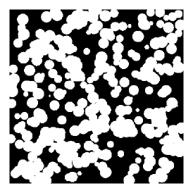
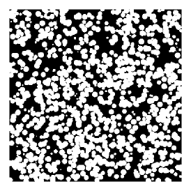
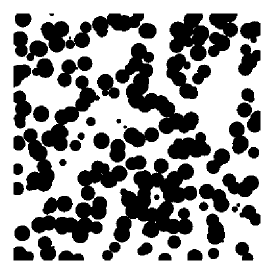
Figure 2.— Examples of pixel masks used to generate the inhomogeneous IGM models, shown here as 2-dimensional cross-sections across the box which is 1500 $\,h^{-1}\,\mathrm{Mpc}$ on a side. From left to right: Models R50, R25, and I50. White represents the hot IGM phase while black is the cold phase with both occupying 50% of the volume. The mock spectra will thus represent 1-dimensional samplings through the hot and cold phases shown here.

Several authors (Lai et al. 2006; McQuinn et al. 2009) have suggested that the reionization of He II by quasars at $z\sim 3$ results an inhomogeneous IGM with significantly heated regions. In this paper we consider a basic picture of inhomogeneous He II reionization inspired by the simulation results of McQuinn et al. (2009), in which the IGM is composed of hot and cold phases with equal volume-filling factors of 50% each. The hot phase has a mean temperature $\bar{T}_{h}=2.5\times 10^{4}K$ and $\gamma=1.2$, while the cold phase has a mean temperature $\bar{T}_{c}=1.5\times 10^{4}K$ and $\gamma=1.5$. Note that while changes in the overall mean temperature will be absorbed in the mean flux level, the contrast between $\bar{T}_{h}$ and $\bar{T}_{c}$ is more important as it results in relative changes of optical depth independent of the overall flux normalization.

We approximate the spatial distribution of the hot and cold regions by generating a pixel mask in which bubbles of radius $R_{bub}$ are randomly inserted into a 3-dimensional box with a comoving volume $(1500\,h^{-1}\,\mathrm{Mpc})^{3}$, the same size as the simulation box. These bubbles, which are allowed to overlap, are added until 50% of the volume lies within bubbles. This allows a full distribution of intersection path lengths within the mock spectra, from close to zero to several times $R_{bub}$ as illustrated in Figure 2. Our simple model provides a simulacrum of the complex spatial morphologies seen in McQuinn et al. (2009). Note that we neglect peculiar velocities as the bubble positions are completely random and have no overall correlations with large scale-structure.

The mock spectra from the simulations are then modified on a pixel-by-pixel basis depending on whether the three-dimensional spatial position of each pixel was flagged by the pixel mask: the optical depths of pixels which fall within hot bubbles are rescaled using the FGPA (Equation 8) so that they have $\bar{T}=\bar{T}_{h}$ and $\gamma=1.2$, while pixels outside the bubbles have $\bar{T}=\bar{T}_{c}$ and $\gamma=1.5$. Note that this does not take into account the effect of thermal broadening. Although thermal broadening primarily affects the small-scale power of the forest, it also has a small effect on the large-scale bias. This coupling between the large- and small-scale power is not well-understood and will need to be accounted for in a full data analysis using large-scale hydrodynamical simulations, but for the approximate treatment in this paper we ignore this effect.

The characteristic scale of the thermal inhomogeneities arising from He II reionization are expected to be dependent on quasar physics such as duty cycles, clustering and ionizing spectrum (McQuinn et al. 2009). We thus test the threshold probability functions to this characteristic scale by introducing models with hot bubbles of $R_{bub}=50\,h^{-1}\,\mathrm{Mpc}$ and $R_{bub}=25\,h^{-1}\,\mathrm{Mpc}$, denoted by R50 and R25 respectively. Both these models have the same volume filling fraction of 50% for hot bubbles.

In addition, we created a model, I50, in which the topology of He II reionization is inverted, i.e. the IGM is composed of cold bubbles of $R_{bub}=50\,h^{-1}\,\mathrm{Mpc}$ with the surrounding regions filled with the hot phase, with the properties of the hot and cold phases identical to those of models R50 and R25. Although this model is not physically realistic, we include it to test the sensitivity of the threshold statistics towards topology. Figure 2 illustrates the inhomogeneities in our various models.

All the inhomogeneous models, R50, R25, and I50, have the same total number of pixels intersecting with hot regions when averaged across large numbers of spectra. The differences lie in the manner the pixels are spatially distributed along the skewers.

3.4. Mock Spectra

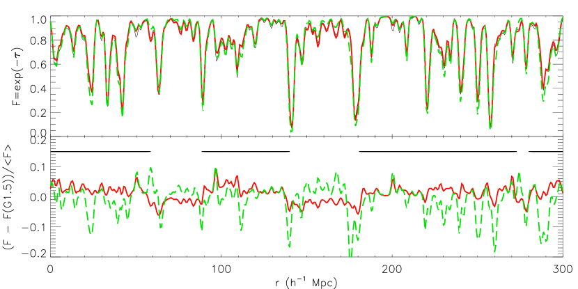
Figure 3.— Top panel: Flux transmission spectra from models G1.5 (thin black line), G0.8 (green dashed line), and R50 (thick red line) for one line-of-sight – shown here without noise or other systematics. Bottom panel: Difference in flux between models G0.8 and G1.5 (green dashed line), and between R50 and G1.5 (solid red line), normalized by the mean flux. The horizontal bars indicate the portions of the line-of-sight which intersect with hot bubbles. See electronic edition of the Journal for a color version of this figure.

As the primary purpose of this paper is to study the ability of the threshold statistics to constrain the IGM using existing SDSS data, in this paper we model the instrumental and systematic effects at an approximate level sufficient to estimate the errors. A more detailed approach is to be deferred to a later data analysis paper.

First, flux transmission spectra are generated from the optical depth skewers from $F=\exp{(-\tau)}$, with a global mean flux set to $\langle F\rangle=0.8$. The spectra are then Gaussian-smoothed to the resolution of the SDSS spectra which have FWHM=$150\,\mathrm{km\;s^{-1}}$ (corresponding to $\simeq 1.4\,h^{-1}\,\mathrm{Mpc}$ at $z=2.5$) and binned into $70\,\mathrm{km\;s^{-1}}$ pixels. We then split the $1500\,h^{-1}\,\mathrm{Mpc}$ simulation skewers into segments of length $500\,h^{-1}\,\mathrm{Mpc}$, approximately the comoving distance subtended by individual Ly$\alpha$ forest lines-of-sight at $z=2.5$.

In the upper panel of Figure 3 we show the flux transmission for a segment of noiseless mock Ly$\alpha$ forest spectrum in the fiducial simulations (model G1.5), along with corresponding spectra for models G0.8 and R50. It is difficult to distinguish between the different cases by eye in Figure 3, although G0.8 shows more contrast between the high- and low-absorption regions, which is due to the stronger scaling of optical depth with density ($\tau\propto\Delta^{2-0.7(\gamma-1)}$) when $\gamma$ is decreased.

The lower panel shows the difference in flux relative to model G1.5, divided by the mean flux. For model G0.8 the increased absorption occurs within the Ly$\alpha$ lines where the optical depth is high. The flux in R50 shows a slight overall increase ($\sim 5\%$) within regions which intersect hot bubbles, relative to the cold regions. While the increased transmission from the bubbles can be picked out by eye from the difference spectra in Figure 3, a priori it would be impossible to identify these regions from a given spectrum.

As the SDSS spectra are relatively noisy, the mock samples need to have approximately the correct noise and sample properties. We estimated the signal-to-noise ratio per pixel ($\mathrm{S/N}$) in the Ly$\alpha$ forest of the SDSS data in following manner: from the latest SDSS Data Release 7 (DR7) quasar catalog (Schneider et al. 2010) we selected quasars in the redshift range $2.4\leq z_{qso}\leq 2.7$. In the wavelength region $(1+z_{qso})1040\AA\leq\lambda\leq(1+z_{qso})1180\AA$ (the typical range of usable Ly$\alpha$ forest), the $\mathrm{S/N}$ for each sightline is then estimated as the median of $f_{\lambda,i}/\sigma_{N,i}$ (where $f_{\lambda,i}$ and $\sigma_{N,i}$ are the observed flux and pipeline noise from the individual pixels). While the absorption of metals such as C IV and O VI are not included in this simplified model, a full analysis of actual SDSS spectra should use metal absorption measurements from high-resolution data to estimate this systematic.

Within the aforementioned redshift range there are 3217 quasars in DR7, of which 1641 have $\mathrm{S/N}\geq 4$ in the Ly$\alpha$ forest. We thus set our mock sample size to be 1500 spectra with $\mathrm{S/N}=4$ per pixel, in which Gaussian noise with variance $\sigma^{2}_{N}=(\overline{F}/\mathrm{S/N})^{2}$ was added to each pixel in the mock spectra to simulate the instrumental noise, where $\overline{F}$ is the mean flux within each skewer.

While the instrumental modelling is carried out at a relatively simple level in this paper, the actual instrumental systematics of the SDSS data are well understood (e.g. Stoughton et al. 2002; McDonald et al. 2006) and should be included in any analysis of real data. The biggest known unknown is the ability to accurately to fit the quasar continuum.

4. Quasar Continuum Fitting And Flux PDF

Since the threshold probability functions are evaluated as a function of the transmitted flux in the Ly$\alpha$ forest, they are sensitive to the fitting of the intrinsic quasar continuum. The fitted continuum fixes the zero-absorption level and determines the normalization of the flux transmission in the Ly$\alpha$ forest. The uncertainties in continuum fitting are likely the dominant source of systematic error and are not as well understood as the SDSS instrumental noise.

In this section we discuss the continuum-fitting methods that have been published in the literature as well as their associated errors, and compute the flux PDF as a check on our assumed errors. We will see that the flux PDF from the SDSS data in itself can put interesting constraints on the IGM.

4.1. Continuum Fitting

Desjacques et al. (2007) carried out a study of the systematics involved in measuring the Ly$\alpha$ forest flux PDF from the SDSS (albeit from the earlier Data Release 3 (DR3)), by comparing it with mock spectra generated using parameters derived from high-resolution Ly$\alpha$ forest spectra. They found that the discrepancies between their mock spectra and the measured SDSS PDF can largely be accounted for by errors in the quasar continuum fits. Individual forest spectra were with a power law and Gaussian curves for the quasar emission lines (e.g. at $1070\AA$ and $1120\AA$ in the quasar restframe), a technique first introduced by Bernardi et al. (2003) for use on composite quasar spectra.

Desjacques et al. (2007) estimated an error of $\sigma_{F}\approx 20\%$ in their determination of the individual quasar continua, although this was derived from the error budget of the measured flux PDF rather than from a detailed analysis of individual fitted continua.

Suzuki et al. (2005) discussed quasar continuum fitting using principal component analysis (PCA) based on $\sim 50$ ultraviolet quasar spectra obtained from the Hubble Space Telescope. At the low-redshifts ($z\sim 0.5$) of their data set there is little Ly$\alpha$ forest absorption, which allows the quasar continuum to be accurately measured in wavelength regions which normally suffer from considerable Ly$\alpha$ forest absorption. They reported a typical error of $\sigma_{F}\approx 9\%$ in estimating the Ly$\alpha$ forest continuum using only points red-wards of the Ly$\alpha$ emission line which would be unaffected by the Ly$\alpha$ forest. In addition, they found that the PCA gave good fits for the shape of the quasar continuum at the Ly$\alpha$ forest wavelengths, even when the amplitude was not accurately predicted from the red-side of the spectrum.

While the PCA fitting method on low $\mathrm{S/N}$ spectra needs to be extensively tested, we expect it to be more accurate than the power-law fits as it would in principle account much of the large-scale structure in the intrinsic quasar continuum arising from weak emission lines, which could be degenerate with large-scale inhomogeneities in the IGM. For the purposes of our mock spectra we take the findings of Suzuki et al. (2005) at face-value, and adopt a model for the continuum fitting errors in which the shape of the continuum is assumed to be perfectly predicted, leaving only a constant normalization error with no tilt or wiggles in the residual. The errors in the continuum level are then obtained by normalizing each individual mock spectrum by a local mean flux $\overline{F}$ drawn from a Gaussian distribution with a global mean flux $\langle F\rangle=0.8$ (Meiksin & White 2004), and standard deviation $\sigma_{F}=9\%$.

4.2. Flux PDF

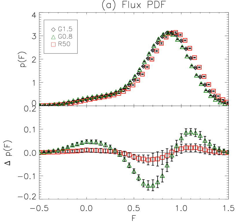
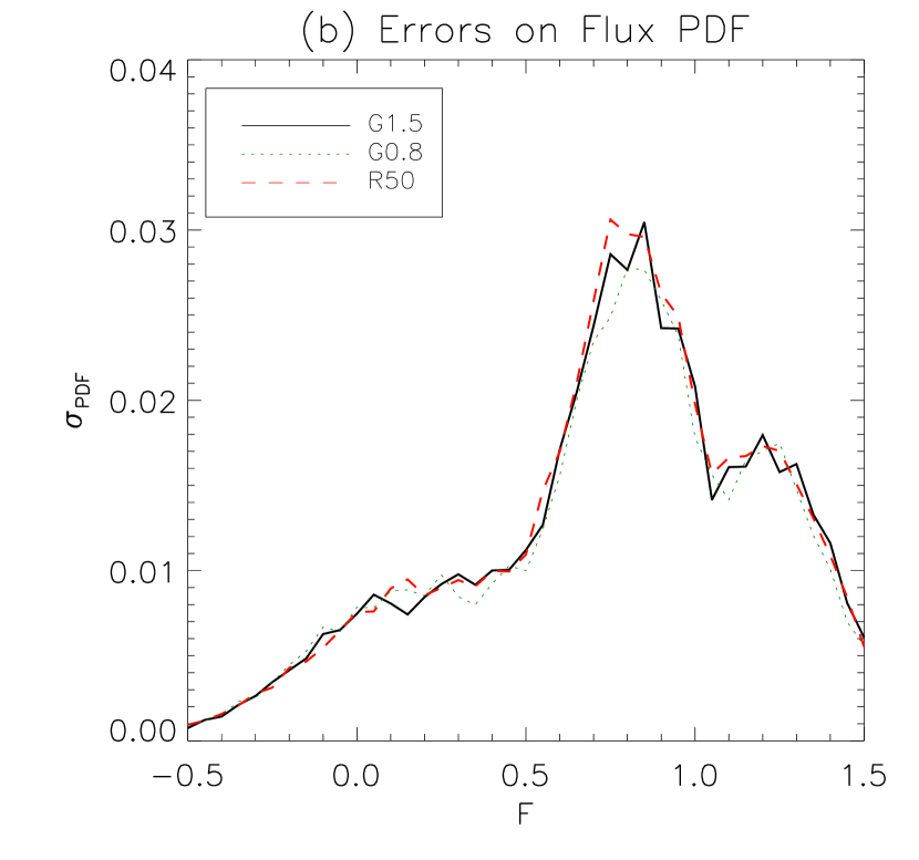
Figure 4.— (a) Top panel shows the flux PDF from 600 mock spectra with $\mathrm{S/N}=4$ per pixel at $z=2.5$, generated for models G1.5 (black diamonds), G0.8 (green triangles), and R50 (red squares). The points are offset horizontally for clarity. Lower panel shows the difference in the PDF between models G0.8 and G1.5 (green triangles), and between models R50 and G1.5 (red squares). (b) Estimated errors on the flux PDF from models G1.5 (black solid line), G0.8 (green dotted line), and R50 (red dashed line). See electronic edition of the Journal for a color version of this figure.

In order to provide a comparison for our assumed systematics vis-á-vis Desjacques et al. (2007), we evaluate the PDF for our toy models computed from mock samples similar to the DR3 data, i.e. 600 spectra with $\mathrm{S/N}=4$ per pixel at $z\sim 2.5$.

The resultant PDFs for models G1.5, G0.8, and R50, are shown in the top panel of Figure 4a, with each PDF divided into bins of width $\Delta F=0.05$. The error bars are the $1\;\sigma$ dispersion from $\sim 100$ realizations. These realizations have different random seeds for the instrumental noise, and cosmic variance is included by drawing each realization from different lines-of-sight in the simulation box and generating the bubble distributions separately in the case of the inhomogeneous models. The errors are plotted explicitly in Figure 4b.

The PDFs from our mock spectra have the general characteristics expected from noisy Ly$\alpha$ forest spectra, e.g. the existence of pixels with $F<0$ and $F>1$. The fact that the plots in Figure 4a are clearly different from the PDFs of high-resolution spectra e.g. in Kim et al. (2007) underlines the fact that the flux PDF is sensitive to noise and other systematics. We do not expect our PDF to match the observed SDSS PDFs in Desjacques et al. (2007) exactly as our mock spectra are generated from simulations that do not have the right small-scale power, nor did we carry out a detailed consideration of the systematics such as instrumental noise. Such a careful approach would be required when analyzing real data in order to constrain a priori the overall Ly$\alpha$ forest parameters, but in this paper we are concerned with the differences arising from the IGM with respect to a fiducial model, so the fiducial model itself does not need to be exactly right for our tests.

We use the errors on the PDFs as a check on our assumptions regarding the systematics. As expected, increasing the scatter $\sigma_{F}$ of the continuum levels increases the error bars on the PDF. We find that the errors from our mock PDFs, Figure 4b, and those of Desjacques et al. (2007) (Figure 7 in their paper) are similar when we use $\sigma_{F}=9\%$ as suggested by Suzuki et al. (2005). This indicates that our simplified models for the SDSS instrumental effects and sample properties provide a reasonable estimate for the sample errors. For our DR7 mock samples in the later parts of this paper we will henceforth assume that the shape of the quasar continuum can be fit perfectly, and set errors in the continuum level to $\sigma_{F}=9\%$.

The lower panel of Figure 4a shows the differences in PDF with respect to the fiducial model G1.5, $\Delta p(F)_{\mathrm{model}}=p(F)_{\mathrm{model}}-p(F)_{G1.5}$. Interestingly, it is clear that even with the DR3 data set it would have been possible to distinguish an inverted equation of state, G0.8, from the fiducial model G1.5 at high significance.

In order to quantify the ability of the PDF to distinguish between the different models, we compute a logarithmic likelihood

$$-\ln\mathcal{L}(\mu_{i}|x_{i})=\frac{1}{2}(x_{i}-\mu_{i})^{T}C_{ij}^{-1}(x_{j}-\mu_{j}),$$ (9)

where we assume the PDF for one model, $x_{i}$ – the subscript refers to the bins in the data –, to be the ‘observed’ data and take the mean PDF for another model $\mu_{i}$ as the ‘theory’ points, and $C_{ij}$ is the covariance matrix for $x_{i}$ (in this case directly evaluated from the mock realizations). A small value of $-\ln\mathcal{L}\sim 1$ indicates that the ‘theory’ model is consistent with the ‘observed’ model and hence the two models cannot be differentiated. As the estimated errors are similar for all the models as shown in Figure 4b, in practice $x_{i}$ and $\mu_{i}$ are interchangeable for any two models. When evaluating Equation 9 on the flux PDF we use only bins in the range $0.4\leq F\leq 1.1$, which excludes the lower and upper 10% of the flux distribution.

Table 1 summarizes the results from assuming a DR7 sample size (1500 quasars) and the systematics we have assumed. Each entry in the table shows $-\ln\mathcal{L}$ for distinguishing between PDF of the ‘observed’ model in the corresponding column, and the PDF of ‘theory’ model in the corresponding row.

Table 1 $-\ln\mathcal{L}$ between PDFs for different IGM models

	G1.5	G1.3	G0.8	R50	R25	I50
G1.5	0.0	21.8	388.5	15.4	11.1	18.1
G1.3	$\cdots$	0.0	154.1	2.3	2.2	2.3
G0.8	$\cdots$	$\cdots$	0.0	209.1	159.8	218.7
R50	$\cdots$	$\cdots$	$\cdots$	0.0	0.2	0.2
R25	$\cdots$	$\cdots$	$\cdots$	$\cdots$	0.0	0.1
I50	$\cdots$	$\cdots$	$\cdots$	$\cdots$	$\cdots$	0.0

Note. — Assumes mock SDSS DR7 data set of 1500 quasars at $z=2.5$, with $\mathrm{S/N}=4$ in the Ly$\alpha$ forest.

We find that the PDF can distinguish G0.8 from G1.5 with a high significance of $-\ln\mathcal{L}({\mathrm{G}0.8|G1.5})=388.5$. At first glance, we get the surprising result that the PDF can differentiate the inhomogeneous He II reionization model R50 from the fiducial G1.5 at a significant $-\ln\mathcal{L}({\mathrm{R}50|G1.5})=15.4$. However, note that the models R50 and G1.3 are approximately degenerate with $-\ln\mathcal{L}({\mathrm{R}50|G1.3})=2.3$ between the two models. This is because the PDF of R50 is essentially averaged across its two different phases of $\gamma=1.2$ and $\gamma=1.5$, thus it can be fit by a homogeneous model with some intermediate value of $\gamma$.

As expected, we find that the PDF is degenerate between the models R50, R25, and I50 since the only difference is the spatial distribution of the line-of-sight segments which intersect with hot bubbles.

There are several uncertainties in the IGM parameters which might be degenerate with $\gamma$ in the flux PDF. The Jean’s smoothing scale of the IGM is dependent on physics such as complex hydrodynamic effects and the temperature evolution of the gas, which are not very well understood. Gnedin & Hui (1998b) have argued for an effective smoothing scale which is approximately half the Jean’s scale at the epoch of observation. This gives $\sigma_{eff}\approx 0.15\,h^{-1}\,\mathrm{Mpc}$ at $z=2$. As the Slosar et al. (2009) simulations used in this paper do not accurately capture small-scale power ($\sigma_{eff}=0.25\,h^{-1}\,\mathrm{Mpc}$ was used), we turn to another set of simulations: the White et al. (2010) ‘Roadrunner’ simulations are similar to those of Slosar et al. (2009) except with higher resolution ($0.1875\,h^{-1}\,\mathrm{Mpc}$ grid size vs $0.5\,h^{-1}\,\mathrm{Mpc}$) and smaller box ($(750\,h^{-1}\,\mathrm{Mpc})^{3}$ vs $(1500\,h^{-1}\,\mathrm{Mpc})^{3}$). The smoothing scale used in the Roadrunner simulations is $\sigma_{eff}=0.1\,h^{-1}\,\mathrm{Mpc}$. To approximate the uncertain pressure smoothing scale on the flux PDF, we take the optical depth outputs of these simulations and smooth them to an overall smoothing scale of $\sigma_{eff}=0.15\,h^{-1}\,\mathrm{Mpc}$ using a Gaussian kernel. In comparison with the original spectra, we find that the resulting flux PDFs differ by only $-\ln\mathcal{L}(\sigma_{eff}=0.15\,h^{-1}\,\mathrm{Mpc}|\sigma_{eff}=0.1\,h^{-1}\,\mathrm{Mpc})\approx 2$, which is significantly less than the difference caused by varying $\gamma$. In any case, in the future data analysis we expect to use hydrodynamic simulations which would obviate the need to explicitly assume a value for the Jean’s smoothing scale.

Another systematic which could be degenerate with $\gamma$ are the uncertainties in the value of the mean flux of the Ly$\alpha$ forest $\langle F\rangle$, which we have thus far assumed to be fixed. Using the somewhat smaller SDSS Data Release 5, Dall’Aglio et al. (2009) reported errors in their measurements of $\tau_{eff}\equiv-\ln\langle F\rangle$ equivalent to $\sigma_{F}\approx 0.3\%$ in the mean flux at $z\approx 2.5$. We study the effect of this uncertainty by assuming the actual mean flux is distributed as a Gaussian distribution with $\sigma_{F}=0.3\%$, and marginalizing over this when calculating the likelihoods between the different values of $\gamma$. This gives a value of $-\ln\mathcal{L}(G1.3|G1.5)\approx 15$ in comparison with $-\ln\mathcal{L}(G1.3|G1.5,\delta\langle F\rangle=0)\approx 20$ reported in Table 1 This is a significant effect and needs to be taken into account in a more formal data analysis, but does not qualitatively affect our conclusions.

In general, we have found that the flux PDF from the latest SDSS data can be used to constrain the equation of state of the IGM if a homogeneous IGM is assumed. Indeed, the evolution of $\gamma$ with redshift can potentially be measured. In the SDSS DR7 quasar catalog there are more than 700 quasars with $\mathrm{S/N}\geq 4$ in the Ly$\alpha$ forest within redshift bins of $\Delta z=0.3$ up to $z_{qso}\sim 3.5$. The logarithmic likelihood $-\ln\mathcal{L}$ is roughly proportional to sample size, thus in comparison with our mock sample size of 1500 quasars at $2.4\leq z_{qso}\leq 2.7$ and the results of Table 1, we expect to be able to measure the IGM equation of state in these redshift bins to a precision of $\Delta\gamma\sim 0.2$ with a confidence of $-\ln\mathcal{L}\sim 10$ (approximately $4\sigma$), although it becomes more difficult to estimate accurately the quasar continuum in the Ly$\alpha$ forest at higher redshifts.

These simulations suggest that an analysis on the flux PDF from the SDSS sample could detect the predicted suppression in the equation of state from $\gamma\approx 1.5$ to $\gamma\lesssim 1$ (see Furlanetto & Oh 2008b; McQuinn et al. 2009) due to He II reionization at $z\sim 3$. Note that this approach is complementary to studies which used the evolution of the mean optical depth $\tau_{\mathrm{eff}}$ in the Ly$\alpha$ forest to study He II reionization, since the PDF can in principle be used to measure $\gamma$ at fixed $\langle F\rangle=\exp({-\tau_{\mathrm{eff}}})$.

5. Threshold Probability Functions from Mock Spectra

In this section, we evaluate the threshold correlation statistics $S_{2}$, $C_{2}$, and $D_{2}$ on the mock Ly$\alpha$ forest sample described in the previous sections. We first describe the form of these functions, before applying them to the various IGM models and investigate their ability to distinguish between models.

5.1. Basic Form of $S_{2}$, $C_{2}$, and $D_{2}$ on the Ly$\alpha$ Forest

As we are primarily interested in breaking the degeneracy between the equation of state of the IGM and thermal inhomogeneities with comoving scales of $\sim 10\,h^{-1}\,\mathrm{Mpc}$, we first smooth the mock Ly$\alpha$ forest spectra with a Gaussian window of width $\sigma=10\,h^{-1}\,\mathrm{Mpc}$. This has the effect of increasing the contrast from the temperature inhomogeneities and smoothing over the noise, although after smoothing the shapes of the spectra are still dominated by instrumental noise and the large-scale structure of matter. In other words, when visually inspecting the smoothed spectra of the same line-of-sight modified to the different IGM models, it is still impossible to tell a priori which is the inhomogeneous model.

For each value of $F_{th}$, we first identify the pixels which have $F\geq F_{th}$ within each individual smoothed spectrum, keeping track of the ‘clusters’ of adjoined pixels. $S_{2}(r,F_{th})$ is then calculated by counting pairs of pixels above $F_{th}$, and separated by correlation length $r$. This is then normalized to give a probability. We also keep track of $C_{2}(r,F_{th})$ as the probability of pixel pairs which are within the same cluster of pixels with $F\geq F_{th}$. The threshold probability functions are then evaluated on a 2-dimensional grid in $F_{th}$ and $r$ on the SDSS DR7 mock samples.

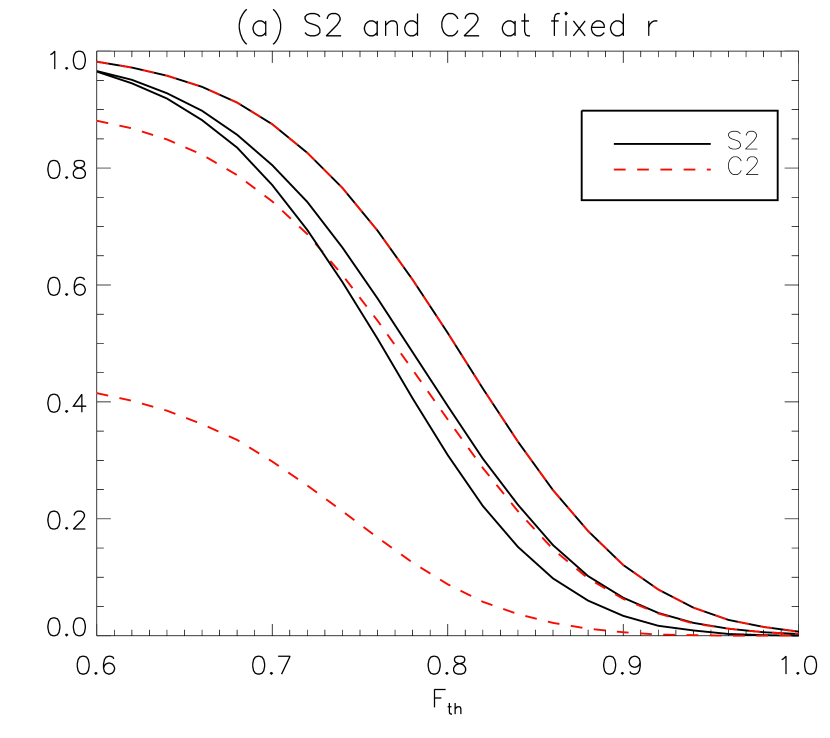
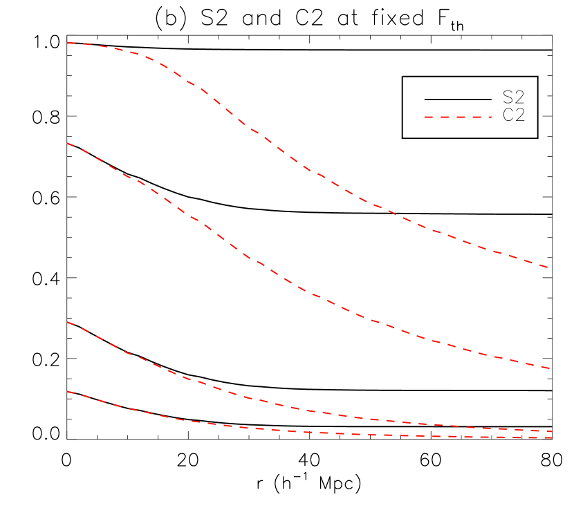
Figure 5.— (a) $S_{2}$ (solid black lines) and $C_{2}$ (dashed red lines) from model G1.5 plotted as a function of flux threshold $F_{th}$ at fixed comoving distances (from top to bottom) $r=0\,h^{-1}\,\mathrm{Mpc},15\,h^{-1}\,\mathrm{Mpc},60\,h^{-1}\,\mathrm{Mpc}$. Note that $S_{2}$ and $C_{2}$ overlap in the case of $r=0\,h^{-1}\,\mathrm{Mpc}$ (uppermost plot). (b) $S_{2}$ and $C_{2}$ plotted as a function of comoving distance $r$ at fixed flux threshold $F_{th}=0.6,0.75,0.85,0.9$ from top to bottom. See electronic edition of the Journal for a color version of this figure.

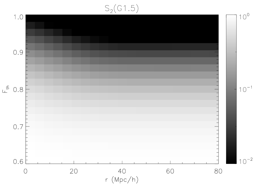
Figure 6.— 2-dimensional density plot of $S_{2}$ as a function of $F$ and $r$, evaluated for one mock sample based on the model G1.5.

Figure 5a plots $S_{2}(F_{th})$ and $C_{2}(F_{th})$ at fixed $r$ for the fiducial model G1.5 (recall that $S_{2}=C_{2}+D_{2}$, Equation 5). At large $F_{th}$ few pixels in the smoothed spectra have sufficiently large flux $F$ to rise above the threshold, thus $S_{2}(F_{th}|r)$ tends to zero at all $r$ as $F_{th}\rightarrow 1$. Conversely, as the threshold is lowered below the mean flux $\langle F\rangle$, increasing numbers of pixels satisfy the criterion $F\geq F_{th}$ and $S_{2}$ trends towards unity,

$$\lim_{F_{th}<\overline{F}}S_{2}(F_{th}|r)=1.$$ (10)

At small pixel separations $r$, the main contribution to $S_{2}$ comes from $C_{2}$ as most pixel pairings that rise above the flux threshold are within the same cluster of pixels (recall that ‘clusters’ in this context refers to groupings of contiguous pixels and not galaxy or stellar clusters). Note that $S_{2}(F_{th}|r=0)\equiv C_{2}(F_{th}|r=0)$ is just the integral of the flux PDF (see Equation 6). The contribution of $C_{2}$ to $S_{2}$ decreases and gives way to $D_{2}\equiv S_{2}-C_{2}$ at greater $r$ as there is greater probability of finding pixels from different clusters than within the same cluster.

Figure 5b plots $S_{2}$ and $C_{2}$ as a function of $r$ at fixed values of $F_{th}$. This shows more clearly the trend of $C_{2}$ dominating the probability of pixels pairs being above the flux threshold at small separations. The overall probability $S_{2}$ increases as the flux threshold is lowered and more pixels satisfy the condition $F\geq F_{th}$. At separations larger than $r\gtrsim 50\,h^{-1}\,\mathrm{Mpc}$, $D_{2}$ dominates and we see the asymptotic behaviour $S_{2}(r|F_{th})\rightarrow S_{2}^{2}(0|F_{th})$ as the pixel separations at large scales is effectively random. As $S_{2}(r=0|F_{th})$ and its square essentially measure the integral of the flux PDF (Equation 6), we expect any additional information from $S_{2}$ to come at small correlation lengths $r\lesssim 50$, i.e. from $C_{2}$.

Figure 6 displays $S_{2}$ as a density plot in the two dimensions of $r$ and $F_{th}$.

5.2. Distinguishing Between IGM Models

We compute $S_{2}$ on realizations of DR7 mock samples computed for the various IGM models introduced in Section 3, using the systematics and mock sample previously discussed (1500 lines-of-sight with $\mathrm{S/N}$=4, flux errors $\sigma_{F}=9\%$). The mock data are evaluated on 2-dimensional grids in the ranges $0\,h^{-1}\,\mathrm{Mpc}\geq r\geq 80\,h^{-1}\,\mathrm{Mpc}$ and $0.5\geq F_{th}\geq 1.0$, with 26 bins in each dimension.

As was done for the PDFs in Section 4.2, we use the logarithmic likelihood $-\ln\mathcal{L}$  (Equation 9) to quantify the ability to differentiate the different IGM models. From the initial 676 data points for $S_{2}(r,F_{th})$ from each model, we first remove $\sim 20$ points with $S_{2}<10^{-3}$ to reduce the dynamic range, and then remove a few more points in order to ensure that the covariance matrix (calculated from $\sim 100$ mock realizations for each model) is well-conditioned.

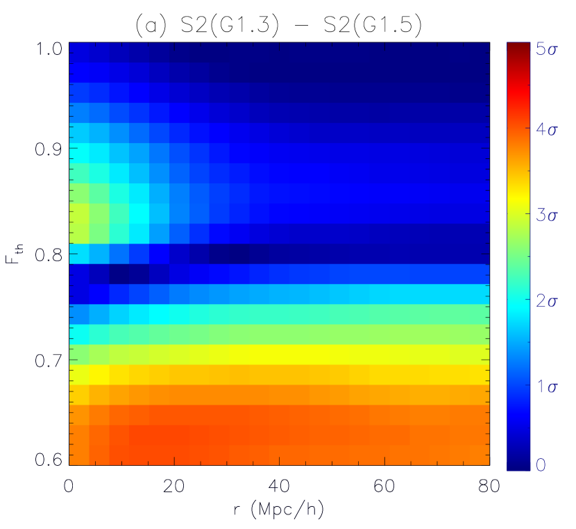
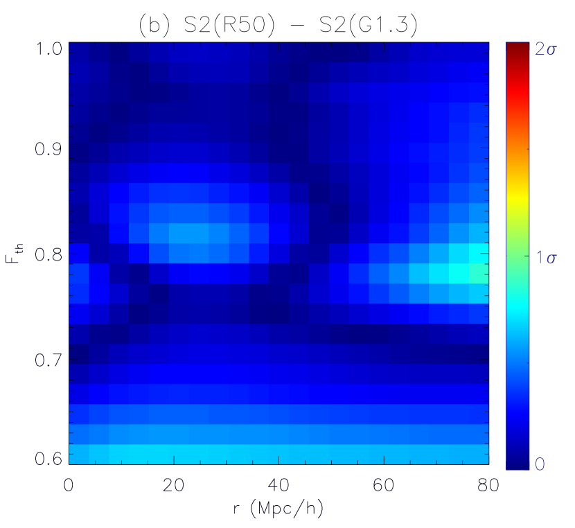
Figure 7.— (a) Absolute difference between $S_{2}$ from models G1.3 and G1.5 as a function of $r$ and $F_{th}$, normalized by the error from the former. (b) Absolute difference between $S_{2}$ from models R50 and G1.3. Note different intensity scale from plot on the left. See electronic edition of the Journal for a color version of this figure.

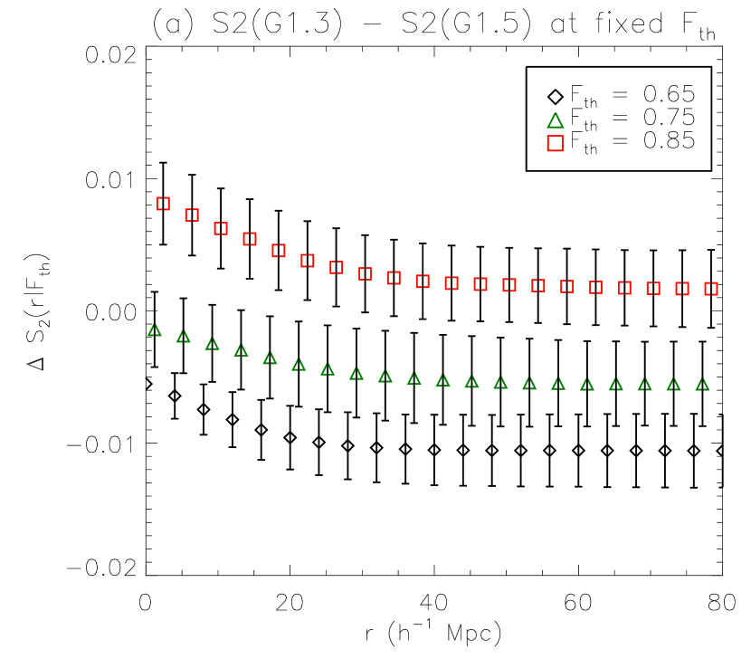
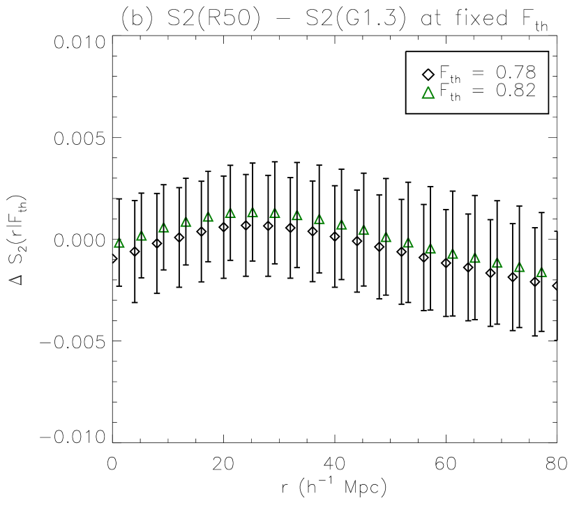
Figure 8.— (a) Difference between $S_{2}$ from models G1.3 and G1.5, plotted as a function of correlation length $r$ at fixed values of $F_{th}=0.65$ (black diamonds), $F_{th}=0.75$ (green triangles), and $F_{th}=0.85$ (blue squares). The points are offset horizontally for clarity. (b) Difference between $S_{2}$ from models R50 and G1.3, as a function of $r$ at fixed values of $F_{th}=0.78$ (black diamonds) and $F_{th}=0.82$ (green triangles). The different shape of (b) compared to (a) indicates the biasing of $S_{2}$ towards larger $r$ due to the presence of temperature inhomogeneities in R50. See electronic edition of the Journal for a color version of this figure.

The values of $-\ln\mathcal{L}$  between the various models are summarized in Table 2. In general, we see that the threshold probability function does a somewhat better job of distinguishing between the homogeneous models: $-\ln\mathcal{L}(G1.3|G1.5)=54.1$ between models G1.5 and G1.3 compared with $-\ln\mathcal{L}(G1.3|G1.5)=21.8$ when using the PDF computed for the same mock samples (Table 1).

The absolute differences $\Delta S_{2}$ between the two models as a function of $r$ and $F_{th}$ are shown in Figure 7a, normalized by the estimated error in each point. Figure 8a plots the difference between these two models as a function of $r$ at several fixed values of $F_{th}$. It can be seen that the plots of $\Delta S_{2}(r|F_{th})$ have the same general shape as $S_{2}(r|F_{th})$ (Figure 5b) at the various values of $F_{th}$ shown, which shows that $\Delta S_{2}$ between these two models includes contributions from all comoving scales.

Table 2 $-\ln\mathcal{L}$ between $S_{2}(r,F_{th})$ for different IGM models, assuming 9% flux continuum error

	G1.5	G1.3	G0.8	R50	R25	I50
G1.5	0.0	54.1	837.6	67.8	65.3	69.1
G1.3	$\cdots$	0.0	400.6	14.1	7.2	17.7
G0.8	$\cdots$	$\cdots$	0.0	439.1	433.3	389.2
R50	$\cdots$	$\cdots$	$\cdots$	0.0	4.5	3.2
R25	$\cdots$	$\cdots$	$\cdots$	$\cdots$	0.0	4.1
I50	$\cdots$	$\cdots$	$\cdots$	$\cdots$	$\cdots$	0.0

Note. — Assumes mock SDSS DR7 data set of 1500 quasars at $z=2.5$, with $\mathrm{S/N}=4$ in the Ly$\alpha$ forest.

However, $S_{2}$ has some ability to break the degeneracy between the models G1.3 and R50 with $-\ln\mathcal{L}(R50|G1.3)=14.1$, compared with $-\ln\mathcal{L}(R50|G1.3)=2.3$ using the PDF. Figure 7b shows $|\Delta S_{2}(r,F_{th})|$ for models R50 and G1.3, and we see that the differences are relatively subtle with $|\Delta S_{2}(r,F_{th})|\lesssim 1\sigma$. In Figure 8b, the plots of $\Delta S_{2}(r|F_{th})$ shows that the deviations do not trace the shape of $S_{2}(r|F_{th})$, but have a hump-like shape peaking at scales of $r\sim 20\,h^{-1}\,\mathrm{Mpc}$ and extending well into the larger scales where $S_{2}(r|F_{th})$ goes flat in Figure 5b . A comparison with Figure 5b suggests that most of this contribution comes from $C_{2}$. However, if the bubbles have a smaller characteristic size then they are harder to distinguish from the closest homogeneous model: $-\ln\mathcal{L}(R25|G1.3)=7.2$ which would be a marginal detection.

As we have discussed, the temperature inhomogeneities in the IGM are too subtle to overcome the density field which dominates the optical depth distribution of the IGM, but regions of higher temperature such as those shown in Figure 3 can broaden the width of pixel clusters that rise above the flux threshold $F_{th}$ when averaged across many spectra, increasing $S_{2}$ at the scales represented by the various path lengths at which the Ly$\alpha$ lines-of-sight intersect the hot bubbles. The shape of $\Delta S_{2}$ in Figure 5b represents a slight broadening of $C_{2}$ from the hot bubbles in the model. While a homogeneous IGM with $\gamma\approx 1.3$ can provide a flux PDF that is indistinguishable from an inhomogeneous model, the threshold correlation functions measures sufficient spatial information to detect the temperature inhomogeneities and break the degeneracy with the best-fit homogeneous model.

In addition, we see from Table 2 that the model R25 with smaller hot bubbles is difficult to distinguish from model R50 with $-\ln\mathcal{L}(R25|R50)=4.5$, but the fact that $-\ln\mathcal{L}$  is not of order unity indicates that $S_{2}$ encodes some information on the characteristic scale of the temperature inhomogeneities. Looking at the inverted bubble model I50, we see that it is nearly degenerate with R50, with $-\ln\mathcal{L}=3.2$ between the two models. Nevertheless, it would appear that all the inhomogeneous models can be differentiated from G1.3 with $-\ln\mathcal{L}\gtrsim 10$ in comparison with $-\ln\mathcal{L}\sim 1$ when using the PDF.

5.3. Improved Flux Continuum Estimates

In our mock spectra we have so far assumed what we regard as a worst-case scenario for estimating the flux continuum of the Ly$\alpha$ forest, with errors of around 9%. This was the uncertainty that Suzuki et al. (2005) found from PCA fitting on the intrinsic quasar spectrum redwards of the Ly$\alpha$ emission line and without using any information from the Ly$\alpha$ forest itself.

There are various possibilities to improve on the flux continuum fits. One method is to assume that the mean flux $\overline{F}$ for each Ly$\alpha$ forest is equal to the global mean flux $\langle F(z)\rangle$ at the corresponding redshift, and normalize the observed quasar continuum to this value (N. Suzuki, private communication). In this way, the errors in the continuum fit would be limited to a combination of cosmic variance and errors in the determination of the mean flux. The dispersion in the mean flux between different lines-of-sight is of order 1-2%, while within an individual line-of-sight with e.g. $\mathrm{S/N}\sim 4$ across $\sim 500$ pixels the mean flux can be determined to about $(S/N\times\sqrt{(}500))^{-1}\sim 1\%$. In principle, this yields an error on the continuum determination at the few percent level (N. Suzuki, private communication).

In this subsection, we compute the threshold probability functions for mock spectra with assumed flux continuum errors of $\sigma_{F}=3\%$, which is an optimistic estimate of the precision believed possible with the mean flux fitting method. In all other respects, the properties of our mock sample are unchanged from the previous sections.

Table 3 $-\ln\mathcal{L}$ between $S_{2}(r,F_{th})$ for different IGM models, assuming 3% flux continuum error

	G1.5	G1.3	G0.8	R50	R25	I50
G1.5	0.0	150.1	1620.7	205.3	181.0	191.1
G1.3	$\cdots$	0.0	779.6	29.0	21.9	28.6
G0.8	$\cdots$	$\cdots$	0.0	756.8	707.2	965.9
R50	$\cdots$	$\cdots$	$\cdots$	0.0	15.1	2.7
R25	$\cdots$	$\cdots$	$\cdots$	$\cdots$	0.0	10.4
I50	$\cdots$	$\cdots$	$\cdots$	$\cdots$	$\cdots$	0.0

Note. — Assumes mock SDSS DR7 data set of 1500 quasars at $z=2.5$, with $\mathrm{S/N}=4$ in the Ly$\alpha$ forest.

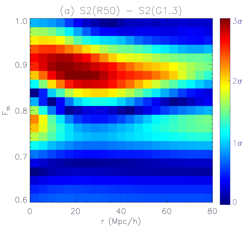
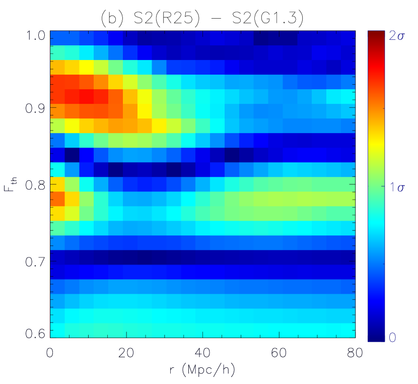
Figure 9.— (a) Absolute difference between $S_{2}$ from models R50 and G1.3 as a function of $r$ and $F_{th}$, normalized by the error from the former. These were calculated assuming 3% errors in the continuum determination. (b) Absolute difference between $S_{2}$ from models R25 and G1.3, assuming 3% continuum errors. Note that the differences in (b) peak at smaller scales.

Table 3 summarizes the logarithmic likelihoods for differentiating $S_{2}$ calculated from any two IGM models. Overall, the values of $-\ln\mathcal{L}$ see a marked improvement when compared with the values in Table 2 computed assuming 9% flux continuum errors. It is now possible to tell the inhomogeneous models apart from the model G1.3 with significant confidence, with $-\ln\mathcal{L}\gtrsim 30$.

More importantly, $S_{2}$ can now place significant constraints on the characteristic scale of the He II reionization bubbles, as $-\ln\mathcal{L}(R25|R50)=15.1$. The differences can be clearly seen in the two-dimensional differences plots of $S_{2}(r,F_{th})$ of these models with respect to that calculated from the best-fit homogeneous model G1.3, Figure 9. The deviations from the model G1.3 peak at smaller scales $r$ in the case of R25, Figure 9b, compare R50, Figure 9a. This effect can be seen more emphatically in Figure 10, which shows $\Delta S_{2}$ between R25 and R50 plotted at several flux threshold values. At the flux threshold values shown, R50 displays a distinct increase in $S_{2}$ at larger scales compared with R25.

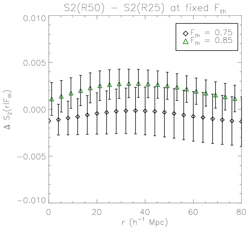
Figure 10.— Difference between $S_{2}$ from models R50 and R25, plotted as a function of correlation length $r$ at fixed values of $F_{th}=0.75$ (black diamonds) and $F_{th}=0.85$ (green triangles). The points are offset horizontally for clarity. See electronic edition of the Journal for a color version of this figure.

Even with the improved precision for the flux continuum, $S_{2}$ is still unable to distinguish between R50 and its topologically inverted counterpart I50, with $-\ln\mathcal{L}=2.7$ for differentiating the two models. This is not surprising, as Figure 2 shows that the size distribution of hot and cold regions in the R50 and I50 boxes are similar due to the equal volume fractions.

6. Discussion & Conclusion

In this paper we have introduced to astrophysics a set of new correlation statistics, $S_{2}$, $C_{2}$, and $D_{2}$, that are evaluated as two-dimensional functions of correlation length $r$ and transmitted flux threshold $F_{th}$. These ‘threshold probability functions’ were tested on mock Ly$\alpha$ forest spectra in which instrumental noise and systematics were added at a level appropriate to the SDSS Ly$\alpha$ forest data, and we have made assumptions on the flux continuum errors based on the PCA fitting method of Suzuki et al. (2005).

6.1. Flux PDF

As the threshold correlation statistics can be thought of as the flux probability distribution function (PDF) measured as a function of spatial scale, we first computed the flux PDF in order to check that the errors from our mock spectra are comparable with those of the observed PDF from SDSS spectra published in Desjacques et al. (2007). At the level of uncertainty arising from the latest SDSS data set, we find that with the assumption of a homogeneous IGM the flux PDF can in fact constrain the IGM equation of state, $\gamma$, to $\Delta\gamma\sim 0.1$ at the $\sim 4\sigma$ level in redshift bins of $\Delta z\sim 0.3$. This would allow the redshift evolution of $\gamma$ to be constrained through the epoch of He II reionization at $z\approx 3$.

To-date, the best constraints on the equation of state $\gamma$ of the IGM have come from flux PDFs measured from small numbers ($\sim 20$) of high-resolution Ly$\alpha$ forest spectra, which have favored an inverted equation of state $\gamma<0$ (Becker et al. 2007; Kim et al. 2007; Viel et al. 2009). In a subsequent paper we aim to measure the flux PDF from SDSS DR7, and in conjunction with numerical simulations and detailed modelling of systematics make independent measurements of $\gamma$ as a function of redshift. This would be an interesting complement to the studies using the mean flux evolution in the Ly$\alpha$ forest, which have placed the completion of He II reionization at $z\approx 3.2$ (Bernardi et al. 2003).

Baryon Oscillation Spectroscopic Survey (BOSS), part of the third phase of the SDSS (SDSS-III), aims to observe $\sim$ 150,000 quasar lines-of-sight. While many of these Ly$\alpha$ forest spectra will be of low signal-to-noise ($\mathrm{S/N}\sim 1$), there will be sufficient numbers of moderate $\mathrm{S/N}$ spectra that even better constraints can be made on the He II end-of-reionization epoch than the DR7 sample considered in this paper.

6.2. Threshold Probability Functions

We have tested the threshold probability functions on the mock spectra, and found that they are able to break the degeneracy between an IGM with temperature inhomogeneities and the best-fit homogeneous model of $\gamma=1.3$, at a confidence of $\sim 5\sigma$.

If the errors in the continuum fitting can be reduced to $\sigma_{F}\approx 3\%$, then $S_{2}$ is sensitive to the characteristic scale of the temperature inhomogeneities, being able to distinguish between toy models with 50$\,h^{-1}\,\mathrm{Mpc}$ and 25$\,h^{-1}\,\mathrm{Mpc}$ bubbles at $\sim 5\sigma$.

In this paper we have taken a simplified approach towards the instrumental systematics and noise in the mock spectra. This has provided adequate estimates for our errors, but would be insufficient to constrain the IGM from real data. Some of the systematics we have not taken into account include the possible influence of damped Ly$\alpha$ (DLA) regions in the Ly$\alpha$ forest, metal line absorption, etc. All these need to be modelled in detail when analyzing real data. As for the flux continuum fitting, we hope to use methods such as mean-flux fitting to reduce the errors to several percent, which would enable the threshold probability functions to constrain the physical scale of any thermal inhomogeneities in addition to making a detection. Whatever the method used, the residual errors that arise need to be well-characterized in order to be modelled in the data analysis.

The mock spectra used in this paper have been generated using dark matter-only simulations that do not capture detailed IGM physics, and various toy models for the IGM have been ‘painted’ on to the basic set of mock spectra. In the actual data analysis we anticipate fitting the data to mock spectra based on more detailed numerical simulations that include the physics of He II reionization. This would allow, in addition to a direct measurement of the temperature range $\Delta T$ and spatial scale of the inhomogeneities, constraints to be placed on the underlying physical mechanisms such as the quasar luminosity function and duty cycle, background ionization rate, gas clumping factors etc.

In the near future, the high area density of the BOSS quasars will enable correlation studies in the transverse direction between quasar pairs. It would be straightforward to extend the threshold probability functions to work in both the parallel and transverse directions relative to line-of-sight in order to utilize the full power of the BOSS data. In addition, transverse studies would ameliorate the effects of the uncertain fitting of the quasar continuum. However, we defer the three-dimensional generalization of the threshold probability functions to a future paper.

6.3. Summary

Using mock Ly$\alpha$ forest spectra based on toy models of the IGM and simulations of the existing SDSS data, we have shown that detailed statistical analysis of these spectra can provide insight into the physics of the IGM:

• The flux PDF from the SDSS DR7 can place significant constraints on the equation of state $\gamma$ of a homogeneous IGM to $\Delta\gamma\sim 0.1$ at $z\approx 2.5$, and track its evolution through the end of He II reionization.
  

• We have introduced the threshold probability functions $S_{2}$, $C_{2}$, and $D_{2}$, which measure the Ly$\alpha$ forest as functions of flux level and spatial scale, and have shown that they can differentiate an inhomogeneous IGM from the best-fit homogeneous model at $\gtrsim 3\sigma$.
  

• If the flux continuum fitting can be carried out to $\approx 3\%$ accuracy, the threshold statistics can place constraints on the characteristic scale of the temperature inhomogeneities.

References

- Becker et al. (2007) Becker, G. D., Rauch, M., & Sargent, W. L. W. 2007, ApJ, 662, 72
- Bernardi et al. (2003) Bernardi, M., Sheth, R. K., SubbaRao, M., Richards, G. T., Burles, S., Connolly, A. J., Frieman, J., Nichol, R., et al. 2003, AJ, 125, 32
- Cen et al. (1994) Cen, R., Miralda-Escudé, J., Ostriker, J. P., & Rauch, M. 1994, ApJ, 437, L9
- Croft et al. (2002) Croft, R. A. C., Weinberg, D. H., Bolte, M., Burles, S., Hernquist, L., Katz, N., Kirkman, D., & Tytler, D. 2002, ApJ, 581, 20
- Croft et al. (1998) Croft, R. A. C., Weinberg, D. H., Katz, N., & Hernquist, L. 1998, ApJ, 495, 44
- Dall’Aglio et al. (2009) Dall’Aglio, A., Wisotzki, L., & Worseck, G. 2009, ArXiv e-prints
- Davé et al. (1999) Davé, R., Hernquist, L., Katz, N., & Weinberg, D. H. 1999, ApJ, 511, 521
- Desjacques et al. (2007) Desjacques, V., Nusser, A., & Sheth, R. K. 2007, MNRAS, 374, 206
- Fan et al. (2002) Fan, X., Narayanan, V. K., Strauss, M. A., White, R. L., Becker, R. H., Pentericci, L., & Rix, H. 2002, AJ, 123, 1247
- Faucher-Giguère et al. (2008) Faucher-Giguère, C., Prochaska, J. X., Lidz, A., Hernquist, L., & Zaldarriaga, M. 2008, ApJ, 681, 831
- Furlanetto & Oh (2008a) Furlanetto, S. R. & Oh, S. P. 2008a, ApJ, 682, 14
- Furlanetto & Oh (2008b) —. 2008b, ApJ, 681, 1
- Gnedin & Hui (1998a) Gnedin, N. Y. & Hui, L. 1998a, MNRAS, 296, 44
- Gnedin & Hui (1998b) —. 1998b, MNRAS, 296, 44
- Hui & Gnedin (1997) Hui, L. & Gnedin, N. Y. 1997, MNRAS, 292, 27
- Jenkins & Ostriker (1991) Jenkins, E. B. & Ostriker, J. P. 1991, ApJ, 376, 33
- Jiao et al. (2009) Jiao, Y., Stillinger, F. H., & Torquato, S. 2009, Proceedings of the National Academy of Sciences, 106, 17634
- Kim et al. (2007) Kim, T., Bolton, J. S., Viel, M., Haehnelt, M. G., & Carswell, R. F. 2007, MNRAS, 382, 1657
- Lai et al. (2006) Lai, K., Lidz, A., Hernquist, L., & Zaldarriaga, M. 2006, ApJ, 644, 61
- Lidz et al. (2009) Lidz, A., Faucher-Giguere, C., Dall’Aglio, A., McQuinn, M., Fechner, C., Zaldarriaga, M., Hernquist, L., & Dutta, S. 2009, ArXiv e-prints
- Lidz et al. (2006) Lidz, A., Heitmann, K., Hui, L., Habib, S., Rauch, M., & Sargent, W. L. W. 2006, ApJ, 638, 27
- McDonald et al. (2001) McDonald, P., Miralda-Escudé, J., Rauch, M., Sargent, W. L. W., Barlow, T. A., & Cen, R. 2001, ApJ, 562, 52
- McDonald et al. (2000) McDonald, P., Miralda-Escudé, J., Rauch, M., Sargent, W. L. W., Barlow, T. A., Cen, R., & Ostriker, J. P. 2000, ApJ, 543, 1
- McDonald et al. (2006) McDonald, P., Seljak, U., Burles, S., Schlegel, D. J., Weinberg, D. H., Cen, R., Shih, D., Schaye, J., et al. 2006, ApJS, 163, 80
- McDonald et al. (2005) McDonald, P., Seljak, U., Cen, R., Shih, D., Weinberg, D. H., Burles, S., Schneider, D. P., Schlegel, D. J., et al. 2005, ApJ, 635, 761
- McQuinn et al. (2009) McQuinn, M., Lidz, A., Zaldarriaga, M., Hernquist, L., Hopkins, P. F., Dutta, S., & Faucher-Giguère, C. 2009, ApJ, 694, 842
- Meiksin & White (2004) Meiksin, A. & White, M. 2004, MNRAS, 350, 1107
- Miralda-Escudé et al. (1996) Miralda-Escudé, J., Cen, R., Ostriker, J. P., & Rauch, M. 1996, ApJ, 471, 582
- Schaye et al. (2000) Schaye, J., Theuns, T., Rauch, M., Efstathiou, G., & Sargent, W. L. W. 2000, MNRAS, 318, 817
- Schneider et al. (2010) Schneider, D. P., Richards, G. T., Hall, P. B., Strauss, M. A., Anderson, S. F., Boroson, T. A., Ross, N. P., Shen, Y., et al. 2010, AJ, 139, 2360
- Shull et al. (2010) Shull, J. M., France, K., Danforth, C. W., Smith, B., & Tumlinson, J. 2010, ApJ, 722, 1312
- Slosar et al. (2009) Slosar, A., Ho, S., White, M., & Louis, T. 2009, Journal of Cosmology and Astro-Particle Physics, 10, 19
- Stoughton et al. (2002) Stoughton, C., Lupton, R. H., Bernardi, M., Blanton, M. R., Burles, S., Castander, F. J., Connolly, A. J., Eisenstein, D. J., et al. 2002, AJ, 123, 485
- Suzuki et al. (2005) Suzuki, N., Tytler, D., Kirkman, D., O’Meara, J. M., & Lubin, D. 2005, ApJ, 618, 592
- Theuns et al. (2002) Theuns, T., Bernardi, M., Frieman, J., Hewett, P., Schaye, J., Sheth, R. K., & Subbarao, M. 2002, ApJ, 574, L111
- Theuns et al. (1998) Theuns, T., Leonard, A., Efstathiou, G., Pearce, F. R., & Thomas, P. A. 1998, MNRAS, 301, 478
- Torquato et al. (1988) Torquato, S., Beasley, J. D., & Chiew, Y. C. 1988, The Journal of Chemical Physics, 88, 6540
- Viel et al. (2009) Viel, M., Bolton, J. S., & Haehnelt, M. G. 2009, MNRAS, 399, L39
- White et al. (2010) White, M., Pope, A., Carlson, J., Heitmann, K., Habib, S., Fasel, P., Daniel, D., & Lukic, Z. 2010, ApJ, 713, 383
- York et al. (2000) York, D. G., Adelman, J., Anderson, Jr., J. E., Anderson, S. F., Annis, J., Bahcall, N. A., Bakken, J. A., Barkhouser, R., et al. 2000, AJ, 120, 1579
- Zaldarriaga et al. (2003) Zaldarriaga, M., Scoccimarro, R., & Hui, L. 2003, ApJ, 590, 1