Vertex Expansion for the Bianchi I model

Abstract

A perturbative expansion of Loop Quantum Cosmological transitions amplitudes of Bianchi I models is performed. Following the procedure outlined in ach1 ; ach2 for isotropic models, it is shown that the resulting expansion can be written in the form of a series of amplitudes each with a fixed number of transitions mimicking a spin foam expansion. This analogy is more complete than in the isotropic case, since there are now the additional anisotropic degrees of freedom which play the role of ‘colouring’ of the spin foams. Furthermore, the isotropic expansion is recovered by integrating out the anisotropies.

I Introduction

An important open problem in Loop Quantum Gravity (LQG) alrev ; crbook ; crlrr ; ttbook is to obtain a well defined method of perturbatively computing its dynamics. The covariant approach given by Spin Foam Models (SFM) perezrev ; jb-BF ; crbook provides an avenue to obtain such a method, however there are still several open issues regarding its precise relation to the Hamiltonian theory.

If SFM and canonical LQG are to be the covariant and canonical descriptions of a single quantum theory of gravity, one should be able to derive one from the other. We are still far from rigorously establishing such connection, however important progress has arisen in recent years. These include, in the covariant $\to$ canonical direction, the derivation of the LQG Hilbert space as well as the spectra of geometrical operators newlook ; engleper ; dingrov , and, in the canonical $\to$ covariant direction, the extension of the EPRL amplitude to arbitrary valent spin foams vertices thereby allowing general histories of graphs kkl . The latter direction leads also to the picture of regarding spin foams as spin networks histories rr . This interpretation however, has not gone beyond the heuristic level (as far the full four dimensional theory is concerned; in the three dimensional case the connection between the canonical and covariant descriptions is well established np ).

Recently, the canonical $\to$ covariant direction was analyzed at the symmetry reduced level of homogeneous and isotropic cosmology ach1 ; ach2 . Here we extend that analysis and consider a non-isotropic cosmological model. The additional degrees of freedom allow for a richer discussion than in the isotropic case. In particular, besides the ‘vertex expansion’ present in the Friedman-Robertson-Walker (FRW) case, there are additional sums over the extra parameters, which are interpreted as giving a ‘colouring’ of the graph, thus strengthening the analogy with spin foams.

The aim here is to obtain a ‘sum over histories’ description within Loop Quantum Cosmology (LQC) mblrr . Our construction is then different from that of ‘spinfoam cosmology’ rv1 ; brv , where cosmological amplitudes are obtained using SFM as the starting point. An interesting question which we do not address here is whether there is any precise relation among the two constructions. Let us also mention that the idea of looking for a canonical-covariant connection at the homogeneous level has appeared before in the context of Plebanksi theory npv ; such approach could shed light into the previous question of relating ‘cosmological spinfoams’ with ‘spinfoam cosmologies’.

The paper is organized as follows. In Section II we introduce the model we will work with, namely the quantum Bianchi I cosmology with a massless scalar field, as obtained by Ashtekar and Wilson-Ewing in awe . In Section III we construct the sum over histories description of the model. We outline how individual amplitudes are to be calculated and illustrate the procedure for a simple history. In Section IV the vertex expansion of the FRW ach1 model is recovered by integrating out the anisotropies of our vertex expansion. We finish the paper with a discussion in Section V.

II Loop Quantum Cosmology of the Bianchi I model

We are interested in the Bianchi I cosmological model, which is the simplest non-isotropic homogeneous cosmology, coupled with a massless scalar field $\phi$. As in the isotropic case, one can fix a fiducial 3-metric $ds_{0}^{2}$ and choose Cartesian coordinates on the spacial slice such that ${\rm d}s_{0}^{2}={\rm d}z_{1}^{2}+{\rm d}z_{2}^{2}+{\rm d}z_{3}^{2}$. The physical 3-metric is then determined by three directional scales factors, $a_{1},a_{2}$ and $a_{3}$,

$${\rm d}s^{2}=a_{1}^{2}~{}{\rm d}z_{1}^{2}+a_{2}^{2}~{}{\rm d}z_{2}^{2}+a_{3}^{2}~{}{\rm d}z_{3}^{2}~{}.$$ (1)

The Hamiltonian analysis requires one to choose a fiducial cell $\mathcal{V}$, for which we take the rectangular prism $0\leq z_{i}\leq L_{i}$, for each direction $i=1,2,3$. The physical volume of the cell is then given by $V=|a_{1}a_{2}a_{3}|L_{1}L_{2}L_{3}$. Note that the choice of the fiducial cell $\mathcal{V}$ (i.e. the choice of $L_{1}$, $L_{2}$ and $L_{3}$) is arbitrary, and one has to ensure that physical results are insensitive to that choice (see awe for further discussion).

When one goes to the quantum theory awe , it is convenient to work with a new set of variables, $(\lambda_{1},\lambda_{2},v)$, defined by

$$\lambda_{1} := \frac{\operatorname*{sgn}(a_{1})\sqrt{|a_{2}a_{3}|L_{2}L_{3}}}{(4\pi\gamma{\ell}_{\rm Pl}^{2}\ell_{o})^{1/3}}~{},$$ (2)

$$\lambda_{2} := \frac{\operatorname*{sgn}(a_{2})\sqrt{|a_{3}a_{1}|L_{3}L_{1}}}{(4\pi\gamma{\ell}_{\rm Pl}^{2}\ell_{o})^{1/3}}~{},$$ (3)

$$v := \frac{\operatorname*{sgn}(a_{1}a_{2}a_{3})|a_{1}a_{2}a_{3}|L_{1}L_{2}L_{3}}{2\pi\gamma{\ell}_{\rm Pl}^{2}\ell_{o}}=2\lambda_{1}\lambda_{2}\lambda_{3}.$$ (4)

Here $\ell_{o}$ is the square root of the ‘area gap’ $\Delta=4\sqrt{3}\pi\gamma\,{\ell}_{\rm Pl}^{2}$, $\gamma$ is the Barbero-Immirizi parameter, and $\lambda_{3}$ is defined in a similar way as $\lambda_{1}$ and $\lambda_{2}$. In this representation, the gravitational Hilbert space ${\cal H}_{\rm kin}^{\rm grav}$ consists of functions $\Psi(\lambda_{1},\lambda_{2},v)$ with support on a countable number of points and with finite norm $||\Psi||^{2}:=\sum_{\lambda_{1},\lambda_{2},v}\,|\Psi(\lambda_{1},\lambda_{2},v)|^{2}<\infty$. The matter Hilbert space is the standard one: ${\cal H}_{\rm kin}^{\rm matt}=L^{2}(\mathbb{R},\textrm{d}\phi)$. The total kinematical Hilbert space is thus a tensor product ${\cal H}_{\rm kin}={\cal H}_{\rm kin}^{\rm grav}\otimes{\cal H}_{\rm kin}^{\rm matt}$ and, as usual in LQC, the dynamics of the system are encoded in the constraint equation

$$-\,C\Psi\equiv\partial^{2}_{\phi}\Psi+\Theta\Psi=0~{},$$ (5)

where $\Theta$ is a symmetric operator that acts on the gravitational part. As in awe , we restrict attention to the ‘positive octant’ ($v,\lambda_{1},\lambda_{2}\geq 0$). The action of $\Theta$ takes the form,

$$\left(\Theta\Psi\right)(\lambda_{1},\lambda_{2},v)= \frac{\pi G}{4}\sqrt{v}\Big{[}(v+2)\sqrt{v+4}\,\Psi^{+}_{4}(\lambda_{1},\lambda_{2},v)-(v+2)\sqrt{v}\,\Psi^{+}_{0}(\lambda_{1},\lambda_{2},v)$$

$$-(v-2)\sqrt{v}\,\Psi^{-}_{0}(\lambda_{1},\lambda_{2},v)+(v-2)\sqrt{|v-4|}\,\Psi^{-}_{4}(\lambda_{1},\lambda_{2},v)\Big{]},$$ (6)

where $\Psi^{\pm}_{0,4}$ are defined as:

$$\Psi^{\pm}_{4}(\lambda_{1},\lambda_{2},v)= \>\Psi\left(\frac{v\pm 4}{v\pm 2}\cdot\lambda_{1},\frac{v\pm 2}{v}\cdot\lambda_{2},v\pm 4\right)+\Psi\left(\frac{v\pm 4}{v\pm 2}\cdot\lambda_{1},\lambda_{2},v\pm 4\right)$$

$$+\Psi\left(\frac{v\pm 2}{v}\cdot\lambda_{1},\frac{v\pm 4}{v\pm 2}\cdot\lambda_{2},v\pm 4\right)+\Psi\left(\frac{v\pm 2}{v}\cdot\lambda_{1},\lambda_{2},v\pm 4\right)$$

$$+\Psi\left(\lambda_{1},\frac{v\pm 2}{v}\cdot\lambda_{2},v\pm 4\right)+\Psi\left(\lambda_{1},\frac{v\pm 4}{v\pm 2}\cdot\lambda_{2},v\pm 4\right),$$ (7)

and

$$\Psi^{\pm}_{0}(\lambda_{1},\lambda_{2},v)= \>\Psi\left(\frac{v\pm 2}{v}\cdot\lambda_{1},\frac{v}{v\pm 2}\cdot\lambda_{2},v\right)+\Psi\left(\frac{v\pm 2}{v}\cdot\lambda_{1},\lambda_{2},v\right)$$

$$+\Psi\left(\frac{v}{v\pm 2}\cdot\lambda_{1},\frac{v\pm 2}{v}\cdot\lambda_{2},v\right)+\Psi\left(\frac{v}{v\pm 2}\cdot\lambda_{1},\lambda_{2},v\right)$$

$$+\Psi\left(\lambda_{1},\frac{v}{v\pm 2}\cdot\lambda_{2},v\right)+\Psi\left(\lambda_{1},\frac{v\pm 2}{v}\cdot\lambda_{2},v\right)\,.$$ (8)

As noted in awe , the operator preserves the subspaces ${\cal H}_{\epsilon}\subset{\cal H}_{\rm kin}^{\rm grav}$ of states whose support lies on the lattice

$$v=\epsilon+4\mathbb{Z}~{}.$$ (9)

These superselection sectors have the same form as in the isotropic case acs , and, as done there, we will restrict to the physically interesting $\epsilon=0$ sector (the one that contains the classically singular value $v=0$). The space we finally work with is the space of vectors with support on the positive octant and the $\epsilon=0$ lattice, which we denote by ${\cal H}^{+++}_{0}$.

We now introduce a different representation of the space ${\cal H}^{+++}_{0}\subset{\cal H}_{\rm kin}^{\rm grav}$, by changing coordinates $(\lambda_{1},\lambda_{2},v)\to(n,{\bf x})$ where

$$n := \frac{1}{4}v\in\mathbb{N}~{},$$ (10)

$${\bf x}=(x_{1},x_{2}) := (\log\lambda_{1},\log\lambda_{2})\in\mathbb{R}^{2}~{}.$$ (11)

In this representation, states are described by functions $\Psi(n,{\bf x})$, which again have support on a countable number of points and have a finite norm $||\Psi||^{2}=\sum_{{\bf x},v}\,|\Psi({\bf x},v)|^{2}<\infty$. They represent the components of the state in a $\{|n,{\bf x}\rangle\}$ basis, which is characterized by eigenvalues of $\widehat{\lambda}_{1},\widehat{\lambda}_{2}$ and $\widehat{V}=4\pi\gamma{\ell}_{\rm Pl}^{2}\ell_{o}\widehat{\lambda}_{1}\widehat{\lambda}_{2}\widehat{\lambda}_{3}$ as follows

$$\widehat{V}|n,{\bf x}\rangle = 8\pi\gamma{\ell}_{\rm Pl}^{2}\ell_{o}n|n,{\bf x}\rangle~{},$$ (12)

$$\widehat{\lambda}_{i}|n,{\bf x}\rangle = \log x_{i}|n,{\bf x}\rangle,\quad i=1,2~{},$$ (13)

with their normalization given by the product of Kronecker deltas:

$$\langle n^{\prime},{\bf x}^{\prime}|n,{\bf x}\rangle=\delta_{n,n^{\prime}}\delta_{{\bf x},{\bf x}^{\prime}}.$$ (14)

In the subsequent sections, we will regard ${\cal H}^{+++}_{0}$ as a tensor product of the ‘volume’ factor and the ‘anisotropy’ factor:

$${\cal H}^{+++}_{0} = {\cal H}_{V}\otimes{\cal H}_{\lambda}~{},$$ (15)

$$|n,{\bf x}\rangle = |n\rangle\otimes|{\bf x}\rangle~{}.$$ (16)

Within this splitting, $\Theta$ is expressed as a sum of the tensor product of operators acting on ${\cal H}_{V}$ and ${\cal H}_{\lambda}$,

$$\Theta=\sum_{n}|n+1\rangle\langle n|\otimes\Theta_{\left(n+1\right)n}+|n\rangle\langle n|\otimes\Theta_{nn}+|n-1\rangle\langle n|\otimes\Theta_{\left(n-1\right)n}~{}.$$ (17)

The form of the operators acting on the anisotropy factor is quite simple: they are composed of translations in the ${\bf x}$ plane of lengths

$$a^{\pm}_{n}:=\log\frac{2n\pm 1}{2n}~{},$$ (18)

which depend on the volume $n$. If we write the operator generating the translation by $a_{n}$ in the $x_{1}$ direction as

$$\left(e^{ia_{n}p_{1}}\Psi\right)(n,x_{1},x_{2}):=\Psi(n,x_{1}+a_{n},x_{2})~{},$$ (19)

and similarly for translations in the $x_{2}$ direction, the operators acting on ${\cal H}_{\lambda}$ take the form

$$\Theta_{nn}=2\pi G\left(n(2n+1)\left[\cos a^{+}_{n}p_{1}+\cos a^{+}_{n}p_{2}+\cos(a^{+}_{n}p_{2}-a^{+}_{n}p_{1})\right]+n(2n-1)[a^{+}_{n}\to a^{-}_{n}]\right)~{},$$ (20)

$$\Theta_{n\pm 1\;n}=-\pi G\sqrt{n(n\pm 1)}(2n\pm 1)\left(e^{-ia^{\pm}_{n}p_{1}}+e^{ia^{\pm}_{n\pm 1/2}p_{1}}+e^{-ia^{\pm}_{n}p_{1}}e^{ia^{\pm}_{n\pm 1/2}p_{2}}+p_{1}\leftrightarrow p_{2}\right)~{}.$$ (21)

One can easily verify that the action of Eq. (17), when written in terms of the original representation, reproduces Eq. (II).

Let us conclude this section by mentioning a remarkable property of the $\Theta$ operator. As found in awe , one can recover the FRW cosmology by ‘integrating out’ the anisotropies of the Bianchi I model. Specifically, it was shown that there is a projection map from the Bianchi I space to the FRW space defined by

$$\sum_{{\bf x}}\Psi(n,{\bf x};\phi)=\Psi^{\text{FRW}}(n;\phi)~{},$$ (22)

in which the $\Theta$ operator is mapped to the $\Theta^{\text{FRW}}$ operator of the FRW model namely,

$$\sum_{{\bf x}}\Theta\Psi(n,{\bf x};\phi)=\Theta^{\text{FRW}}\Psi^{\text{FRW}}(n;\phi).$$ (23)

We will later see how this projections holds order by order in the vertex expansion.

III Sum over histories

As in ach1 ; ach2 , the natural object on which to construct a sum over histories expansion is the physical inner product between ‘initial’ $|[n_{i},{\bf x}_{i},\phi_{i}]\rangle$ and ‘final’ $|[n_{f},{\bf x}_{f},\phi_{f}]\rangle$ physical states. This inner product is constructed from a group averaging formula involving the kinematical states $|n_{i},{\bf x}_{i},\phi_{i}\rangle$ and $|n_{f},{\bf x}_{f},\phi_{f}\rangle$,

$$([n_{f},{\bf x}_{f},\phi_{f}],[n_{i},{\bf x}_{i},\phi_{i}])=2\langle n_{f},{\bf x}_{f},\phi_{f}|\textstyle{\int}_{-\infty}^{\infty}\textrm{d}{\alpha}\,e^{i\alpha C}\ |{p}_{\phi}|\,|n_{i},{\bf x}_{i},\phi_{i}\rangle,$$ (24)

(the $|{p}_{\phi}|$ term is there so that the normalization agrees with the one used in ach2 ). As in the FRW case ach1 ; ach2 , a key simplification comes from the fact that the constraint $C$ is a sum of two commuting pieces that act separately on ${\cal H}_{\rm kin}^{\rm matt}$ and ${\cal H}_{\rm kin}^{\rm grav}$. Consequently, the integrand of Eq. (24) splits into a matter and gravitational factors:

$$2\langle n_{f},{\bf x}_{f},\phi_{f}|\,e^{i\alpha C}\ |{p}_{\phi}|\,|n_{i},{\bf x}_{i},\phi_{i}\rangle=2\,\langle\phi_{f}|e^{i\alpha p_{\phi}^{2}}\,|p_{\phi}||\phi_{i}\rangle\langle n_{f},{\bf x}_{f}|e^{-i\alpha\Theta}|n_{i},{\bf x}_{i}\rangle.$$ (25)

The matter part can be easily evaluated as,

$$2\,\langle\phi_{f}|e^{i\alpha p_{\phi}^{2}}\,|p_{\phi}||\phi_{i}\rangle\,=\,2\,\textstyle{\int}\frac{\textrm{d}p_{\phi}}{2\pi}e^{i\alpha p_{\phi}^{2}}\,e^{ip_{\phi}(\phi_{f}-\phi_{i})}\,|p_{\phi}|~{}.$$ (26)

The non-triviality of Eq. (24) lies in the gravitational part, $\langle n_{f},{\bf x}_{f}|e^{-i\alpha\Theta}|n_{i},{\bf x}_{i}\rangle$. Following the strategy depicted in ach1 , we will express such term as a sum over histories. This can be achieved by observing that the term has the form of a matrix element of a fictitious evolution operator $e^{-i\alpha\Theta}$, with $\Theta$ playing the role of Hamiltonian and $\alpha$ that of time.

Once the gravitational factor is written as a sum over histories, the idea is to perform the integral over $\alpha$ for each history separately, obtaining at the end a sum over histories expansion of the physical inner product. These steps will be discusses in the following subsections.

III.1 Sum over histories for the gravitational amplitude

To construct a ‘sum over histories’ expansion of the gravitational amplitude $\langle n_{f},{\bf x}_{f}|e^{-i\alpha\Theta}|n_{i},{\bf x}_{i}\rangle$, one would proceed with a Feynman-like procedure of dividing the ‘time’ $\alpha$ into $N$ steps of length $\epsilon=\alpha/N$, inserting a complete basis in between each factor, and finally taking the $N\to\infty$ limit. In ach2 it was shown (in the FRW context, but the result is generic for any discrete labeled basis) that the resulting limit is equivalent to a specific perturbative expansion of the ‘evolution’ operator under study. We will use this result here to construct the sum over histories directly from the perturbation series.

The starting point in such a derivation is to write the fictitious Hamiltonian $\Theta$ as an ‘unperturbed part’ $\Theta_{0}$ plus a ‘perturbation’ $\Theta_{1}$,

$$\Theta=\Theta_{0}+\Theta_{1}~{}.$$ (27)

In a spin network/spin foam picture, the above splitting would correspond to a graph preserving piece, $\Theta_{0}$, plus the remaining graph changing part, $\Theta_{1}$. In our case, we choose to interpret the label $n$ as containing the information of the ‘graph’ , and the remaining ${\bf x}$ label as the colouring of the graph. Thus, $\Theta_{0}$ and $\Theta_{1}$ are respectively diagonal and off-diagonal in $n$. In the tensorial notation used in Eq. (17), these operators are given by,

$$\Theta_{0} = \sum_{n}|n\rangle\langle n|\otimes\Theta_{nn}~{},$$ (28)

$$\Theta_{1} = \sum_{n}|n+1\rangle\langle n|\otimes\Theta_{\left(n+1\right)n}+|n-1\rangle\langle n|\otimes\Theta_{\left(n-1\right)n}~{}.$$ (29)

The construction now follows as in the FRW case ach2 , where the same label was used to trigger the transitions. Using standard perturbation theory in the interaction picture, the transition amplitude is be written as

$$\langle n_{f},{\bf x}_{f}|\ e^{-i\alpha\Theta}\ |n_{i},{\bf x}_{i}\rangle =\langle n_{f},{\bf x}_{f}|\bigg{[}\sum_{M=0}^{\infty}(-i)^{M}\int_{0}^{\alpha}\textrm{d}\tau_{M}\ldots\int_{0}^{\tau_{2}}\!\textrm{d}\tau_{1}$$

$$e^{-i(\alpha-\tau_{M})\Theta_{0}}\Theta_{1}e^{-i(\tau_{M}-\tau_{M-1})\Theta_{0}}\Theta_{1}\ldots e^{-i(\tau_{2}-\tau_{1})\Theta_{0}}\Theta_{1}e^{-i\tau_{1}\Theta_{0}}\bigg{]}|n_{i},{\bf x}_{i}\rangle~{}.$$ (30)

The $M$-th term of the sum generates all histories with $M$ transitions. These histories are obtained by inserting $M-1$ identities in the form $\mathbf{1}=\sum_{n_{m}}\left(|n_{m}\rangle\langle n_{m}|\right)\otimes\mathbf{1}_{\lambda}$, $m=1,\ldots,M-1$ next to each $\Theta_{1}$ factor. This results in a sum over a sequence of volumes $(n_{0},n_{1},\ldots,n_{M})$ (with $n_{0}\equiv n_{i}$ and $n_{M}\equiv n_{f}$ held fixed), given by

$$\langle n_{f},{\bf x}_{f}|\ e^{-i\alpha\Theta}\ |n_{i},{\bf x}_{i}\rangle=\sum_{M=0}^{\infty}\Big{[}\sum_{n_{M-1},\ldots,n_{1}}\langle{\bf x}_{f}|A(n_{M},\ldots,n_{0};\alpha)|{\bf x}_{i}\rangle\Big{]}~{},$$ (31)

where

$$A(n_{M},\ldots,n_{0};\alpha):=(-i)^{M}\int_{0}^{\alpha}\textrm{d}\tau_{M}\ldots\int_{0}^{\tau_{2}}\!\textrm{d}\tau_{1}\;A(n_{M},\ldots,n_{0};\tau_{M},\ldots,\tau_{1};\alpha)~{},$$ (32)

$$A(n_{M},\ldots,n_{0};\tau_{M},\ldots,\tau_{1};\alpha):=A_{n_{M}}(\alpha-\tau_{M})V_{n_{M}n_{M-1}}A_{n_{M-1}}(\tau_{M}-\tau_{M-1})\ldots V_{n_{1}n_{0}}A_{n_{0}}(\tau_{1})~{},$$ (33)

with $A_{n}\left(\tau\right)$ and $V_{n^{\prime}n}$ defined as,

$$A_{n}(\tau) :=e^{-i\tau\Theta_{nn}}$$ (34)

$$V_{n^{\prime}n} :=\left\{\begin{array}[]{ll}\Theta_{n^{\prime}n}&\quad n^{\prime}\neq n\\ 0&\quad n^{\prime}=n.\end{array}\right.$$ (37)

Note that all the factors in Eqs. (32 - 37) are operators on ${\cal H}_{\lambda}$ , whilst the actual amplitude, Eq. (31), involves matrix elements of the operator defined by Eq. (33). Note also that the only sequences entering in the sum are such that $n_{m}=n_{m-1}\pm 1,m=1,\ldots,M$. In particular, for $M$ fixed, there is a finite number of terms.

The construction above has the same form as in the FRW case. The distinction however lies on the fact that there are additional degrees of freedom, given by the anisotropies ${\bf x}$. However, in the description given so far, intermediate anisotropies do not appear since they are implicitly ‘summed over’. To make these additional sums explicit, we insert identities in the form $\mathbf{1}_{\lambda}=\sum_{{\bf x}_{m}}|{\bf x}_{m}\rangle\langle{\bf x}_{m}|$ and $\mathbf{1}_{\lambda}=\sum_{{\bf y}_{m}}|{\bf y}_{m}\rangle\langle{\bf y}_{m}|$ to the right and left of the $A_{n_{m}}(\tau_{m+1}-\tau_{m})$ operators in Eq. (33). The gravitational amplitude (III.1) then takes the form,

$$\langle n_{f},{\bf x}_{f}|\ e^{-i\alpha\Theta}\ |n_{i},{\bf x}_{i}\rangle=$$

$$\sum_{M=0}^{\infty}\sum_{n_{M-1},\ldots,n_{1}}\sum_{\begin{subarray}{c}{\bf x}_{1},\ldots,{\bf x}_{M}\\ {\bf y}_{0},\ldots,{\bf y}_{M-1}\end{subarray}}A({\bf y}_{M},n_{M},{\bf x}_{M},{\bf y}_{M-1},n_{M-1},\ldots,{\bf y}_{0},n_{0},{\bf x}_{0};\alpha)$$ (38)

where now we have, on top of the ‘graph history’ sum (given by the volume sequence), a sum over all possible ‘colourings’ for each ‘graph history’. The amplitude for such history is given by

$$A({\bf y}_{M},n_{M},{\bf x}_{M},{\bf y}_{M-1},n_{M-1},\ldots,{\bf y}_{0},n_{0},{\bf x}_{0};\alpha):=$$ (39)

$$(-i)^{M}\int_{0}^{\alpha}\textrm{d}\tau_{M}\ldots\int_{0}^{\tau_{2}}\!\textrm{d}\tau_{1}\;A({\bf y}_{M},n_{M},{\bf x}_{M},{\bf y}_{M-1},n_{M-1},\ldots,{\bf y}_{0},n_{0},{\bf x}_{0};\tau_{M},\ldots,\tau_{1};\alpha)~{},$$

where

$$A({\bf y}_{M},n_{M},{\bf x}_{M},{\bf y}_{M-1},n_{M-1},\ldots,{\bf y}_{0},n_{0},{\bf x}_{0};\tau_{M},\ldots,\tau_{1};\alpha):=$$ (40)

$$A_{n_{M}{\bf y}_{M}{\bf x}_{M}}(\alpha-\tau_{M})V_{n_{M}{\bf x_{M}}n_{M-1}{\bf y}_{M-1}}A_{n_{M-1}{\bf y}_{M-1}{\bf x}_{M-1}}(\tau_{M}-\tau_{M-1})\ldots V_{n_{1}{\bf x_{1}}n_{0}{\bf y}_{0}}A_{n_{0}}(\tau_{1})~{},$$

and

$$A_{n{\bf y}{\bf x}}(\tau) :=\langle{\bf y}|A_{n}(\tau)|{\bf x}\rangle$$ (41)

$$V_{n^{\prime}{\bf x}n{\bf y}} :=\langle{\bf x}|V_{n^{\prime}n}|{\bf y}\rangle\quad.$$ (42)

Note that, in spite of their appearance, the sums over intermediate anisotropies in (III.1) are well defined. Although in principle the anisotropies can take any real value, in practice only a countable subset of the real numbers is involved in the sum (the amplitude vanishes elsewhere). More details on this point are given in Section III.3.

III.2 Vertex expansion of the physical inner product

We now use the above construction to obtain an expansion for the physical inner product, Eq. (24). First, one rewrites the integrand of Eq. (24) as in Eq. (25) and then the gravitational factor is written using the expansion given in Eq. (III.1). One then interchanges the integral over $\alpha$ with the sums over $M$ and the intermediate labels, to arrive at a ‘sum over histories’ expansion of the physical inner product,

$$([n_{f},{\bf x}_{f},\phi_{f}],[n_{i},{\bf x}_{i},\phi_{i}]) = \sum_{M=0}^{\infty}\sum_{n_{M-1},\ldots,n_{1}}\sum_{\begin{subarray}{c}{\bf x}_{1},\ldots,{\bf x}_{M}\\ {\bf y}_{0},\ldots,{\bf y}_{M-1}\end{subarray}}A({\bf y}_{M},n_{M},{\bf x}_{M},{\bf y}_{M-1},n_{M-1},\ldots,{\bf y}_{0},n_{0},{\bf x}_{0})$$ (43)

$$= \sum_{M=0}^{\infty}\sum_{n_{M-1},\ldots,n_{1}}A(n_{M},\ldots,n_{0};{\bf x}_{i},{\bf x}_{f};\phi_{i},\phi_{f})$$

where

$$A({\bf y}_{M},n_{M},{\bf x}_{M},{\bf y}_{M-1},n_{M-1}, \ldots,{\bf y}_{0},n_{0},{\bf x}_{0}):=2\,\textstyle{\int}\frac{\textrm{d}p_{\phi}}{2\pi}\;e^{ip_{\phi}(\phi_{f}-\phi_{i})}\,|p_{\phi}|\textstyle{\int}_{-\infty}^{\infty}\textrm{d}{\alpha}\,$$ (44)

$$e^{i\alpha p_{\phi}^{2}}A({\bf y}_{M},n_{M},{\bf x}_{M},{\bf y}_{M-1},n_{M-1},\ldots,{\bf y}_{0},n_{0},{\bf x}_{0};\alpha)~{}.$$

Figure 1: The Bianchi I model can be written in terms of three parameters $(n,x_{1},x_{2})$. $n$ dictates the volume, whilst $x_{1}$ and $x_{2}$ are analogous to the spin labels of LQG and are represented here as two edges. Note that this is not intended to be a true LQG graph, rather it is a pictorial description of the degrees of freedom that our states have.

Pictorially, we can represent the expansion as follows. First, we represent the gravitational ket $|n,{\bf x}\rangle$ as depicted in Fig. 1. A ‘history’ with one transition in $n\rightarrow\bar{n}$ is then represented in Fig. 2.

Figure 2: The history of the spin network state i.e. the spin foam analogue of our vertex expansion, with $M=1$ is represented pictorially. The initial state has volume $n$ and anisotropies $x_{i}$. The state then ‘evolves’, keeping $n$ constant but allowing the anisotropies to vary. Eventually there is a transition to a new volume, $\bar{n}$. The anisotropy before and after the transition are $y_{i}$ and $\bar{x}_{i}$ respectively. The final state has labels $\bar{n}$ and $\bar{y}_{i}$. The dashed lines indicate that the ‘spin’ labels ($x_{i}$) evolve along each of the constant volume pieces. The amplitude for such process, in the notation of Eq. (44), is given by $A(\bar{{\bf y}},\bar{n},\bar{{\bf x}},{\bf y},n,{\bf x})$.

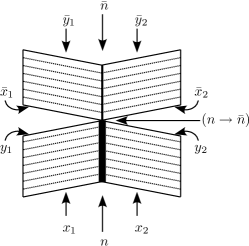
Note that here the analogue to spin foams is not exact, since in a spin foam, the spin labels on each face of the triangulation are constant. In the expansion derived here there is non-trivial dynamics for the ‘spins’, ${\bf x}_{i}$, even with a fixed ‘graph’ $n$. In general there are two distinct labels for a face, those at the beginning, ${\bf x}_{i}$ and those at the end, ${\bf y}_{i}$, and ${\bf y}_{i}\neq{\bf x}_{i}$. Also, in a spin foam there is no restriction on the spins across a vertex, whereas in our case ${\bf y}_{i}$ and ${\bf x}_{i+1}$ (the ‘spin’ labels on either side of the $(i+1)^{\rm th}$ vertex ) are very closely related, by the form of Eq. (21). Thus, although the analogue is not complete, the form of the expansions are qualitatively the same.

III.3 Histories amplitudes

We now discuss how path amplitudes appearing in Eq. (43) can be calculated and illustrate the procedure in the simplest case. The first step is to evaluate the matrix element $\langle{\bf x}_{f}|A(n_{M},\ldots,n_{0};\tau_{M},\ldots,\tau_{1};\alpha)|{\bf x}_{i}\rangle$ of the operator defined in Eq. (33). This operator consist of compositions of operators $A_{n}(\tau)$ and $V_{n^{\prime}n}$, given respectively in Eq. (34) and Eq. (37), which themselves are constructed from translations in the ${\bf x}$ plane. Because of the translation invariance, we will consider the matrix elements between $\langle{\bf x}|$ and $|0\rangle$; the original matrix element is then recovered by the substitution ${\bf x}\to{\bf x}_{f}-{\bf x}_{i}$.

Let us discuss the structure of the operators in more detail. As already noted, $V_{n^{\prime}n}$ vanishes unless $n^{\prime}=n\pm 1$, in which case it is given by Eq. (21). It consist of an overall factor times six simple shifts involving lengths of $a^{\pm}_{n}$ and $a^{\pm}_{n\pm 1/2}$. The $A_{n}(\tau)$ operator is the exponentiation of ($-i\tau$ times) the operator given in Eq. (20). It can be factored into two terms,

$$A_{n}(\tau)=A^{+}_{n}(\tau)A^{-}_{n}(\tau)~{},$$ (45)

where

$$A^{\pm}_{n}(\tau)=e^{-i\tau 2\pi G\,n(2n\pm 1)\left[\cos a^{\pm}_{n}p_{1}+\cos a^{\pm}_{n}p_{2}+\cos(a^{\pm}_{n}p_{2}-a^{\pm}_{n}p_{1})\right]}~{},$$ (46)

which only involves shifts with step-size $a^{\pm}_{n}$. The total operator $A(n_{M},\ldots,n_{0};\tau_{M},\ldots,\tau_{1};\alpha)$ is then a product of operators involving shifts of lengths $a^{\pm}_{j}$ with $j=n_{m}$ or $j=n_{m}\pm 1/2$ ($m=0,\ldots,M$). As a result the matrix element between $\langle{\bf x}|$ and $|0\rangle$ vanishes unless ${\bf x}$ lies in the ‘lattice’ generated by the $a^{\pm}_{j}$ steps. The computation simplifies by selecting among the $a^{\pm}_{j}$’s, a set of independent (i.e. incommensurate) lengths that generate the ‘lattice’.

Let us illustrate the situation by considering the simplest path, namely the $M=0$ case. In this case the amplitude is given by the matrix element $\langle{\bf x}|A_{n}(\tau)|0\rangle$. As already noticed, this operator contains two step-sizes, $a^{+}_{n}$ and $a^{-}_{n}$, and so the nontrivial matrix elements occur whenever ${\bf x}$ lies in the lattice ,

$${\bf x}={\bf k}^{+}a^{+}_{n}+{\bf k}^{-}a^{-}_{n}\ ;\qquad{\bf k}^{+}=(k^{+}_{1},k^{+}_{2})\in\mathbb{Z}^{2},\;{\bf k}^{-}=(k^{-}_{1},k^{-}_{2})\in\mathbb{Z}^{2}~{}.$$ (47)

From the definition of $a^{+}_{n}$ and $a^{-}_{n}$, Eq. (18), one can check that these two numbers are always incommensurate, and so they form an independent set of generators of the lattice. That is to say, a point in the lattice defined by Eq. (47) is uniquely decomposed into its $a^{+}_{n}$ and $a^{-}_{n}$ components, i.e., if ${\bf k}^{+}a^{+}_{n}+{\bf k}^{-}a^{-}_{n}={\bf l}^{+}a^{+}_{n}+{\bf l}^{-}a^{-}_{n}$ then ${\bf k}^{\pm}={\bf l}^{\pm}$.

Thus, the kets $|{\bf x}={\bf k}^{+}a^{+}_{n}+{\bf k}^{-}a^{-}_{n}\rangle$, form a basis of the subspace of vectors which give a non-vanishing matrix element. This space has the structure of a tensor product of two copies of $L^{2}(\mathbb{Z}^{2})$,

$$|{\bf x}={\bf k}^{+}a^{+}_{n}+{\bf k}^{-}a^{-}_{n}\rangle~{}=|{\bf k}^{+}\rangle\otimes|{\bf k}^{-}\rangle$$ (48)

where $|{\bf k}^{+}\rangle$ and $|{\bf k}^{-}\rangle$ are viewed as basis of two abstract $L^{2}(\mathbb{Z}^{2})$ spaces.

Viewed in this way, the $A^{\pm}_{n}(\tau)$ operators act separately on each $L^{2}(\mathbb{Z}^{2})$ factor:

$$\langle{\bf x}={\bf k}^{+}a^{+}_{n}+{\bf k}^{-}a^{-}_{n}|A_{n}(\tau)|0\rangle=\langle{\bf k}^{+}|A^{+}_{n}(\tau)|0\rangle\langle{\bf k}^{-}|A^{-}_{n}(\tau)|0\rangle~{}.$$ (49)

Each factor is the matrix element of a (translation invariant) operator in a single $L^{2}(\mathbb{Z}^{2})$ space, and so can be evaluated by taking the Fourier transform. Using Eq. (20) one finds

$$\langle{\bf k}^{\pm}|A^{\pm}_{n}(\tau)|0\rangle=\int_{0}^{2\pi}\frac{\textrm{d}{\theta_{1}}}{2\pi}\int_{0}^{2\pi}\frac{\textrm{d}{\theta_{2}}}{2\pi}e^{ik^{\pm}_{1}\theta_{1}+ik^{\pm}_{2}\theta_{2}}e^{-i2\pi Gn(2n\pm 1)\tau\left(\cos\theta_{1}+\cos\theta_{2}+\cos(\theta_{2}-\theta_{1})\right)}~{}.$$ (50)

In the general case of a path with $M$ transitions and $g$ independent generators, the space of vectors giving a non-vanishing matrix elements will have now the structure of a tensor product of $g$ copies of $L^{2}(\mathbb{Z}^{2})$. Because the vertex $V_{n^{\prime}n}$ is the sum of six terms, one will generically have a total of $\sim 6^{M}$ terms, each of them involving $g$ Fourier integrals of the type described above. The expressions for these integrals can be directly read off from Eqs. (20) and (21).

After the evaluation of the matrix element $\langle{\bf x}_{f}|A(n_{M},\ldots,n_{0};\tau_{M},\ldots,\tau_{1};\alpha)|{\bf x}_{i}\rangle$, one has to perform the $\tau$ integrals in Eq. (33), and the $p_{\phi}$ and $\alpha$ integrals in Eq. (44). In our $M=0$ case, there are no $\tau$ integrals to perform, and the $\alpha$ integral can be done if interchanged with the Fourier integrals of Eq. (50). This gives a Dirac delta, which in turn allows one to evaluate the integral over $p_{\phi}$. The result is,

$$A(n;{\bf x}_{i},{\bf x}_{f};\phi_{i},\phi_{f})=\int_{D}\frac{\textrm{d}^{4}\theta}{(2\pi)^{4}}e^{i\theta_{1}k^{+}_{1}+\theta_{2}k^{+}_{2}+\theta_{3}k^{-}_{1}+\theta_{4}k^{-}_{2}}e^{i(\phi_{f}-\phi_{i})\sqrt{2\pi Gn}\sqrt{(2n+1)h(\theta_{1},\theta_{2})+(2n-1)h(\theta_{3},\theta_{4})}}~{},$$ (51)

where ${\bf x}_{f}-{\bf x}_{i}={\bf k}^{+}a^{+}_{n}+{\bf k}^{-}a^{-}_{n}$,   $h(\theta_{1},\theta_{2})=\cos\theta_{1}+\cos\theta_{2}+\cos(\theta_{2}-\theta_{1})$ and the domain of integration is

$$D=\{(\theta_{1},\theta_{2},\theta_{3},\theta_{4})\in[0,2\pi)^{4}\;/\,(2n+1)h(\theta_{1},\theta_{2})+(2n-1)h(\theta_{3},\theta_{4})>0\}.$$ (52)

So far we have discussed histories amplitudes of the form $A(n_{M},\ldots,n_{0};{\bf x}_{i},{\bf x}_{f};\phi_{i},\phi_{f})$, where intermediate anisotropies are already summed over. Let us now discuss briefly how one would compute the amplitude for an individual ‘colouring’ of such a history, $A({\bf y}_{M},n_{M},{\bf x}_{M},{\bf y}_{M-1},n_{M-1},\ldots,{\bf y}_{0},n_{0},{\bf x}_{0})$. The building blocks in this case are the amplitudes $A_{n{\bf y}{\bf x}}(\tau)$ and $V_{n^{\prime}{\bf x}n{\bf y}}$, Eq. (41) and Eq. (42). The first amplitude coincides with the $M=0$ case discussed above. We thus have that $A_{n{\bf y}{\bf x}}(\tau)$ vanishes unless ${\bf y}-{\bf x}={\bf k}^{+}a^{+}_{n}+{\bf k}^{-}a^{-}_{n}$ in which case it is given by Eqs. (49) and (50). On the other hand, the value for $V_{n^{\prime}{\bf x}n{\bf y}}$ can be easily read off from its definition: it vanishes unless $n^{\prime}=n\pm 1$ and ${\bf y}-{\bf x}$ lies in one of the following six points, $\{(a^{\pm}_{n},0),(a^{\pm}_{n\pm 1/2},0),(a^{\pm}_{n},a^{\pm}_{n\pm 1/2}),(0,a^{\pm}_{n}),(0,a^{\pm}_{n\pm 1/2}),(a^{\pm}_{n\pm 1/2},a^{\pm}_{n})\}$, in which case it takes the value $-\pi G\sqrt{n(n\pm 1)}(2n\pm 1)$. After multiplying by the remaining factors in Eq. (40), one has to perform the same integrals as previously, in this case given in Eq. (39) and Eq. (44).

III.4 Vacuum case

The presence of matter entered only at the very end of the construction. If we did not have matter at all, we could still follow the same procedure and arrive at the vacuum equivalent of Eq. (43),

$$([n_{f},{\bf x}_{f}],[n_{i},{\bf x}_{i}])=\sum_{M=0}^{\infty}\Big{[}\sum_{n_{M-1},\ldots,n_{1}}A^{\text{vacuum}}(n_{M},\ldots,n_{0};{\bf x}_{i},{\bf x}_{f})\Big{]}~{}.$$ (53)

The difference between the matter and vacuum cases lies only in the form of the amplitudes, which in the vacuum case are formally given by,

$$A^{\text{vacuum}}(n_{0},\ldots,n_{M};{\bf x}_{i},{\bf x}_{f})=\textstyle{\int}_{-\infty}^{\infty}\textrm{d}{\alpha}\,\langle{\bf x}_{f}|A(n_{0},\ldots,n_{M};\alpha)|{\bf x}_{i}\rangle~{}.$$ (54)

These amplitudes can then be evaluated following the strategy given in the previous section, the only difference being the absence of the final integral over $p_{\phi}$. It is not obvious whether the integral in Eq. (54) converges for all paths thus giving a meaningful expansion. Nevertheless, by looking at the generic behaviour of these integral, one finds some evidence that it may converge. For instance, in the constant volume ($M=0$) path, Eq. (54) gives

$$A^{\text{vacuum}}(n;{\bf x}_{i},{\bf x}_{f})=\frac{1}{2\pi Gn}\int\frac{\textrm{d}^{4}\theta}{(2\pi)^{4}}e^{i\theta_{1}k^{+}_{1}+\theta_{2}k^{+}_{2}+\theta_{3}k^{-}_{1}+\theta_{4}k^{-}_{2}}\delta\left((2n+1)h(\theta_{1},\theta_{2})+(2n-1)h(\theta_{3},\theta_{4})\right)~{}$$ (55)

which is clearly finite (at least for $n>0$). This is to be contrasted with the vacuum FRW case ach2 , and the example in rv2 , where a regulator is required in order to render finite the otherwise divergent amplitudes, even in this $M=0$ case. Further study of the vacuum case is in progress Ed_Adam .

IV Projection to FRW

At the end of section II, we commented on the projection from Bianchi I to FRW. We show here that when such projection is done at the level of the vertex expansion, Eq (43), one recovers the FRW vertex expansion of ach2 .

The structure in both cases is almost identical. One has a sum over volume sequences $(n_{M},\ldots,n_{0})$, and each amplitude is constructed by first obtaining a gravitational amplitude, and then performing the group averaging and scalar field integrations. Thus, all that remains is to show that the amplitude $\langle{\bf x}_{f}|A(n_{M},\ldots,n_{0};\tau_{M},\ldots,\tau_{1};\alpha)|{\bf x}_{i}\rangle$ given in Eq. (33) projects to the corresponding FRW one,

$$A^{\text{FRW}}(n_{M},\ldots,n_{0};\tau_{M},\ldots,\tau_{1};\alpha)= \;e^{-i(\alpha-\tau_{M})\Theta^{\text{FRW}}_{n_{M}n_{M}}}\,\,\Theta^{\text{FRW}}_{n_{M}n_{M-1}}\,\,\times$$

$$\ldots\,\,e^{-i(\tau_{2}-\tau_{1})\Theta^{\text{FRW}}_{n_{1}n_{1}}}\,\,\Theta^{\text{FRW}}_{n_{1}n_{0}}\,\,e^{-i\tau_{1}\Theta^{\text{FRW}}_{n_{0}n_{0}}}~{},$$ (56)

when summing over all possible values of ${\bf x}_{f}$.

To show this, it is convenient to explicitly write the intermediate anisotropies in the amplitude $\langle{\bf x}_{f}|A(n_{M},\ldots,n_{0};\tau_{M},\ldots,\tau_{1};\alpha)|{\bf x}_{i}\rangle$. As before, this is done by introducing complete basis $\mathbf{1}_{\lambda}=\sum_{{\bf x}_{m}}|{\bf x}_{m}\rangle\langle{\bf x}_{m}|$ and $\mathbf{1}_{\lambda}=\sum_{{\bf y}_{m}}|{\bf y}_{m}\rangle\langle{\bf y}_{m}|$ to the right and left of the $A_{n_{m}}(\tau_{m+1}-\tau_{m})$ operator in Eq. (33). Calling ${\bf x}_{f}\equiv{\bf y}_{M}$ and ${\bf x}_{i}\equiv{\bf x}_{0}$ we have,

$$\sum_{{\bf y}_{M}}\langle{\bf y}_{M}|A(n_{M},\ldots,n_{0};\tau_{M},\ldots,\tau_{1};\alpha)|{\bf x}_{0}\rangle=\sum_{\begin{subarray}{c}{\bf x}_{1},\ldots,{\bf x}_{M}\\ {\bf y}_{0},\ldots,{\bf y}_{M}\end{subarray}}\langle{\bf y}_{M}|A_{n_{M}}(\alpha-\tau_{M})|{\bf x}_{M}\rangle$$

$$\langle{\bf x}_{M}|V_{n_{M}n_{M-1}}|{\bf y}_{M-1}\rangle\langle{\bf y}_{M-1}|A_{n_{M-1}}(\tau_{M}-\tau_{M-1})|{\bf x}_{M-1}\rangle\ldots\langle{\bf x}_{1}|V_{n_{1}n_{0}}|{\bf y}_{0}\rangle\langle{\bf y}_{0}|A_{n_{0}}(\tau_{1})|{\bf x}_{0}\rangle~{}.$$ (57)

We now use the translation invariance of the operators to write each matrix elements in Eq. (IV) as $\langle{\bf x}^{\prime}|f|{\bf x}\rangle=\langle{\bf x}^{\prime}-{\bf x}|f|0\rangle$ where $f$ is either the $A$ or $V$ operators. We then change the summation variables to ${\bf y}^{\prime}_{m}={\bf y}_{m}-{\bf x}_{m}$ and ${\bf x}^{\prime}_{m}={\bf x}_{m}-{\bf y}_{m-1}$. The different summations in Eq. (IV) then decouple giving,

$$\sum_{{\bf y}_{M}}\langle{\bf y}_{M}|A(n_{M},\ldots,n_{0};\tau_{M},\ldots,\tau_{1};\alpha)|{\bf x}_{0}\rangle=\left(\sum_{{\bf y}^{\prime}_{M}}\langle{\bf y}^{\prime}_{M}|A_{n_{M}}(\alpha-\tau_{M})|0\rangle\right)\left(\sum_{{\bf x}^{\prime}_{M}}\langle{\bf x}^{\prime}_{M}|V_{n_{M}n_{M-1}}|0\rangle\right)$$

$$\left(\sum_{{\bf y}^{\prime}_{M-1}}\langle{\bf y}^{\prime}_{M-1}|A_{n_{M-1}}(\tau_{M}-\tau_{M-1})|{\bf x}_{M-1}\rangle\right)\ldots\left(\sum_{{\bf x}^{\prime}_{1}}\langle{\bf x}^{\prime}_{1}|V_{n_{1}n_{0}}|0\rangle\right)\left(\sum_{{\bf y}^{\prime}_{0}}\langle{\bf y}^{\prime}_{0}|A_{n_{0}}(\tau_{1})|0\rangle\right)~{}.$$ (58)

Comparing Eq. (IV) and Eq. (IV) we see that our task reduces to showing that $\sum_{\bf x}\langle{\bf x}|A_{n}(\tau)|0\rangle=e^{-i\tau\Theta^{FRW}_{nn}}$ and $\sum_{\bf x}\langle{\bf x}|V_{n^{\prime}n}|0\rangle=\Theta^{FRW}_{n^{\prime}n}$. That this is so can be seen as a direct consequence of the result in awe . Let us nevertheless show it explicitly.

For the $V$ term, it suffices to look at $V_{n\pm 1n}$. The operator, given in Eq. (21) consist in an overall constant times six different translations in the ${\bf x}$ plane. Each term thus will pick up a single ${\bf x}$ from the sum. For instance, the first term gives a nonzero value only for ${\bf x}=(a^{\pm}_{n},0)$, in which case it gives a contribution of $-\pi G\sqrt{n(n\pm 1)}(2n\pm 1)$. We then conclude that

$$\sum_{{\bf x}}\langle{\bf x}|V_{n\pm 1n}|0\rangle=-6\pi G\sqrt{n(n\pm 1)}(2n\pm 1)=\Theta^{FRW}_{n\pm 1n}~{},$$ (59)

as required.

For the $A_{n}(\tau)$ term we have

$$\sum_{\bf x}\langle{\bf x}|A_{n}(\tau)|0\rangle=$$

$$\sum_{{\bf k}^{+},{\bf k}^{-}\in\mathbb{Z}^{2}}\langle{\bf k}^{+}|A^{+}_{n}(\tau)|0\rangle\langle{\bf k}^{-}|A^{-}_{n}(\tau)|0\rangle=$$

$$e^{-i\tau 24\pi Gn^{2}}=e^{-i\tau\Theta^{FRW}_{nn}}~{},$$ (60)

where in going from the first to second line, we used Eq. (49). In going from the second to third line, we used Eq. (50) and the identity $\sum_{k\in\mathbb{Z}}e^{ik\theta}/2\pi=\delta(\theta)$ to directly evaluate the Fourier integrals. Using Eqs. (59) and (IV) we then have

$$\sum_{{\bf x}_{f}}\langle{\bf x}_{f}|A(n_{M},\ldots,n_{0};\tau_{M},\ldots,\tau_{1};\alpha)|{\bf x}_{i}\rangle=A^{\text{FRW}}(n_{M},\ldots,n_{0};\tau_{M},\ldots,\tau_{1};\alpha)~{},$$ (61)

which implies

$$\sum_{{\bf x}_{f}}A(n_{M},\ldots,n_{0};{\bf x}_{i},{\bf x}_{f};\phi_{i},\phi_{f})=A^{\text{FRW}}(n_{M},\ldots,n_{0};\phi_{i},\phi_{f})~{}.$$ (62)

Thus we see that the vertex expansion for our Bianchi model, Eq. (43) projects down to the vertex expansion of the FRW model, order by order.

V Discussion

Recently it has been shown ach1 that one can take the Loop Quantum version of FRW cosmology and expand it as a sum over volume transition of amplitudes compatible with given initial and final states i.e. that the cosmological model of Loop Quantum Gravity can be re-written in terms of a sum over amplitudes, analogous to the spin foam approach. This sum over transition amplitudes is produced as a perturbation expansion of the constraint operator of LQC, thus linking perturbative dynamics of LQC to (the analogue of) spin foams. This analogue provided a useful link between the two theories, however because there is only one dynamic parameter in FRW cosmologies – the volume – the system has no analogue of the spin labels. In this paper we have extended the approach of ach1 to the Bianchi I cosmological model, which, in addition to volume, has anisotropic degrees of freedom. We have shown that it is again possible to expand the dynamics of the model in terms of sums of amplitudes over volume transitions compatible with initial and final states. The additional anisotropic degrees of freedom of this model are analogous to the spin labels of spin networks, thus significantly improving the analogue to spin foams.

The analogue remains at a formal level however, because one cannot directly associate the amplitudes with the changing of an underlying spin network. Despite this the association of the anisotropic degrees of freedom with the spin labels is well motivated by the fact that in LQC they give the area (of the fiducial cell), which is precisely the role played by the spin labels (and edges) in a spin network. In addition to showing that the resulting summation over ‘spin’ labels is finite, we show that the projection to the FRW system occurs order by order in the expansion, thus recovering the results of ach1 .

Finally, although spin foams are typically taken to have spin changes only at vertices, it is generally expected that spin dynamics in the absence of graph changing vertices will play an important role in the final theory freidel . More precisely, that the action of the full constraint is non-trivial, even in the absence of vertices and hence that the amplitude for each vertex-free segment of the spin foam will be non-diagonal in the spin labels. In the analogue produced here we show that indeed the ‘spin’ changing amplitude is non-trivial, even in the absence of volume changing ‘vertices’. Thus our full expansion is the analogue of a generalization of spin foams, allowing for ‘spin’ dynamics.

References

- (1) A. Ashtekar, M. Campiglia and A. Henderson, Loop quantum cosmology and spin foams, Phys. Lett. B681,347-352 (2009)
- (2) A. Ashtekar, M. Campiglia and A. Henderson, Casting Loop Quantum Cosmology in the Spin Foam Paradigm, Class. Quant. Grav. 27, 135020 (2010)
- (3) A. Ashtekar and J. Lewandowski, Background independent quantum gravity: A status report, Class. Quant. Grav. 21, R53-R152 (2004)
- (4) C. Rovelli,Quantum Gravity. (Cambridge University Press, Cambridge (2004))
- (5) C. Rovelli, Loop Quantum Gravity, Living Reviews in Relativity, (2008).
- (6) T. Thiemann, Introduction to Modern Canonical Quantum General Relativity. (Cambridge University Press, Cambridge, (2007))
- (7) J. Baez, An introduction to spinfoam models of BF theory and quantum gravity, Lect.Notes Phys. 543 25-94 (2000)
- (8) A. Perez, Introduction to loop quantum gravity and spin foams, arXiv:gr-qc/0409061
- (9) C. Rovelli, A new look at loop quantum gravity, arXiv:1004.1780
- (10) Y. Ding and C. Rovelli, Physical boundary Hilbert space and volume operator in the Lorentzian new spin-foam theory, arXiv:1006.1294
- (11) J. Engle and R. Pereira, Coherent states, constraint classes, and area operators in the new spin-foam models, Class. Quant. Grav. 25, 105010 (2008)
- (12) W. Kaminski,M. Kisielowski and J. Lewandowski, Spin-Foams for All Loop Quantum Gravity, Class. Quant. Grav. 27, 095006 (2010)
- (13) M. P. Reisenberger and C. Rovelli, Sum over surfaces form of loop quantum gravity, Phys. Rev. D56, 3490-3508 (1997)
- (14) K. Noui and A. Perez, Three dimensional loop quantum gravity: Physical scalar product and spin foam models, Class. Quant. Grav. 22, 1739-1762 (2005)
- (15) M. Bojowald, Loop Quantum Cosmology, Living Reviews in Relativity (2008)
- (16) E. Bianchi, C. Rovelli and F. Vidotto, Towards Spinfoam Cosmology, arXiv:1003.3483
- (17) C. Rovelli and F. Vidotto, Stepping out of Homogeneity in Loop Quantum Cosmology, Class. Quant. Grav. 25, 225024 (2008)
- (18) K. Noui, A. Perez and K. Vandersloot, Cosmological Plebanski theory, Gen. Rel. Grav. 41, 2597-2618 (2009)
- (19) A. Ashtekar and E. Wilson-Ewing, Loop quantum cosmology of Bianchi type I models, Phys. Rev. D79, 083535 (2009)
- (20) A. Ashtekar, A. Corichi and P. Singh, Robustness of predictions of loop quantum cosmology, Phys. Rev. D77, 024046 (2008)
- (21) W. Nelson and M. Sakellariadou, Lattice Refining Loop Quantum Cosmology from an Isotropic Embedding of Anisotropic Cosmology, Class. Quant. Grav. 27, 145014 (2010)
- (22) C. Rovelli and F. Vidotto, On the spinfoam expansion in cosmology, Class. Quant. Grav. 27, 145005 (2010).
- (23) A. Henderson and E. Wilson-Ewing, in preperation
- (24) L. Freidel (personal communication to A. Henderson)