MASSCLEANage
– Stellar Cluster Ages from Integrated Colors –

Abstract

We present the recently updated and expanded MASSCLEANcolors, a database of 70 million Monte Carlo models selected to match the properties (metallicity, ages and masses) of stellar clusters found in the Large Magellanic Cloud (LMC). This database shows the rather extreme and non-Guassian distribution of integrated colors and magnitudes expected with different cluster age and mass and the enormous age degeneracy of integrated colors when mass is unknown. This degeneracy could lead to catastrophic failures in estimating age with standard SSP models, particularly if most of the clusters are of intermediate or low mass, like in the LMC. Utilizing the MASSCLEANcolors database, we have developed MASSCLEANage, a statistical inference package which assigns the most likely age and mass (solved simultaneously) to a cluster based only on its integrated broad-band photometric properties. Finally, we use MASSCLEANage to derive the age and mass of LMC clusters based on integrated photometry alone. First we compare our cluster ages against those obtained for the same seven clusters using more accurate integrated spectroscopy. We find improved agreement with the integrated spectroscopy ages over the original photometric ages. A close examination of our results demonstrate the necessity of solving simultaneously for mass and age to reduce degeneracies in the cluster ages derived via integrated colors. We then selected an additional subset of 30 photometric clusters with previously well constrained ages and independently derive their age using the MASSCLEANage with the same photometry with very good agreement. The MASSCLEANage program is freely available under GNU General Public License.

Accepted for publication in The Astrophysical Journal

1 Introduction

Stellar clusters are among the most universally-useful entities studied by modern day astronomers. Having a set of singly-aged, same-distance stars in an identifiable cluster provides stellar and galactic astronomers with powerful diagnostic tools to interpret our universe. Of particular interest is the ability to use the ages and masses of constituent stellar clusters to track the star formation history and chemical evolution of a galaxy, the mass function of stellar clusters and their lifetime within differing galaxies (e.g. Lamers et al. 2005; Piatti et al. 2009; Larsen 2009; Mora et al. 2009; Chandar et al. 2010a). However, such measures require deriving the ages and masses of stellar clusters when the constituent stars within those clusters are not individually resolved. With distant stellar clusters, one has only the integrated properties to work from, typically in either broad band photometry or integrated spectroscopy, to estimate ages (e.g. Searle et al. 1980; van den Bergh 1981). In such cases, we rely on sophisticated models of these star systems to derive the cluster properties (age, mass, chemistry) based on their observed, bulk properties. For this reason there exists a long history of effort interpreting integrated cluster properties through the use of these sophisticated models (e.g. Girardi et al. 1995; Bruzual & Charlot 2003; Cerviño & Valls-Gabaud 2009; Buzzoni 1989; Chiosi 1989; Bruzual 2002; Bruzual 2010; Cerviño & Luridiana 2004; Cerviño & Luridiana 2006; Fagiolini et al. 2007; Lançon & Mouhcine 2000; Lançon & Fouesneau 2009; Fouesneau & Lançon 2009; Fouesneau & Lançon 2010; Brocato et al. 1999; Brocato et al. 2000; Cantiello et al. 2003; Raimondo et al. 2005; Raimondo 2009; Santos et al. 2006; González et al. 2004; González-Lópezlira et al. 2005; González-Lópezlira et al. 2010; Maíz Apellániz 2009; Pessev et al. 2009; Popescu & Hanson 2010b).

Quite recently, we presented our own independent effort to provide models for interpreting integrated stellar cluster photometry. Our model, MASSCLEAN (MASSive CLuster Evolution and ANalysis – Popescu & Hanson 2009), is rather unique in its design compared to other stellar cluster models and provides additional insight to interpreting presently available data on stellar clusters. In this paper we first present in §2 our recently expanded data-set of 70 million Monte Carlo models, MASSCLEANcolors (Popescu & Hanson 2010a). This database of models shows the stochastic and non-Gaussian behavior of integrated stellar cluster colors and magnitudes as a function of cluster mass and age. This, our first, newly completed, extended database of models, was selected to match the mass, age and metallicity range expected in the stellar clusters of the Large Magellanic Cloud (LMC). In §3, we demonstrate the utility of this extensive database. When used with a statistical inference code we have designed within MASSCLEAN called, MASSCLEANage, we use the database to work backwards from the integrated magnitudes and colors of real LMC clusters, to derive their stellar ages and masses. We also discuss our new age results as compared to previous age determinations based on the same photometric data, to provide initial tests on the cluster results obtained using MASSCLEANage. Final discussion of our results and conclusions are found in §4.

2 The MASSCLEANcolors Database – Now Over 70 Million Monte Carlo Simulations

We have computed the integrated colors and magnitudes as a function of mass and age for a simple stellar cluster. Our results – the newest version of the MASSCLEANcolors database (Popescu & Hanson 2010a) – are based on over $70$ million Monte Carlo simulations using Padova 2008 (Marigo et al. 2008) and Geneva (Lejeune & Schaerer 2001) isochrones, and for two metalicities, $Z=0.019$ (solar) and $Z=.008$ (LMC). The simulation were done using Kroupa IMF (Kroupa 2002) with $0.1$ $M_{\sun}$ and $120$ $M_{\sun}$ mass limits. The age range of $[6.6,9.5]$ in $log(age/yr)$ was chosen (similar to Popescu & Hanson 2009; Popescu & Hanson 2010a) to accomodate both Padova and Geneva models. The mass range is $200$-$100,000$ $M_{\sun}$. An average of $5000$ clusters were simulated for each mass and age.

In this work we will look closely at a subset of the MASSCLEANcolors database. We present integrated magnitudes and colors ($M_{V}$, $(U-B)_{0}$, $(B-V)_{0}$) representing 50 million Monte Carlo simulations using Padova 2008 stellar evolutionary models alone and for the single metallicity, $Z=.008$ ([Fe/H]=-0.6), selected to match the bulk properties of the LMC over most of the past few billion years (Piatti et al. 2009).

2.1 The Distribution of Integrated Colors and Magnitudes as a Function of Mass and Age

In Popescu & Hanson 2010a, we analysed the influence of the stochastic fluctuations in the mass function of stellar clusters on their integrated colors as a function of cluster mass. Using 13 mass intervals ranging from 500–100,000 $M_{\sun}$, we showed the mean value of the distribution of integrated colors varies with mass. We further showed that the dispersion of integrated colors, measured by $1\sigma$ (standard deviation), increases as the value of the cluster mass decreases. In this new work we will present not just the sigma range and mean, but the full distribution of integrated colors and magnitudes. We are also using a much larger number of Monte Carlo simulations and cluster mass values in the 200–100,000 $M_{\sun}$ interval. This allows us to look closely at where the distribution of real cluster properties lie in the critical color-age and color-color diagrams.

The distribution of integrated $M_{V}$ magnitudes as a function of mass and age is presented in the upper panel of Figure 1. The corresponding mass values are color-coded and presented in the bottom panel. Sixty-five (65) different mass intervals have been explored in the MASSCLEANcolors database as part of this demonstration. All 65 mass intervals are plotted on top of each other, making it difficult to see the individual distributions. However, to first order, higher mass clusters have higher absolute magnitudes, $M_{V}$.

In Figures 2 and 3 we present the distribution of $(B-V)_{0}$ and $(U-B)_{0}$ integrated colors as a function of mass and age. The mass values are represented by the same colors as shown in the bottom panel of Figure 1. The variation of integrated colors computed in the infinite mass limit ($10^{6}$ $M_{\sun}$ in our simulations) and consistent with standard simple stellar population (SSP) models based on Padova 2008 (Marigo et al. 2008), is represented by the solid white line in both figures. As was shown in Popescu & Hanson 2010a, the dispersion in integrated colors grows larger for lower mass clusters, both in the blue and red side. As the cluster mass increases, the dispersion decreases and the integrated colors approach the infinite mass limit shown in white. While it is valuable to see the range of masses over-layed in a single plot, it is difficult to see the exact shape of the color distributions underlying each mass interval.

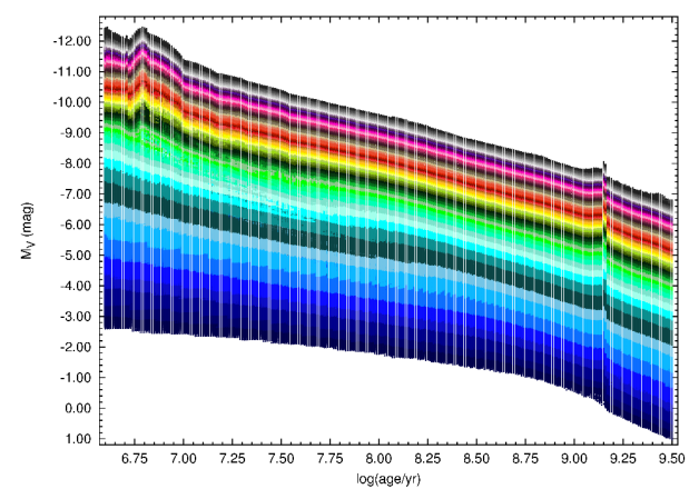
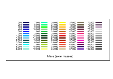
Figure 1: The results from 50 million Monte Carlo simulations created with MASSCLEAN. Models were generated with 65 different masses and evolved following Padova 2008 evolutionary models. Higher mass clusters are plotted over preceded lower mass clusters. This figure gives the (partially correct) impression that $M_{V}$ monotonically increases with cluster mass for all ages.

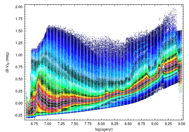
Figure 2: The results from the same 50 million Monte Carlo simulations as shown in Figure 1 and using the same color coding to represent cluster mass. The range of $(B-V)_{0}$ colors, as a function of mass and age is given. Again, higher mass clusters are plotted over preceded lower mass clusters, so covers the real distribution of expected colors as a function of mass and age. A white line which lies at the color center, represents the color dependence with age computed in the infinite mass limit ($10^{6}M_{\sun}$ in our simulations). This figure gives the (correct) impression that the range of cluster colors observed as a function of age, is greatly increased for lower mass clusters.

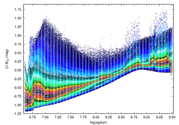
Figure 3: The same as Figure  2, only this figure shows $(U-B)_{0}$ colors as a function of mass and age.

2.2 The Shape of the Distribution of Integrated Colors and Magnitudes

We have selected a few single values of mass for independent plots in Figures 4–6. The distribution of integrated $M_{V}$ magnitudes is presented in Figure 4, for clusters mass of 200, 1,000, 5,000, 10,000, 25,000, and 50,000 $M_{\sun}$, respectively. The colors are the same as the ones used in Figure 1. What is also given in a black line is the mean value of the distribution of integrated $M_{V}$ magnitudes for that mass (Popescu & Hanson 2010a). Several very critical effects are immediately apparent. The distribution (range) of observed integrated magnitudes for low mass clusters gets very large with lower mass clusters. This was already presented in Popescu & Hanson 2010a. However, the shape of that dispersion was not presented like we have done here. Here we see in Fig. 4, particularly with 200 and 1,000 solar mass clusters, the distribution becomes bimodal for the lowest mass clusters, especially for young ages (log t $\leq$ 8.0). A cluster with no more than 200 solar masses can, at times, have an absolute magnitude typical of a cluster $25-100$ times more massive and at the same age. Even if one can derive an accurate age for their cluster, one can not rely on the absolute magnitude alone to derive mass unambiguously.

In Figures 5 and 6 we present the distribution of integrated colors $(B-V)_{0}$ and $(U-B)_{0}$ as a function of age for the same select values of cluster mass, 200, 1,000, 5,000, 10,000, 25,000, and 50,000 $M_{\sun}$, respectively. The integrated colors as a function of age, computed in the infinite mass limit ($10^{6}M_{\sun}$ in our simulations) is represented by the solid black line. Here the structure in the values observed start out closely aligned with the classical SSP codes predictions (infinite mass limit) for the high mass clusters, but quickly fans out to a rather broad distribution below 10,000 $M_{\sun}$. When one gets below 1,000 $M_{\sun}$, the color range is extreme, both in the red and blue colors predicted by our models. Moreover, the distribution shows a clear bimodal distribution (Popescu & Hanson 2010a; Lançon & Mouhcine 2002; Cerviño & Luridiana 2004; Fagiolini et al. 2007). In Popescu & Hanson 2010a, we discussed the increased dispersion in colors as the cluster mass decreased, though we did not investigate masses as low as shown here. However, even clusters with masses of 1,000 to as much as 5,000 $M_{\sun}$ show an extraordinary range in colors, away from the predicted SSP single expectation value with age.

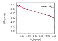
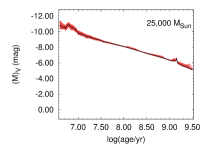
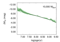
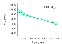
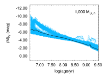
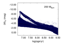
Figure 4: Beginning in the upper left panel, the black line shows the mean value of the distribution of integrated $M_{V}$ colors for a 50,000 $M_{\sun}$ cluster. The red points are MASSCLEAN, Monte Carlo derived observed magnitudes for a 50,000 $M_{\sun}$ cluster, as a function of age. Over one million models are used to derive the red points in this figure. The distribution seen about the mean value is relatively small. In the next panel to the right, is given the magnitudes, as a function of age, for Monte Carlo derived cluster with mass, 25,000 $M_{\sun}$. The black line is the mean value of the distribution of integrated $M_{V}$ colors for a 25,000 $M_{\sun}$ cluster. In the following 4 subfigures, we provide lower and lower mass simulated clusters, 10,000 (upper right), then 5,000 (lower left), 1,000 (lower center) and finally 200 $M_{\sun}$ (lower right), all the while showing the mean value of the distribution of integrated $M_{V}$ colors for the corresponding clusters mass. For clusters with masses of only a few thousand solar mass, the observed range becomes extremely large, and can even mimic clusters of lower or even considerably higher total mass.

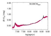
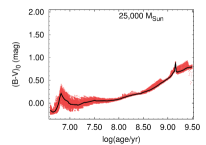
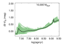
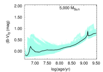
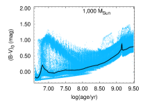
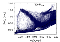
Figure 5: Like with Figure 4, we have selected six mass examples (50,000, 25,000, 10,000, 5,000, 1000, and 200 $M_{\sun}$) to show the observed distribution of $(B-V)_{0}$ colors as a function of age, compared to the infinite mass limit (in the black line, the same for all six plots). For the higher mass clusters, 50,000 and 25,000 $M_{\sun}$, the range of colors is small and stays reasonably close to the values computed in the infinite mass limit. However, in the remaining panels one sees that the observed values from our simulations can demonstrate rather extreme colors, bluer, but more so very red colors at times, for increasingly lower mass clusters.

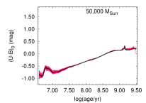
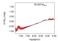
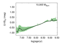
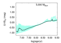
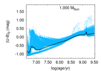
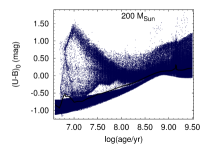
Figure 6: This is the same as for Figure 5, only here we show the variation with mass and age of $(U-B)_{0}$ colors, as derived through Monte Carlo simulations using MASSCLEAN.

2.3 The Distribution of Integrated Colors in the Color-Color Diagram

All the data from Figures 2 and 3 are again presented in Figure 7 as a $(U-B)_{0}$ vs. $(B-V)_{0}$ color-color diagram. And, once again, the variation of integrated colors computed in the infinite mass limit (as predicted by classical SSP codes) is represented by the solid white line. The 65 masses given are color-coded similarly to Figure 1. Provided the mass of the cluster is greater than 50,000 $M_{\sun}$ (in the pink), the predicted properties of our Monte Carlo generated clusters stays reasonably close to the integrated colors computed in the infinite mass limit. For clusters with masses less than 10,000 $M_{\sun}$ (the dark green just beyond the yellow), the range of possible colors becomes quite large, overlapping heavily with many different aged clusters and causing enormous degeneracy problems.

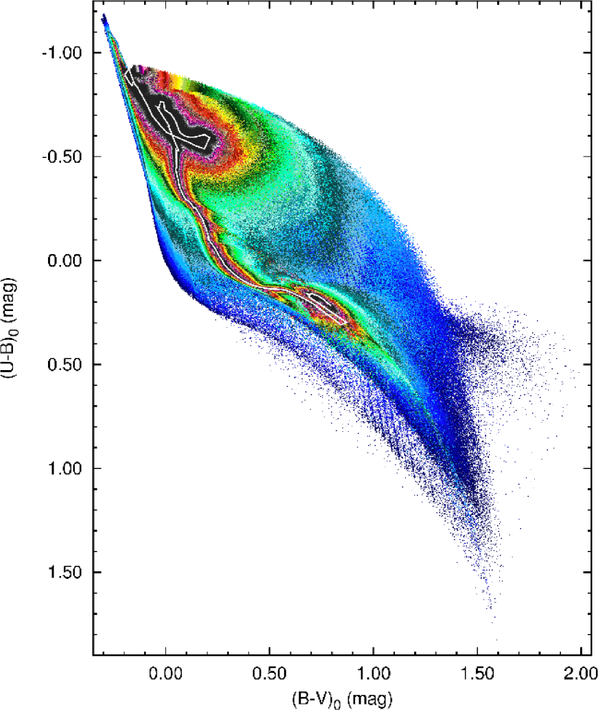
Figure 7: The result of 50 million Monte Carlo simulations, color coded by mass as described in Figure 1. Here we see the full range of color-color magnitudes predicted as a function of mass. Clusters more massive than 50,000 $M_{\sun}$ (in the pink) typically adhere closely to the predicted values for the single solution Padova-based SSP predictions, computed in the infinite mass limit. However, clusters with masses below 10,000 $M_{\sun}$ (the dark green just beyond the yellow) can show extreme color ranges.

The classical method for cluster age determination using integrated colors is based mainly on the $(U-B)_{0}$ vs. $(B-V)_{0}$ color-color diagram. The large dispersion presented in Figure 7 shows the limitation of this method when only the infinite mass limit is used. To better view what is happening in the complex Figure 7, we show another view of this data in Figure 8. Here, we apply an entirely new color scheme to represent our Monte Carlo simulations. In Figure 8 we plot the color-color diagram for 5 ages ($log(age/yr)$= 7.00, 7.50, 8.00, 8.50, 9.00) and all values of mass between 200–100,000 $M_{\sun}$. Clusters of all masses are shown now color coded based on age. Combining this with what we have learned from Figure 7, Figure 8 shows us that even very young low mass clusters can mimic the UBV colors of more massive old clusters. The extreme tail of colors belongs solely to intermediate and low mass clusters. It is easy to see that very young clusters ($log(age/yr)$= 7.00, 7.50) could be mistaken for 1 billion years old ($log(age/yr)$= 9.00) clusters, based on the single SSP relationship in a classical UBV diagram.

The $(U-B)_{0}$ versus $(B-V)_{0}$ color-color diagram is a very important tool in age determination of stellar clusters. The high level of dispersion shown in Figures 7 and 8 demonstrates the limitations of this method when only the infinite mass limit is used. The degeneracy seems to be so extreme, one might think all is lost. But in fact, the purpose of our extensive database was not just to show the range and degeneracy of the colors with age and mass (and here we have only limited ourselves to a single IMF, chemistry and evolutionary model), but to see if by producing such a database, we might provide a reasonable grid of properties from which to work back and derive cluster ages and masses.

2.4 Mass and Age Are Degenerate Quantities in UBV Colors

Figures 1 through 8 demonstrate the very difficult condition one faces in deriving unique ages of stellar clusters when mass is not given full consideration. In creating the MASSCLEANcolors database, we have created a distribution function of observed photometric properties with age and mass. Our figures demonstrate just the UBV bands, however, our MASSCLEANcolors database includes all photometric bands presently included in the Padova 2008 model release: UBVRIJHK. While our figures seem to indicate there is little to match on, in fact, when simultaneously solving all three unique values of UBV ($U-B$, $B-V$ and $M_{V}$) , there will be optimized, or most likely solutions when one searches in both age and mass grid space. If additional photometric bands are available for a cluster, this can be further used to constrain the cluster properties. The module which will provide such a search we call MASSCLEANage.

3 Age Determination for Stellar Clusters – MASSCLEANage

The newest addition to the MASSCLEAN package (Popescu & Hanson 2009) is MASSCLEANage, a program which uses the MASSCLEANcolors database (Popescu & Hanson 2010a) to determine the ages of stellar clusters.

Our program, MASSCLEANage, is based on a method analogous to $\chi^{2}$ minimization. Based on the observational data, integrated magnitude and integrated colors, it searches for the minimum hyper-radius in the integrated magnitude, integrated colors, age, and mass hyperspace. This work specifically is based on a $M_{V}$, $(U-B)_{0}$, $(B-V)_{0}$, age, and mass hyperspace due to the availability of integrated $UBV$ colors and magnitudes from Hunter et al. 2003, but the code can provide results based on more colors. The most probable values for age and mass are reported, along with a list of other possible matches. The number of possible matches could be selected by the user or could be automatically computed based on the photometric errors. The results could be used to generate the confidence levels for age and mass (as presented in Tables 1 and 2 and Figure 9), or to generate the age-mass probability distributions (as presented in Figure 10).

By including additional bands (e.g. $(V-K)_{0}$) the accuracy in the age and mass determination would increase, and could minimize the degeneracies. In order to do it, a much larger version of the database is required, since the range of stochastic fluctuations is much larger in $(V-K)_{0}$ (Popescu & Hanson 2010a).

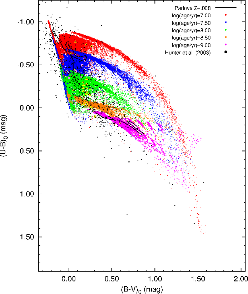
Figure 8: Monte Carlo cluster simulations colored by age for $log(age/yr)=7.00,7.50,8.00,8.50,9.00$. Here we show that young clusters of low mass can be found to reside in the region that the infinite mass limit predict for old stellar clusters. For a comparison with the observational data, the clusters from Hunter et al. 2003 catalog are displayed as black dots. The clusters with photometric ages from Santos et al. 2006 (also presented in Table 1) are highlighted with pink squares. All the clusters presented in Table 2 are highlighted with yellow triangles.

3.1 Age and Mass Determination for LMC Clusters

As a first demonstration of the MASSCLEANage code, we compare our values of ages for 7 clusters with both spectroscopic ages (Santos et al. 2006) and photometric ages (Hunter et al. 2003). Our results are computed using the previously de-reddened values of $M_{V}$, $(U-B)_{0}$, and $(B-V)_{0}$ from the Hunter et al. 2003 catalog. The data is presented in Table 1. The integrated photometry and age from Hunter et al. 2003 is presented in the columns 2–5, and the spectroscopic ages from Santos et al. 2006 is presented in the column 6. The MASSCLEANage results are presented in the columns 7–9. The same data is also presented in Figure 9 (a), (b). The integrated $(U-B)_{0}$ and $(B-V)_{0}$ colors are presented in Figure 8 as pink squares.

The ages computed using MASSCLEANage are in good agreement with the spectroscopic ages from Santos et al. 2006. One object in Figure 9 still lies significantly away from the predicted age, as derived by Santos et al. 2006, even using MASSCLEANage. We investigated a few of the sources in this diagram by looking closely at the minimization solutions found within the MASSCLEANage hyperspace. Absolutely every mass and age range available was specifically calculated against the observed UBV colors. This output was used to create the likelihood plots shown in Figure 10. These banana-shaped diagrams demonstrate the very strong degeneracy in UBV colors between age and mass. Here we see that for NGC 1894, which represents the most significantly desperate point found in Figure 9 (b), our best solution for the age does not match that derived by Santos et al. 2006 via integrated spectroscopy, but agrees with the age from Hunter et al. 2003. If the older Santos et al. 2006 age is correct, then this cluster is fairly massive ($\geq$ 15,000 $M_{\sun}$ based on Figure 10).

Table 1: Results

	Integrated Photometry				Spectroscopy			MASSCLEAN
Name	$M_{V}$	$(U-B)_{0}$	$(B-V)_{0}$	Age		Age		Age	Age	Mass
	$(mag)$	$(mag)$	$(mag)$	$(Myr)$		$(Myr)$		$(Myr)$	$(log)$	$(M_{\sun}$)
$1$	$2$	$3$	$4$	$5$		$6$		$7$	$8$	$9$
NGC 1804	$-6.493$	$-0.523$	$-0.103$	$19.1\pm 7.21$		$60\pm 20$		$29.51^{+15.16}_{-11.73}$	$7.47^{+0.18}_{-0.22}$	$2,000^{+2,000}_{-1,300}$
NGC 1839	$-7.087$	$-0.347$	$0.002$	$16.2\pm 7.16$		$90\pm 30$		$72.44^{+18.76}_{-32.63}$	$7.86^{+0.10}_{-0.26}$	$8,000^{+2,000}_{-4,000}$
SL 237	$-6.951$	$-0.494$	$0.156$	$15.2\pm 7.02$		$40\pm 20$		$38.90^{+10.07}_{-13.78}$	$7.59^{+0.10}_{-0.19}$	$5,000^{+1,000}_{-3,000}$
NGC 1870	$-7.493$	$-0.423$	$0.082$	$15.8\pm 7.54$		$60\pm 30$		$43.65^{+23.96}_{-8.98}$	$7.64^{+0.19}_{-0.10}$	$8,000^{+4,000}_{-2,000}$
NGC 1894	$-7.956$	$-0.550$	$0.192$	$15.0\pm 8.02$		$100\pm 30$		$20.89^{+14.59}_{-1.40}$	$7.32^{+0.23}_{-0.03}$	$7,000^{+5,000}_{-1,000}$
NGC 1913	$-7.547$	$-0.493$	$0.257$	$14.6\pm 7.72$		$40\pm 20$		$33.11^{+11.55}_{-9.12}$	$7.52^{+0.13}_{-0.14}$	$7,000^{+2,000}_{-2,000}$
NGC 1943	$-7.255$	$-0.359$	$0.137$	$15.5\pm 7.31$		$140\pm 60$		$79.43^{+7.66}_{-31.57}$	$7.90^{+0.04}_{-0.22}$	$10,000^{+1,000}_{-4,000}$

Figure 9: In (a) above, the $log(age/yr)$ as derived by Hunter et al. (2003) using UBV photometry alone is shown versus the $log(age/yr)$ as independently derived by Santos et al. 2006 based on integrated spectra of those same clusters. In (b) below, we show the same set of stellar clusters with ages as derived by MASSCLEANage and using the same input UBV photometry as Hunter et al. 2003 used.

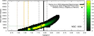
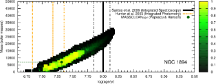
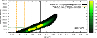
Figure 10: Output from MASSCLEANage: finding probabilistic regions in the mass - age plane, based on observed UBV magnitudes for these clusters. These diagrams show the very strong correlation between cluster mass and age in integrated UBV colors. Our best solution for NGC 1894 does not match the age given by Santos et al. 2006.

3.2 Further Tests of the MASSCLEANage Program

Regrettably, the Santos et al. 2006 study has only a small overlap with the Hunter et al. 2003 catalog of clusters, a consistent, high quality UBV dataset with SSP derived ages. But we wish to provide a further test of the MASSCLEANage package. The Hunter et al. 2003 study includes over 900 LMC clusters, but only a fraction of those clusters are good examples. By this we mean, their location in the color-color diagram allows them to be more clearly aged using SSP models.

We selected a subset of 30 clusters, which cover a wide range of $(U-B)_{0}$ and $(B-V)_{0}$ colors, but are also located close to the infinite mass limit (see the yellow triangles in Figure 8). The selected clusters are given in Table 2. Due to their locations in the color-color diagram, the age determination based on the classical $\chi^{2}$ minimization methods and infinite mass limit is expected to be relatively accurate (e.g. Lançon & Mouhcine 2000; Popescu & Hanson 2010a). As shown in Figure 11, our MASSCLEANage results are in good agreement with the ages from Hunter et al. 2003 based on SSP model fits. However, we can also derive the mass, and this is presented in column 8 of the Table 2. New values for age and mass for all the clusters with $UBV$ colors in the Hunter et al. 2003 catalog and derived using MASSCLEANage will be presented in a subsequent paper (Popescu et al.  2010, in preparation).

Figure 11: We have further checked the consistency of the ages derived using MASSCLEANages by selecting a subset of Hunter et al. 2003 clusters with previously well constrained ages. These data are also shown in Table 2.

Table 2: Results

	Integrated Photometry (Hunter et al. 2003)					MASSCLEAN
Name	$M_{V}$	$(U-B)_{0}$	$(B-V)_{0}$	Age		Age	Age	Mass
	$(mag)$	$(mag)$	$(mag)$	$(Myr)$		$(Myr)$	$(log)$	$(M_{\sun}$)
$1$	$2$	$3$	$4$	$5$		$6$	$7$	$8$
KMK 88-88	$-7.848$	$-0.768$	$0.076$	$15.7$		$15.85^{+3.65\phantom{0}}_{-2.36}\phantom{0}$	$7.20^{+0.09}_{-0.07}$	$7,000^{+3,000\phantom{0}}_{-3,000}$
H 88-308	$-7.151$	$-0.716$	$0.265$	$13.6$		$16.22^{+5.66\phantom{0}}_{-3.33}\phantom{0}$	$7.21^{+0.13}_{-0.10}$	$3,000^{+2,000\phantom{0}}_{-500}$
NGC 2009	$-8.047$	$-0.735$	$0.204$	$12.6$		$16.22^{+2.84\phantom{0}}_{-4.74}\phantom{0}$	$7.21^{+0.07}_{-0.15}$	$8,000^{+2,000\phantom{0}}_{-5,000}$
SL 288	$-6.897$	$-0.562$	$-0.097$	$19.1$		$18.62^{+8.92\phantom{0}}_{-5.44}\phantom{0}$	$7.27^{+0.17}_{-0.15}$	$1,500^{+2,500\phantom{0}}_{-1,300}$
NGC 1922	$-7.742$	$-0.631$	$0.027$	$23.9$		$20.42^{+7.77\phantom{0}}_{-2.22}\phantom{0}$	$7.31^{+0.14}_{-0.05}$	$6,000^{+5,000\phantom{0}}_{-2,000}$
BSDL 1181	$-6.150$	$-0.203$	$0.050$	$31.3$		$37.15^{+21.73}_{-8.97}\phantom{0}$	$7.57^{+0.20}_{-0.12}$	$1,000^{+1,000\phantom{0}}_{-300}$
SL 423	$-6.305$	$-0.442$	$0.071$	$43.3$		$51.29^{+11.81}_{-11.47}\phantom{0}$	$7.71^{+0.09}_{-0.11}$	$3,000^{+2,000\phantom{0}}_{-1,000}$
HS 371	$-6.409$	$-0.292$	$0.166$	$105.8$		$100.00^{+23.03}_{-36.90}\phantom{0}$	$8.00^{+0.09}_{-0.20}$	$5,000^{+2,000\phantom{0}}_{-2,000}$
KMK 88-45	$-5.116$	$-0.338$	$0.208$	$92.2$		$109.65^{+10.58}_{-43.58}\phantom{0}$	$8.04^{+0.04}_{-0.22}$	$2,000^{+500}_{-1,300\phantom{0}}$
HS 318	$-4.462$	$-0.267$	$0.172$	$112.8$		$109.65^{+38.26}_{-14.15}\phantom{0}$	$8.04^{+0.13}_{-0.06}$	$700^{+800\phantom{0}\phantom{.}\phantom{0}}_{-200}$
SL 408A	$-4.086$	$-0.277$	$0.208$	$111.0$		$128.82^{+49.00}_{-28.82}\phantom{0}$	$8.11^{+0.14}_{-0.11}$	$700^{+300\phantom{0}\phantom{.}\phantom{0}}_{-400}$
HS 346	$-6.119$	$-0.228$	$0.211$	$153.9$		$147.91^{+18.05}_{-52.41}\phantom{0}$	$8.17^{+0.05}_{-0.19}$	$5,000^{+1,000\phantom{0}}_{-2,000}$
KMK 88-76	$-4.673$	$-0.216$	$0.246$	$162.2$		$158.49^{+41.04}_{-46.29}\phantom{0}$	$8.20^{+0.10}_{-0.15}$	$1,500^{+500\phantom{0}\phantom{.}\phantom{0}}_{-800}$
NGC 1695	$-6.845$	$-0.231$	$0.167$	$144.0$		$162.18^{+46.75}_{-52.53}\phantom{0}$	$8.21^{+0.11}_{-0.17}$	$11,000^{+4,000\phantom{0}}_{-3,000}$
KMHK 494	$-4.378$	$-0.148$	$0.245$	$178.0$		$177.83^{+62.05}_{-46.00}\phantom{0}$	$8.25^{+0.13}_{-0.13}$	$1,000^{+500\phantom{0}\phantom{.}\phantom{0}}_{-300}$
SL 110	$-5.334$	$-0.195$	$0.169$	$184.8$		$186.21^{+62.05}_{-46.00}\phantom{0}$	$8.27^{+0.07}_{-0.14}$	$3,000^{+1,000\phantom{0}}_{-1,000}$
HS 218	$-5.607$	$-0.183$	$0.213$	$195.4$		$199.53^{+14.27}_{-41.04}\phantom{0}$	$8.30^{+0.03}_{-0.10}$	$4,000^{+1,000\phantom{0}}_{-1,000}$
KMK 88-49	$-4.496$	$-0.160$	$0.198$	$210.8$		$208.93^{+14.27}_{-41.04}\phantom{0}$	$8.32^{+0.05}_{-0.11}$	$1,500^{+500\phantom{0}\phantom{.}\phantom{0}}_{-500}$
KMK 88-35	$-4.488$	$-0.155$	$0.228$	$221.1$		$208.93^{+30.95}_{-26.96}\phantom{0}$	$8.32^{+0.06}_{-0.06}$	$1,500^{+500\phantom{0}\phantom{.}\phantom{0}}_{-500}$
SL 160	$-5.077$	$-0.132$	$0.173$	$240.9$		$245.47^{+23.68}_{-21.60}\phantom{0}$	$8.39^{+0.04}_{-0.04}$	$3,000^{+500\phantom{0}\phantom{.}\phantom{0}}_{-500}$
SL 580	$-4.957$	$-0.097$	$0.165$	$272.3$		$281.84^{+72.97}_{-63.06}\phantom{0}$	$8.45^{+0.10}_{-0.11}$	$3,000^{+1,000\phantom{0}}_{-1,000}$
SL 224	$-5.489$	$-0.072$	$0.191$	$303.5$		$302.00^{+52.81}_{-50.80}\phantom{0}$	$8.48^{+0.07}_{-0.08}$	$5,000^{+1,000\phantom{0}}_{-1,000}$
H 88-17	$-3.290$	$-0.051$	$0.209$	$335.1$		$331.13^{+49.06}_{-61.98}\phantom{0}$	$8.52^{+0.06}_{-0.09}$	$700^{+300\phantom{0}\phantom{.}\phantom{0}}_{-200}$
HS 32	$-3.984$	$-0.044$	$0.172$	$319.3$		$354.81^{+43.29}_{-66.41}\phantom{0}$	$8.55^{+0.05}_{-0.09}$	$1,500^{+250\phantom{0}\phantom{.}\phantom{0}}_{-500}$
H 88-235	$-4.046$	$-0.029$	$0.218$	$356.7$		$363.08^{+35.03}_{-74.67}\phantom{0}$	$8.56^{+0.04}_{-0.10}$	$1,500^{+500\phantom{0}\phantom{.}\phantom{0}}_{-500}$
HS 76	$-4.331$	$0.010$	$0.272$	$411.6$		$389.05^{+112.14}_{-72.81}$	$8.59^{+0.11}_{-0.09}$	$2,000^{+500\phantom{0}\phantom{.}\phantom{0}}_{-500}$
H 88-59	$-3.965$	$-0.008$	$0.258$	$377.6$		$389.05^{+78.69}_{-65.45}\phantom{0}$	$8.59^{+0.08}_{-0.08}$	$1,500^{+500\phantom{0}\phantom{.}\phantom{0}}_{-500}$
SL 588	$-5.436$	$0.095$	$0.303$	$609.0$		$602.56^{+156.02}_{-166.04}$	$8.78^{+0.10}_{-0.14}$	$8,000^{+2,000\phantom{0}}_{-3,000}$
HS 338	$-4.338$	$0.109$	$0.308$	$633.1$		$630.96^{+127.62}_{-152.33}$	$8.80^{+0.08}_{-0.12}$	$3,000^{+1,000\phantom{0}}_{-1,000}$
SL 268	$-7.032$	$0.181$	$0.596$	$1,000.0$		$1,148.15^{+110.77}_{-256.90}$	$9.06^{+0.04}_{-0.11}$	$50,000^{+5,000}_{-10,000}$

4 Discussion & Conclusions

That there would be degeneracies in the UBV color-color diagrams affecting the derivation of age as shown in Figures 7 and 8, was previously recognized by many (e.g. Bruzual & Charlot 2003; Cerviño & Valls-Gabaud 2009; Buzzoni 1989; Chiosi 1989; Bruzual 2002; Bruzual 2010; Cerviño & Luridiana 2004; Cerviño & Luridiana 2006; Fagiolini et al. 2007; Lançon & Mouhcine 2000; Lançon & Fouesneau 2009; Fouesneau & Lançon 2009; Fouesneau & Lançon 2010; González et al. 2004; González-Lópezlira et al. 2005; González-Lópezlira et al. 2010; Maíz Apellániz 2009; Pandey et al. 2010; Popescu & Hanson 2010a). However, the scatter experienced in the integrated magnitude of a cluster also means using luminosity as a proxy for mass is highly dangerous for clusters of moderate and low mass. This is clearly demonstrated in our simulations, particularly in Figure 4. Present day SSP models are not designed to work with moderate and low mass clusters (e.g. Bruzual 2002; Bruzual 2010; Lançon & Mouhcine 2000; Popescu & Hanson 2009; Popescu & Hanson 2010a). Yet, this is in fact the way in which mass functions for stellar clusters in other galaxies have been derived. For some studies, it might be argued the masses are high enough that the errors are not extreme (Larsen & Richtler 2000), but this method is being extended to a lower mass regime such as in the LMC (e.g. Billettt et al. 2002; Hunter et al. 2003), simply because there was no other way to derive this critical information.

The MASSCLEANcolors database is sufficiently populated now so it can be used to work back and derive mass and age for moderate and lower mass clusters in the LMC with a known (correctable) extinction. To make this possible with just three input bands, the dataset uses the Padova 2008 models (Marigo et al. 2008) with a metallicity of $Z=0.008$ ([Fe/H]=-0.6). While the simulations created for the database extend to ages up to $log(age/yr)=9.5$, we have avoided applying the current inference package MASSCLEANage on clusters in the LMC for which previous indicators suggested ages greater than $log(age/yr)>9.0$. This is because of our concern in the evolutionary models at such age and the inevitable drop in metallicity for the very oldest LMC clusters. It seems simplistic to assume the same metallicity can be applied to old clusters as to recently formed clusters, however, the metallicity of the LMC does appears to have been reasonably slow changing over a fairly long period of time, from relatively recent times until about $log(age/yr)=9.5$ (Bica et al. 1998; Harris & Zaritsky 2009; Piatti et al. 2009). These studies also show that for some young clusters, $log(age/yr)<8$, the adopted metallicity for the current MASSCLEANcolors database may be too low by a few dex. Whether the MASSCLEANcolors database might be extended to include LMC clusters over a broader range of metallicities, from [Fe/H] = -1 to 0 and for $log(age/yr)>9.5$, and if this might prove significant in deriving accurate age and mass estimates remains to be explored. If such an additional parameter would be added to the database, more input photometry will be needed for the stellar cluster in question, to keep the search from becoming hopelessly degenerate over all the properties.

References

- (1)
- Bica et al. (1998) Bica, E., Geisler, D., Dottori, H., Claria, J.H., Piatti, A.E. Santos, J.F. 1998, AJ, 116, 723
- Billett et al. (2002) Billett, O. H., Hunter, D. A., Elmegreen, B. G. 2002, AJ, 123, 1454
- Brocato et al. (1999) Brocato, E., Castellani, V., Raimondo, G., Romaniello, M. 1999, A&AS, 136, 65
- Brocato et al. (2000) Brocato, E., Castellani, V., Poli, F. M., Raimondo, G. 2000, A&AS, 146, 91
- Bruzual (2002) Bruzual, G. 2002, IAUS 207, 616
- Bruzual (2010) Bruzual A., G. 2010, RSPTA, 368, 783
- Bruzual & Charlot (2003) Bruzual, G. & Charlot, S. 2003, MNRAS, 344, 1000
- Buzzoni (1989) Buzzoni, A. 1989, ApJS, 71, 817
- Cantiello et al. (2003) Cantiello, M., Raimondo, G., Brocato, E., Capaccioli, M. 2003, AJ, 125, 2783
- Cerviño & Luridiana (2004) Cerviño, M. & Luridiana, V., 2004, A&A, 413, 145
- Cerviño & Luridiana (2006) Cerviño, M. & Luridiana, V., 2006, A&A, 451, 475
- Cerviño & Valls-Gabaud (2003) Cerviño, M. & Valls-Gabaud, D., 2003, MNRAS, 338, 481
- Cerviño & Valls-Gabaud (2009) Cerviño, M. & Valls-Gabaud, D., 2009, Ap&SS, 324, 91
- Chandar et al. (2010a) Chandar, R., Fall, S.M, Whitmore, B.C. 2010a, ApJ, 711, 1263
- Chandar et al. (2010b) Chandar, R., Whitmore, B.C., Fall, S.M. 2010b, ApJ, 713, 1343
- Chiosi (1989) Chiosi, C. 1989, RMxAA, 18, 125
- Fagiolini et al. (2007) Fagiolini, M., Raimondo, G., Degl’Innocenti, S. 2007 A&A, 462, 107
- Fouesneau & Lançon (2009) Fouesneau, M. & Lançon, A. 2009, preprint - astro-ph/0908.2742
- Fouesneau & Lançon (2010) Fouesneau, M. & Lançon, A. 2010, preprint - astro-ph/1003.2334
- Girardi et al. (1995) Girardi, L., Bressan, A., Chiosi, C., Bertelli, G., Nasi, E. 1995 A&A, 298, 87
- González et al. (2004) González, R.A., Liu, M.C., Bruzual A., G. 2004, ApJ, 611, 270
- González-Lópezlira et al. (2005) González-Lópezlira, R.A., Albarrán, M.Y., Mouhcine, M., Liu, M.C., Bruzual-A., G., de Batz, B. 2005, MNRAS, 363, 1279
- González-Lópezlira et al. (2010) González-Lópezlira, R.A., Bruzual-A., G., Charlot, S., Ballesteros-Paredes, J., Loinard, L. 2010, MNRAS, preprint - astro-ph/0908.4133
- Hancock et al. (2008) Hancock, M., Smith, B.J., Giroux, M.L., Struck, C. 2008, MNRAS 389, 1470
- Harris & Zaritsky (2009) Harris, J. & Zaritsky, D. 2009, AJ, 138, 1243
- Hunter et al. (2003) Hunter, D.A., Elmegreen, B.G., Dupuy, T.J., Mortonson, M. 2003, AJ, 126, 1836
- Kroupa (2002) Kroupa, P. 2002, Sci, 295, 82
- Lamers et al. (2005) Lamers, H. J. G. L. M., Gieles, M., Bastian, N., Baumgardt, H., Kharchenko, N. V., Portegies Zwart, S. 2005, A&A, 441, 117
- Lançon & Mouhcine (2000) Lançon, A. & Mouhcine, M. 2000, ASPC, 211, 34
- Lançon & Mouhcine (2002) Lançon, A. & Mouhcine, M. 2002, A&A, 393, 167
- Lançon & Fouesneau (2009) Lançon, A. & Fouesneau, M. 2009, ASPC, preprint - astro-ph/0903.4557
- Larsen & Richtler (2000) Larsen, S. S. & Richtler, T. 2000, A&A, 354, 836
- Larsen (2009) Larsen, S.S. 2009, A&A, 494, 539
- Lejeune & Schaerer (2001) Lejeune, T. & Schaerer, D. 2001, A&A, 366, 538
- Maíz Apellániz (2009) Maíz Apellániz, J. 2009, ApJ, 699, 1938
- Marigo et al. (2008) Marigo, P., Girardi, L., Bressan, A., Groenewegen, M. A. T., Silva, L., Granato, G. L. 2008, A&A, 482, 833
- Mora et al. (2009) Mora, M.D. Larsen, S.S., Kissler-Patig, M., Brodie, J.O., Richtler, T. 2009 A&A, 501, 949
- Pandey et al. (2010) Pandey, A.K., Sandhu, T.S., Sagar, R., & Battinelli, P. 2010, MNRAS, 403, 1491
- Pessev et al. (2009) Pessev, P. M., Goudfrooij, P., Puzia, T. H., Chandar, R. 2008, MNRAS, 385, 1535
- Piatti et al. (2009) Piatti, A.E., Geisler, D., Sarajedini, A., Gallart, C. 2009, A&A, 501, 585
- Popescu & Hanson (2009) Popescu, B. & Hanson, M.M. 2009, AJ, 138, 1724
- Popescu & Hanson (2010a) Popescu, B. & Hanson, M.M. 2010a,ApJ, 713, L21
- Popescu & Hanson (2010b) Popescu, B. & Hanson, M.M. 2010b, Proceedings International Astronomical Union Symposium No. 266, p. 511, Star Clusters - Basic Galactic Building Blocks throughout Time and Space, Editors: Richard de Grijs & Jacques R. D. Lepine
- Raimondo et al. (2005) Raimondo, G., Brocato, E., Cantiello, M., Capaccioli, M. 2005, AJ, 130, 2625
- Raimondo (2009) Raimondo, G. 2009, ApJ, 700, 1247
- Santos & Frogel (1997) Santos, J.F.C. & Frogel, J.A. 1997, ApJ, 479, 764
- Santos et al. (2006) Santos, J.F.C, Clariá, J.J., Ahumada, A.V., Bica, E., Piatti, A.E., Parisi, M.C. 2006, A&A, 448, 1023
- Searle et al. (1980) Searle, L., Wilkinson, A., Bagnuolo, W.G. 1980, ApJ, 239, 803
- van den Bergh (1981) van den Bergh, S. 1981, A&AS, 46, 79