Bulk and surface energetics of lithium hydride crystal:
benchmarks from quantum Monte Carlo and quantum chemistry

Abstract

We show how accurate benchmark values of the surface formation energy of crystalline lithium hydride can be computed by the complementary techniques of quantum Monte Carlo (QMC) and wavefunction-based molecular quantum chemistry. To demonstrate the high accuracy of the QMC techniques, we present a detailed study of the energetics of the bulk LiH crystal, using both pseudopotential and all-electron approaches. We show that the equilibrium lattice parameter agrees with experiment to within $0.03~{}$%, which is around the experimental uncertainty, and the cohesive energy agrees to within around $10$ meV per formula unit. QMC in periodic slab geometry is used to compute the formation energy of the LiH (001) surface, and we show that the value can be accurately converged with respect to slab thickness and other technical parameters. The quantum chemistry calculations build on the recently developed hierarchical scheme for computing the correlation energy of a crystal to high precision. We show that the hierarchical scheme allows the accurate calculation of the surface formation energy, and we present results that are well converged with respect to basis set and with respect to the level of correlation treatment. The QMC and hierarchical results for the surface formation energy agree to within about $1$ %.

I Introduction

The surface formation energies of materials are key quantities in fields as diverse as nanotechnology, mineral science and fracture mechanics. However, the accurate measurement of surface energies is fraught with difficulties, so there is often a need to rely on calculated values. In principle, electronic-structure methods based on density-functional theory (DFT) should be capable of giving reliable surface energies, but in practice it is found that computed values depend strongly on the approximation used for the exchange-correlation energy. goniakowski96 ; mattsson_computing_2002 ; yu_first-principles_2004 ; binnie_benchmarking_2009 There are two main kinds of electronic-structure technique that allow one to go beyond DFT and achieve better accuracy: quantum Monte Carlo (QMC), and the wavefunction-based correlation techniques usually associated with molecular quantum chemistry (QC). We show here how these two very different approaches can be used in a complementary way to produce accurate benchmark values for surface formation energy, using as a test case the (001) surface of crystalline LiH.

There have been many DFT calculations of the surface formation energies $\sigma$ of different kinds of materials, including ionic compounds, covalent semiconductors and metals. In some cases, the variation of predicted $\sigma$ values with the assumed exchange-correlation functional has been studied, and it is found that generalized gradient approximations (GGA) such as PBE and PW91 often give $\sigma$ values that are $\sim 30$ % lower than those predicted by the local density approximation (LDA).binnie_benchmarking_2009 ; alf_energetics_2006 ; yu_first-principles_2004 ; mattsson_computing_2002 Since GGAs are generally more accurate than LDA for bonding energies, and since the energy needed to form a surface would seem to be closely related to the energy needed to break bonds, it might be expected that GGA values of $\sigma$ would be more accurate. However, in the few cases where there are reliable experimental data, this expectation is not fulfilled, and the rather scattered evidence suggests that the LDA may be more accurate.alf_energetics_2006 ; yu_first-principles_2004 ; mattsson_computing_2002 A connection has been made with the superiority of LDA over GGAs for the surface energy of jellium.almeida_surface_2002

In this rather confused situation, it is helpful to seek ways of computing benchmark values of $\sigma$ which do not suffer from the uncertainties of DFT. Quantum Monte Carlo, and specifically diffusion Monte Carlo (DMC) foulkes_quantum_2001 ; needs_continuum_2010 offers one way of achieving this. It is well established that DMC is usually much more accurate than DFT for the energetics of extended systems, and there are ways of systematically improving its accuracy. Nevertheless, it is subject to errors that are not completely controllable, and this is where the methods of molecular quantum chemistry can play an important role. The electron-correlation techniques that we use here are mainly second-order Møller-Plesset theory (MP2) and the coupled-cluster scheme CCSD(T) (including single, double and a perturbative treatment of triple excitations). Efforts to apply these QC techniques to the energetics of extended systems go back many years, particularly using the so-called incremental approach stoll92 ; paulus_method_2006 . More recently, the MP2 approximation has been implemented for periodic systems in several codes kresse_mp2 ; pisani08 . The present authors have reported a technique referred to as the hierarchical method for applying molecular QC methods to perfect crystals, and for the case of LiH have shown that it can deliver the cohesive energy to an absolute accuracy of $\sim 5$ meV per formula unit and the equilibrium lattice parameter to better than $0.1$ %.nolan_calculation_2009 ; manby_extension_2006

We have chosen to study the surface energetics of LiH, partly because it is a material for which we expect DMC to give very high accuracy, and partly because we already know that hierarchical QC is very accurate. nolan_calculation_2009 The crystal has the rock–salt structure, and the simplicity of this structure facilitates the calculations. We have several main aims. First, we want to show that DMC does indeed deliver high accuracy for the properties of the LiH crystal, particularly if we use all-electron rather than pseudopotential DMC (pp-DMC). Second, we report our periodic slab calculations of $\sigma$ for the LiH (001) surface, using both pseudopotential and all-electron DMC, and we show that we can achieve a high degree of convergence with respect to slab thickness and other technical parameters. Third, we show that the hierarchical QC scheme that gives such good accuracy for bulk LiH also provides a practical way of obtaining benchmark values of $\sigma$. The hierarchical methods allow us to calculate explicitly the contribution of core-valence correlation to $\sigma$, and we shall see that this is significant. Naturally, close agreement between the $\sigma$ values computed by the QMC and QC approaches supports the credibility of both, and this will be carefully assessed.

II Techniques

II.1 Quantum Monte Carlo

For present purposes, the name quantum Monte Carlo refers to two techniques for determining the ground-state energy of a many-electron system (for reviews, see e.g. Refs. foulkes_quantum_2001 ; needs_continuum_2010 ). Our high-precision results are obtained using diffusion Monte Carlo (DMC), a technique that projects out the ground state by evolving the many-electron wavefunction in imaginary time with the aid of an approximate trial wavefunction. An optimized form of this trial function is computed using variational Monte Carlo (VMC), which is an implementation of the variational principle of quantum mechanics. The VMC and DMC calculations in this work are performed using the CASINO package needs_continuum_2010 .

The trial wavefunctions used here have the standard single-determinant Slater-Jastrow form:

$$\Psi_{\rm T}=D_{\uparrow}D_{\downarrow}e^{J}\;,$$ (1)

where $D_{\uparrow}$ and $D_{\downarrow}$ are up- and down-spin Slater determinants of single-electron orbitals $\psi_{n}$. Electron correlation is approximately described by $J$, which is a sum of three types of terms: electron-electron terms $u$, electron-nucleus terms $\chi$, and electron-electron-nucleus terms $f$. These three terms contain parameters that are optimized using VMC, so as to make $\Psi_{\rm T}$ as close as possible to the true ground-state wavefunction. The optimization works with the local energy $E_{\rm L}\equiv\Psi_{\rm T}^{-1}\hat{H}\Psi_{\rm T}$, where $\hat{H}$ is the many-electron Hamiltonian. We follow the common procedure of varying the parameters so as to minimize the variance of $E_{\rm L}$ (the variance would be zero if $\Psi_{\rm T}$ were the exact ground-state wavefunction). VMC can be used equally well as an all-electron technique or with non-local pseudopotentials to represent the interaction between valence electrons and atomic cores.

The idea of DMC ceperley_ground_1980 ; foulkes_quantum_2001 ; needs_continuum_2010 is to represent the exact many-electron wavefunction $\Phi$ as a density of brownian particles, or ‘walkers’. In the evolution of the wavefunction according to the time-dependent Schrödinger equation in imaginary time, the optimized approximation $\Psi_{\rm T}$ from VMC is used to guide the walkers, in a manner related to importance sampling. DMC aims to stochastically simulate the diffusion, birth, death and drift of the walkers, which, after an equilibration period, samples the exact ground-state wavefunction. In practice, the fermionic nature of electrons prevents DMC from being completely exact, and the nodal surfaces of the wavefunction are constrained to be those of $\Psi_{\rm T}$ – this is the well-known fixed-node approximation anderson75 . We shall see that this approximation incurs only small errors in the present work. A number of other technical issues have to be addressed, including time-step errors, pseudopotential errors, the choice and representation of the single-electron orbitals $\psi_{n}$, and the stability of walker populations, and we summarize these next. The treatment of system size errors will be discussed in Sec. II.2.

The walkers propagate by using the approximate small-time-step Green’s function as a transition probability in configuration space. The approximate Green’s function also includes a term that gives a probability for a given walker to ‘branch’ (become two walkers) or to be discarded entirely. The use of a discrete time-step incurs errors, but these can be rendered negligible by the usual procedure of extrapolating to the zero-time-step limit. We shall present both pseudopotential and all-electron DMC calculations on the LiH bulk and surface. For the pseudopotential work, we use the Dirac-Fock pseudopotentials due to Trail and Needs trail_smooth_2005 ; trail_norm-conserving_2005 . It is difficult to treat non-local pseudopotentials in DMC, and we employ the usual locality approximation mitas_nonlocal_1991 , which introduces errors proportional to the square of the difference between $\Psi_{\rm T}$ and the exact ground-state wavefunction $\Phi$. The comparison of our pseudopotential and all-electron results will help us to quantify these errors.

The single-electron orbitals $\psi_{n}$ used in the trial wavefunction $\Psi_{\rm T}$ (see Eq. (1)) were generated by DFT calculations with the LDA functional. We make this choice because there is considerable evidence kent1998 ; ma2009 that this gives a $\Psi_{\rm T}$ that is closer to the true ground state. The $\psi_{n}$ were computed by plane-wave calculations with the quantum espresso package QE-2009 . However, the direct use of $\psi_{n}$ in a plane-wave representation in DMC is very inefficient, and instead we re-expand the $\psi_{n}$ in a blip-function (B-spline) basis alf_efficient_2004 , using the standard relation between the blip-grid spacing and the plane-wave cut-off. In the case of all-electron DMC, a further modification is necessary, since it is crucially important that $\Psi_{\rm T}$ has the correct electron-nuclear cusp at the nuclear positions. The technique we have used to ensure this with the blip basis is described in Appendix A.

Since walkers can branch or be discarded after each step, the walker population fluctuates. A reference energy in the approximate Green’s function allows us to bias the branching, and thus control the population. However, in regions of particularly low energy (especially divergences at point charges), this mechanism is not enough, and a walker trapped in this region (and its offspring) can branch repeatedly, causing a population explosion which destroys the statistics of subsequent moves.

II.2 QMC for bulk and surface energies

Correction for errors due to the limited size of the periodically repeated cell is important in the calculation of both bulk and surface energies. As usual, we distinguish between single-particle and many-body errors. The former are due to the fact that $k$-point sampling cannot be performed with DMC, and are analogous to those that would arise in single-particle methods such as DFT without $k$-point samplng; the latter are due to the spurious interaction of electrons with their periodic images. To correct for single-particle errors, we use the formula foulkes_quantum_2001 :

$$E_{\infty}=E_{\rm cell}^{\rm DMC}+a(E_{\infty}^{\rm DFT}-E_{\rm cell}^{\rm DFT})\;,$$ (2)

where $E_{\rm cell}^{\rm DMC}$ and $E_{\rm cell}^{\rm DFT}$ are the energies of the given cell with DMC and DFT (no $k$-point sampling with DFT), $E_{\infty}^{\rm DFT}$ is the DFT energy of the cell with perfect $k$-point sampling, and $E_{\infty}$ is the corrected DMC energy; if enough data for different system sizes are available, $a$ can be treated as a fitting parameter.

One way of correcting for many-body size errors is to use a modified form of the Coulomb interaction known as the Model Periodic Coulomb (MPC) interaction in the DMC calculations. fraser_finite-size_1996 ; williamson_elimination_1997 ; kent_finite-size_1999 We used this technique, in combination with Eq. (2) for our all-electron calculations on bulk LiH. An alternative approach is the scheme due to Kwee et al. kwee_finite-size_2008 , which corrects for both single–particle and many–body errors in a single formula:

$$E_{\infty}=E_{N}^{\rm DMC}+E_{\infty}^{\rm LDA}-E_{N}^{\rm KZK}\;,$$ (3)

which somewhat resembles Eq. (2). Here, $E_{\rm cell}^{\rm KZK}$ is a DFT-like energy of the cell (no $k$-point sampling), which uses a functional designed to mimic the sum of single-particle and many-body errors, while $E_{\infty}^{\rm LDA}$ is the same as $E_{\infty}^{\rm DFT}$ in Eq. (2), evaluated with the LDA functional. We used this scheme of Kwee et al. for the pseudopotential calculations on the bulk. Whichever method is used to correct for the many-body size errors, in the case of the bulk calculations we apply a further two-point extrapolation to remove residual finite-size errors. This extrapolation employs the formula:

$$E_{\infty}=\left(NE_{N}-ME_{M}\right)\left/\left(N-M\right)\right.\;,$$ (4)

where $E_{N}$ and $E_{M}$ are the DMC energies per formula unit of supercells containing $N$ and $M$ formula units respectively.ceperley_ground_1980 ; ceperley_ground_1987 ; rajagopal_variational_1995 ; zong_spin_2002

Our DMC calculations of the surface formation energy are performed in slab geometry, so that we work with slabs having infinite extent in the plane of the surface and having a specified number $N$ of ionic layers. Periodic boundary conditions are applied in the surface plane, so that we have supercell geometry only in two dimensions. With the blip basis set used for the present work, it is unnecessary to apply periodic boundary conditions in the direction perpendicular to the surface.

As usual, the surface formation energy $\sigma$ is the work needed to create an area $A$ of new surface, starting from the perfect bulk crystal, divided by $A$. In slab geometry, if $E_{\rm slab}(N)$ is the energy per supercell of the $N$-layer slab, $\nu_{\rm slab}(N)$ is the number of formula units per supercell of the $N$-layer slab, and $e_{\rm bulk}$ is the energy per formula unit of the bulk crystal, then $\sigma$ is given by:

$$\sigma=\lim\left(E_{\rm slab}(N)-\nu_{\rm slab}(N)e_{\rm bulk}\right)/A\;,$$ (5)

where $A$ is the total surface area (both faces) per supercell of the slab. In Eq. (5), we must take the limit as the number of layers $N$ and the surface dimensions of the supercell both tend to infinity. For comparison with experimental data, the ionic positions in the slab should also be relaxed to equilibrium, but in the present work we are concerned mainly with comparing different theoretical approaches, and we focus on the unrelaxed value of $\sigma$, for which all ions in the slab have their bulk positions.

Instead of using Eq. (5) directly, we prefer to use the well-known procedure of extracting $\sigma$ from a series of slab calculations of increasing $N$, using the fact that as $N\rightarrow\infty$, $E_{\rm slab}$ has the asymptotic form:

$$E_{\rm slab}(N)\rightarrow A\sigma+NE_{\rm layer}\;.$$ (6)

Here, $\sigma$ is the surface formation energy with the chosen surface supercell, and $E_{\rm layer}$ is the bulk energy per ionic layer with this supercell. Eq. (6) is equivalent to Eq. (5), but the extraction of $\sigma$ for a given surface supercell from Eq. (6) is usually more robust. We note that the value of $E_{\rm layer}$ can be cross–checked against independent calculations on the bulk crystal, since $NE_{\rm layer}/\nu_{\rm slab}(N)$ should be very close to $e_{\rm bulk}$.

When correcting for finite–size errors in slab geometry, compensation for many–body errors poses technical problems, and we therefore used only the single–particle correction of Eq. (2).

II.3 Correlated quantum chemistry

We show here how the hierarchical method manby_extension_2006 ; nolan_calculation_2009 , originally developed to treat bulk crystals, can be used to calculate surface formation energy. We recall that the hierarchical method begins by separating the total energy $e^{\rm tot}$ per primitive cell of a crystal into Hartree-Fock and correlation parts:

$$e^{\rm tot}=e^{\rm HF}+e^{\rm corr}\;.$$ (7)

The correlation energy $e^{\rm corr}$ is further separated into a molecular contribution and the so-called “correlation residual”:

$$e^{\rm corr}=e_{\rm mol}^{\rm corr}+\Delta e^{\rm corr}\;.$$ (8)

In the case of a compound AB having the rock-salt structure, $e_{\rm mol}^{\rm corr}$ is the correlation contribution to the binding energy of the AB molecule, with the bond length taken equal to the nearest-neighbour distance in the crystal.

The hierarchical method works by combining energies of a sequence of finite clusters manby_extension_2006 ; nolan_calculation_2009 in such a way as to eliminate surface effects. For the rock-salt structure, we take cuboidal clusters having $l$, $m$ and $n$ ions along the three perpendicular edges. By conventional quantum chemistry techniques, we can compute accurately the total energy $E_{lmn}^{\rm tot}$ of each $l\times m\times n$ cluster, which is then decomposed into Hartree-Fock, molecular and residual parts:

$$E_{lmn}^{\rm tot}=E_{lmn}^{\rm HF}+\frac{1}{2}lmn\,e_{\rm mol}^{\rm corr}+\Delta E_{lmn}^{\rm corr}\;.$$ (9)

The total energy per primitive cell in the infinite crystal is then:

$$e^{\rm tot}=\lim_{l,m,n\rightarrow\infty}\frac{2}{lmn}E_{lmn}^{\rm tot}=e^{\rm HF}+e_{\rm mol}^{\rm corr}+\lim_{l,m,n\rightarrow\infty}\frac{2}{lmn}\Delta E_{lmn}^{\rm corr}\;.$$ (10)

We calculate the Hartree-Fock contribution $e^{\rm HF}$ using standard periodic codes, and $e_{\rm mol}^{\rm corr}$ is obtained by conventional quantum chemistry techniques. To perform the limiting process in the third term on the right, the hierarchical method expresses $\Delta E_{lmn}^{\rm corr}$ as:

$$\Delta E_{lmn}^{\rm corr} = 8E^{000}+4[(l-2)+(m-2)+(n-2)]E^{001}$$ (11)

$$+ 2[(m-2)(n-2)+(n-2)(l-2)+(l-2)(m-2)]E^{011}$$

$$+ (l-2)(m-2)(n-2)E^{111}\;,$$

where the coefficients $E^{000}$, $E^{001}$, $E^{011}$ and $E^{111}$ represent the energies of corner, edge, face and bulk sites, respectively. [Note that the definitions of $E^{011}$, $E^{001}$ and $E^{000}$ are affected by our decision to use factors $(l-2)(m-2)(n-2)$, $(m-2)(n-2)$, etc, rather than $lmn$, $mn$, etc. The reason for making this particular choice of factors is discussed in Ref. nolan_calculation_2009 .]

Our procedure for obtaining the values of the coefficients in the limit of infinite $l$, $m$, $n$ requires us to extract $E^{000}$, $E^{001}$, $E^{011}$ and $E^{111}$ from sets of four independent clusters, and then systematically to increase the size of the clusters in these sets, as described in detail in Ref. nolan_calculation_2009, . For the cohesive energy, only the limiting value of $E^{111}$ is needed, since $\Delta e^{\rm corr}=2E^{111}$. However, the procedure also yields the limiting values of $E^{011}$, $E^{001}$ and $E^{000}$. The value of $E^{011}$ can be used to obtain the value of the unrelaxed surface formation energy $\sigma$.

The coefficient $E^{111}$ is the contribution to the energy of a large cluster from an atom in the interior; $E^{011}$ is the same for an atom on the surface. When a surface is formed by opening a gap in the crystal, each atom in the newly formed surface contributes $E^{011}-E^{111}$ to the energy difference. The area of the surface occupied by each atom is $a^{2}/2$, so the correlation contribution to the formation energy of a new surface is $2(E^{011}-E^{111})/a^{2}$ per ion. We therefore obtain

$$\sigma=\sigma^{\rm HF}+4(E^{011}-E^{111})/a^{2}\;.$$ (12)

We compute the Hartree-Fock part $\sigma^{\rm HF}$ using standard periodic codes (details will be given later).

II.4 Zero-point corrections

Both quantum Monte Carlo and quantum chemistry techniques employ static calculations, and ignore zero-point energies. In this work, in order to facilitate comparison with experiment, all bulk calculations are corrected for zero-point energy. These corrections are calculated using DFT and the linear response method. The PBE functionalperdew_generalized_1996 is used, since this is known to give accurate phonon frequencies; our tests with the LDA functional showed little change in the zero-point energy. The calculations were performed using the Quantum Espresso package QE-2009 .

III Bulk LiH with quantum Monte Carlo

We present first our pseudopotential DMC calculations on the bulk, which already give quite high accuracy, and also provide valuable information about the effect of system-size errors on the cohesive energy $E_{\rm coh}$ (the energy per formula unit relative to free atoms), the equilibrium lattice parameter $a_{0}$ and the bulk modulus $B$. The all-electron DMC bulk calculations reported at the end of this Section will show that an explicit treatment of core-valence correlation improves the accuracy still further.

III.1 Pseudopotential calculations

The Dirac-Fock non-local pseudopotentials trail_smooth_2005 ; trail_norm-conserving_2005 that we use are rather hard, and we found that a plane-wave cut-off of $4080$ eV and a correspondingly fine blip-grid spacing was needed to produce accurate orbitals. It proved straightforward to eliminate DMC time-step errors: a time-step of $0.025$ au reduced the error below $1.0$ meV per formula unit, which is much greater accuracy than we need.

To study system-size errors, we calculated the DMC total energy for several values of the atomic volume, using cubic supercells containing $3\times 3\times 3$ and $4\times 4\times 4$ primitive crystal cells (54 and 128 atoms). In addition, a DMC calculation on the $5\times 5\times 5$ system (250 atoms) was performed at a single atomic volume. The correction of Kwee et al. kwee_finite-size_2008 was then applied to each calculation using Eq. (3), and two-point extrapolation (Eq. (4)) was used to reduce the remaining many-body finite–size errors. To illustrate the effect of system-size errors, we show in Fig. 1 plots of $E_{\rm coh}$ as a function of atomic volume from our DMC calculations on the $3\times 3\times 3$ and $4\times 4\times 4$ supercells, as well as the results corrected for size errors, compared with our earlier quantum-chemistry cohesive energies obtained with and without core-valence correlation effects nolan_calculation_2009 . In each case, we show also the third-order Birch-Murnaghan fit to the results,

$$E(V)=E_{0}-\frac{9V_{0}B_{0}}{16}\left((4-B^{\prime}_{0})\frac{V_{0}^{3}}{V^{2}}-(14-3B^{\prime}_{0})\frac{V_{0}^{7/3}}{V^{4/3}}+(16-3B^{\prime}_{0})\frac{V_{0}^{5/3}}{V^{2/3}}\right)\;,$$ (13)

where $E_{0}$, $V_{0}$ and $B_{0}$ represent the equilibrium energy, volume and bulk modulus, respectively, and $B_{0}^{\prime}$ is the first derivative of the bulk modulus.

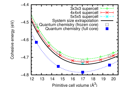
Figure 1: Cohesive energy as a function of primitive cell volume for the extrapolated pp-DMC calcualtions and the quantum chemistry calculations with and without core-valence correlation effects. DMC calculations on finite supercells are included to show convergence. The lines indicate a Birch–Murnaghan fit to the data.

The values of $E_{\rm coh}$, $a_{0}$ and $B_{0}$ obtained from the fit are given in Table 1. Several important points emerge from these results. First, the system-size effects consist almost entirely of a vertical shift, i.e. a constant energy offset, of the $E_{\rm coh}(V)$ curves, so that they cause only small errors in $a_{0}$ and $B_{0}$. For example going from the $3\times 3\times 3$ supercell to the extrapolated system changes $a_{0}$ by only $\sim 0.1$ %. Second, comparing the raw values of $E_{\rm coh}$ from DMC on the $3\times 3\times 3$ and $4\times 4\times 4$ supercells to the fully-corrected and extrapolated value suffers from substantial errors of 133 and 52 meV, the KZK correction reduced these to 50 and 22 meV respectively. Third, the DMC value of $E_{\rm coh}$, even after correction, still disagrees with the quantum chemistry value of $E_{\rm coh}$ without core correlation energy by $\sim 36$ meV. This last point indicates that the effect of the pseudopotential approximation must be significant. In order to make further progress, all-electron DMC is needed, and we report on this next.

Table 1: Calculated bulk properties with both pseudopotential and all–electron DMC and hierarchical quantum chemistry with and without core effects. The cohesive energy is calculated at 4.084Å  in all cases.

	$a_{0}$ / Å		$B_{0}$ / GPa		$E_{\mathrm{coh}}$ / eV
DMC 3$\times$3$\times$3	4.	0965(2)	30	.5(1)	$-$4.	6967(1)
DMC 4$\times$4$\times$4	4.	096(2)	31	.1(8)	$-$4.	7249(1)
DMC Extrap.	4.	093(2)	31	(1)	$-$4.	7466(3)
DMC all–electron	4.	061(1)	31	.8(4)	$-$4.	758(1)
Quantum Chemistry (no core)nolan_calculation_2009	4.	099	31	.9	$-$4.	7087
Quantum Chemistry (with core)nolan_calculation_2009	4.	062	33	.1	$-$4.	7710
Experimentnolan_calculation_2009	4.	061(1)	33	-38	$-$4.	778,$-$4.759

III.2 All-electron calculations

In order to perform accurate all-electron DMC on the LiH crystal, we have to address several technical challenges. First, as noted in Sec. II.1, the trial wavefunction must accurately satisfy the Kato cusp condition at the nucleus, in order to ensure stability of the walker population. Second, because of the rapid variation of the orbitals near the nucleus, extremely fine blip-grids are needed. Third, we expect to need much shorter time-steps than for pseudopotential calculations.

The technique used to ensure that the cusp condition is satisfied is outlined in Appendix A. One symptom of the rapid variation of the orbitals near the nucleus is the slow convergence of the DFT total energy with respect to plane-wave cut-off in the quantum espresso calculations used to generate the orbitals. Given the high memory requirements caused by the high cut-offs in the DMC calculations, we took the orbitals to be sufficiently converged when they produced stable walker populations. For our final all-electron DMC calculations, we used orbitals generated using the LDA functional, with a plane-wave cut-off of $6.8\times 10^{4}$ eV. The associated blip-grid had a spacing of half the natural grid dictated by the plane-wave cut-off.

We made detailed tests on the time-step needed to ensure the accuracy of the all-electron calculations. In Fig. 2, we show the results of tests on the $3\times 3\times 3$ supercell, showing how the total energy converges with respect to time step. The figure also shows a linear fit to the results, which is clearly adequate, as expected from earlier work.rothstein_time_1987 A time step of $0.004$ au gives an error of only 10 meV/formula unit, which more than suffices to give accurate results for the equilibrium $a_{0}$ and $B_{0}$.

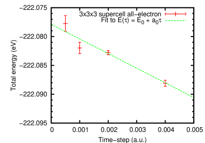
Figure 2: Total energy vs. time–step. This shows the convergence of the ae-DMC calculations with respect to time–step and is for a 3$\times$3$\times$3 supercell. A linear extrapolation to zero timestep is included.

In order to obtain the best possible results for the cohesive energy as a function of volume $E_{\rm coh}(V)$, we used the fact made clear in Sec. III.1 that results with the $3\times 3\times 3$ supercell differ only by an almost constant energy offset from results converged with respect to supercell size, this offset being in the region of 30 meV. Our procedure in the all-electron DMC calculations was therefore to calculate $E_{\rm coh}(V)$ first with the $3\times 3\times 3$ supercell and a time step of $0.004$ au. We then added a constant correction energy to these results, obtained from DMC calculations with time steps of $0.001$, $0.002$ and $0.004$ au, all performed on both the $3\times 3\times 3$ and $4\times 4\times 4$ supercells. At each time step, the usual two-point extrapolation (Eq. (4)) to infinite supercell size was made, and a final linear time-step extrapolation was then made.

The cohesive energy curve from all-electron DMC is compared in Fig. 3 with our pseudopotential DMC curve and the results from quantum chemistry. The resulting equilibrium values of $E_{\rm coh}$, $a_{0}$ and $B_{0}$ are compared in Table 1. We see that the all-electron DMC value of $a_{0}$ agrees with the experimental and quantum chemistry values to within $\sim 10^{-3}$ Å ($0.03$ %). Values of $B_{0}$ are much more difficult to obtain accurately, but the all-electron DMC value agrees with quantum chemistry to within $\sim 4$ %, and both are reasonably consistent with experimental values, which span a range of $\sim 15$ %. The all-electron DMC and quantum chemistry values of the equilibrium $E_{\rm coh}$ differ by $13$ meV/formula unit. The quantum chemistry value is believed to be somewhat more accurate than this, so that some of this $13$ meV may be due to fixed-node error.

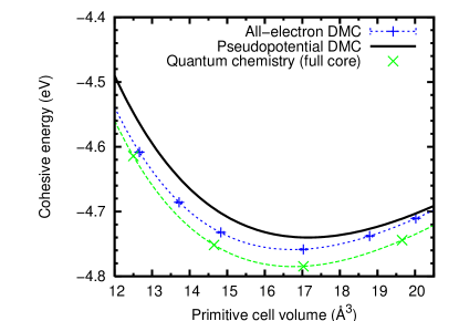
Figure 3: Cohesive energy vs. primitive cell volume. Here the DMC energy differences have been calculated using a 3$\times$3$\times$3 supercell and timestep of 0.004 a.u. and the point at 17.03ų calculated using the extrapolation procedure in the text.

IV Surface formation energy of LiH with QMC

The methods of Secs. II.1 and II.2 have been used to calculate the formation energy of the LiH (001) surface, first with pseudopotentials, then with all-electron DMC. All the calculations were done with the lattice parameter $a_{0}=4.084$ Å.

IV.1 Pseudopotential calculations

Exactly the same pseudopotential methods were used for the calculations on slabs as were used in the bulk calculations of Sec. III.1, and the trial orbitals were generated using DFT with the LDA functional, as before. These orbitals were then re-expanded in B-splines using a spacing corresponding to $\pi/2k_{\rm max}$ where $k_{\rm max}$ is the modulus of the largest plane-wave vector. For each surface supercell and each number $N$ of ionic layers, the Jastrow factor of 1-, 2- and 3-body terms was re-optimized using variance minimization.

To extract the values of $\sigma$ and $E_{\rm layer}$ for each chosen surface unit cell, we performed calculations of the total slab energy $E_{\rm slab}(N)$ for numbers of ionic layers from 3 to 6 using a $4\times 4$ surface unit cell (18 ions per layer in the repeating supercell). Single-particle size errors were corrected for using Eq. (2) with $a$ set equal to 1. Table 2 shows the convergence of $\sigma$ with respect to the slabs used when fitting to Eq. (6). We have also performed calculations for slabs 3 and 4 using a $3\times 3$ surface unit cells (18 ions per layer in the repeating supercell). Comparing directly the $\sigma_{3,4}$ from the two different surface unit cells differed by only 0.006(5) J m^-2 indicating the finite–size error. The resulting best value for $\sigma$ from the pseudopotential calculations is 0.373 J m^-2.

Table 2: pp-DMC surface formation energy calculated using slabs of different thicknesses. Calculations performed on $4\times 4$ surface unit cells.

Slabs used	$\sigma~{}/$ J m-2
3,4,5,6	0	.369(2)
4,5,6	0	.373(3)
5,6	0	.379(6)

IV.2 All-electron calculations

The all-electron DMC techniques used for the slab calculations were essentially the same as those used for the bulk (Sec. III.2). However, the memory requirements for the B-spline coefficients were so much greater than for the bulk that we had to reduce the plane-wave cut-off used to generate the orbitals from $6.8\times 10^{4}$ to $3.4\times 10^{4}$ eV. This primarily made the DMC runs more susceptible to population control issues and resulted in a higher statistical error on the final values compared to the pseudopotential work. For the same reason, were able to perform all-electron calculations only for the $3\times 3$ surface unit cell, and the largest number of ionic layers that we could handle was $N=5$. We know from the pseudopotential calculations that the finite size errors are under control using $3\times 3$ surface unit cells assuming the LDA correction is used. The introduction of the tightly bound core electrons is not expected to increase the finite-size errors.

A further technical issue in the all-electron slab calculations was concerned with the optimization of the Jastrow factor. In order to obtain wavefunctions that produced stable DMC runs we found it necessary to optimize the Jastrow factor using the energy minimisation scheme within VMC. This tended to increase the variance of the local energy of the trial wavefunction slightly with respect to variance minimisation. However it did reduce the number of population explosions during the DMC runs.

The timestep adopted ($0.004$ a.u.) was the same as used in the all-electron bulk work, since the tests done there indicated that this is sufficient. Our final all-electron DMC result for the surface formation energy is $\sigma=0.44(1)~{}\rm J\,m^{-2}$. We note that the explicit inclusion of Li core states increases $\sigma$ by $\sim 0.07$ J m^-2, which is a significant effect at the level of accuracy sought in this work.

V Hierarchical quantum chemistry for surface energy

The formation energy of the of LiH (001) surface was also computed using quantum chemistry techniques. The Hartree-Fock component $\sigma^{\mathrm{HF}}$ was determined from slab calculations, see Eq. (6), using the CRYSTAL and VASP codes. The effect of electron correlation was accounted for using the hierarchical method as described in Section II.3.

Both CRYSTAL and VASP employ periodic boundary conditions, so that the calculations are performed on an infinite array of slabs, with a vacuum gap separating successive slabs. The vacuum gap was chosen to be 26 Å, large enough to ensure that there is no interaction between neighbouring slabs. Careful attention was also paid to convergence with respect to $k$-point sampling and basis-set completeness. A previous high accuracy Hartree-Fock study of bulk LiH was performed using CRYSTAL by Paier et alpaier_accurate_2009 . The basis set described in that work was used for the present calculations. In order to ensure basis set completeness, layers of “ghost” atoms were added above and below each surface. The “ghost” atoms were basis functions centred on the sites of atoms in the next layer but without the nuclei or electrons. The convergence of $\sigma^{\mathrm{HF}}$ with respect to these “ghost” atoms was tested using slabs of four and five layers, see Table 3. The introduction of the “ghost” atoms has a significant effect on $\sigma^{\mathrm{HF}}$ and two layers are necessary to achieve basis set completeness; this number of layers was used in all our calculations.

Table 3: Convergence of $\sigma_{\mathrm{HF}}$ using CRYSTAL with respect to the number of layers of “ghost” atoms above and below the surface. Based on two-point extrapolations from slabs of 4-5 layers. All energies are quoted in J m^-2.

Ghost layers	$\sigma_{\mathrm{HF}}$
0	0.43835
1	0.19886
2	0.19849
3	0.19854

Calculations on slabs of two to eight layers were performed using both periodic codes, and the method outlined in Sec. IV.1 was used to extract values of $\sigma^{\rm HF}$. The resulting values are shown in Table 4. We note that the VASP value is slightly lower than the CRYSTAL value. Since CRYSTAL provides a direct all-electron calculation, and we have established that the CRYSTAL result is converged with respect to basis set, we suggest that the VASP value may be a slight underestimate. This may be due to the PAW potentials used: the standard PBE potentials were used, and while harder potentials are available for H, it was not possible to reach convergence with these potentials. Previous studies of bulk LiH with VASP have reported small discrepancies in the Hartree-Fock result marsman_second-order_2009 . The CRYSTAL results converge with respect to slab thickness to give a value of 0.198(1) J m^-2.

Table 4: Hartree-Fock approximation to surface formation energy for LiH, $a=4.084$ Å, using CRYSTAL and VASP. All energies are quoted in J m^-2.

Slabs used	CRYSTAL	VASP
2-8	0.20005	0.19363
3-8	0.19883	0.19114
4-8	0.19825	0.19001
5-8	0.19819	0.18944
6-8	0.19836	0.18926
7-8	0.19703	0.18864

The correlation component of the surface formation energy was calculated using the hierarchical method. The convergence of the hierarchical coefficients is shown in Fig. 4 and using the methods described in Ref. nolan_calculation_2009, the values can be converged to within a few tenths of mE_h. In brief, a reference calculation was performed using $N=64$ and frozen-core MP2 theory in the cc-pVTZ basis set. Corrections for core correlation ($\delta$core), basis-set incompleteness ($\delta$basis) and higher-level correlation treatments ($\delta$CCSD(T), $\delta$CCSDT, $\delta$CCSDT(Q)) and the diagonal Born-Oppenheimer correction were also computed using smaller basis sets and smaller values of $N$. The use of smaller values of $N$ for small corrections was validated in earlier work nolan_calculation_2009 . Complete details of the hierarchical results are given in Table 5. An error of 0.2 mE_h in the hierarchical coefficients corresponds to an error of 0.005 J m^-2 in the surface formation energy. To facilitate comparison with both DMC results, $\sigma^{\mathrm{corr}}$ has been calculated with and without correlating the core electrons.

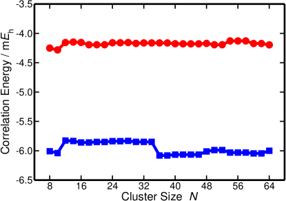
Figure 4: The convergence of $E^{011}$ (red circles) and $E^{111}$ (blue squares) with respect to maximum cluster size $N$ using MP2/cc-pVTZ for LiH $a=4.084$ Å

Table 5: Correlation contributions to the surface formation energy of LiH at $a=4.084$ Å and total calculated surface formation energies with and without core correlation. In each row, the $N$ value specifies the maximum number of ions in the hierarchical calculation. Correlation-consistent basis sets have been used throughout, and cc-p(C)V$X$Z is abbreviated (C)V$X$Z. The CCSDT and CCSDT(Q) calculations were performed using MRCC kallay ; mrcc as a module in Molpro and the diagonal Born-Oppenheimer correction (DBOC) calculations were performed using PSI3 psi3 . All other calculations were performed using Molpro molpro .

reference	$E^{011}$/m$E_{\rm h}$	$E^{111}$/m$E_{\rm h}$	$\sigma^{\mathrm{corr}}$/J m-2	details
	$-4.196$	$-6.000$	+0.1886	MP2/VTZ $N=64$
$\delta$core	$-0.840$	$-1.147$	+0.0321	MP2/CVTZ $-$ MP2/VTZ $N=16$
$\delta$basis	+0.268	+0.268	$+0.0000$	MP2/V[T,Q]Z $N=36$
	+0.162	+0.158	$+0.0004$	MP2/V[Q,5]Z $N=16$
$\delta$CCSD(T)	+0.625	+0.538	+0.0091	CCSD(T)/VTZ $-$ MP2/VTZ $N=16$
$\delta$CCSDT	$-0.149$	$-0.209$	+0.0063	CCSDT/VDZ $-$ CCSD(T)/VDZ $N=8$
$\delta$CCSDT(Q)	$-0.015$	$-0.023$	+0.0008	CCSDT(Q)/VDZ $-$ CCSDT/VDZ $N=8$
DBOC	+0.041	+0.055	$-0.0015$	HF/VTZ $N=8$
$\sigma^{\mathrm{corr}}_{\mathrm{frozen~{}core}}$			0.2037	Sum terms above except $\delta{}$core
$\sigma^{\mathrm{corr}}_{\mathrm{total}}$			0.2358	Sum all terms above
$\sigma^{\mathrm{HF}}$			$0.198\phantom{0}$
$\sigma^{\mathrm{static}}_{\mathrm{frozen~{}core}}$			$0.402\phantom{0}$
$\sigma^{\mathrm{static}}_{\mathrm{total}}$			$0.434\phantom{0}$

VI Discussion

We summarize in Table 6 our QMC and hierarchical quantum chemistry results for the formation energy $\sigma$ of the LiH (001) surface, and we compare with the predictions of DFT using the LDA, PBE and rPBE functionals, these DFT results being taken from our earlier work binnie_benchmarking_2009 . The very close agreement between the DMC and QC results for $\sigma$ confirms that both approaches give high accuracy, and shows that the results can be used as benchmarks for assessing DFT approximations. The DFT values of $\sigma$ span a remarkably wide range, with LDA overestimating it by $7$ %, and PBE and rPBE underestimating it by $23$ % and nearly $40$ % respectively. It is interesting to note that the Hartree-Fock value $\sigma^{\rm HF}$ of $0.20$ J m^-2 (Table 4) accounts for less than half the full value of $\sigma$, so that the importance of an accurate treatment of correlation is clear. It is also noteworthy that valence-core correlation gives a surprisingly significant contribution of $\sim 10$ % to $\sigma$. We noted in the Introduction the scattered evidence that LDA tends to give better values of $\sigma$ than GGA approximations, and the present work shows that this is the case for LiH.

Table 6: Calculated surface formation energy with both pseudopotential and all–electron DMC and hierarchical quantum chemistry with and without core effects. The calculations are performed at 4.084Å  in both cases. DFT data from previous work is included. The DFT values are for the lattice parameters optimized with the given functionals.binnie_benchmarking_2009

method	$\sigma$ / J m-2
DMC pseudopotential	0.	373(3)
DMC all–electron	0.	44(1)
Quantum Chemistry (froz. core)	0.	402
Quantum Chemistry (with core)	0.	434
DFT LDA	0.	466
DFT PBE	0.	337
DFT rPBE	0.	272

An important part of the evidence that our DMC and hierarchical QC calculations give results of benchmark quality for $\sigma$ is the very high accuracy of the two completely independent approaches for the energetics of the LiH crystal; for hierarchical quantum chemistry, this was already shown in detail in Ref. nolan_calculation_2009, , and a substantial part of the present paper has been devoted to showing the same thing for QMC. In both approaches, the calculated cohesive energy is correct to $\sim 15$ meV/formula unit, and the equilibrium lattice parameter to within better than $0.1$ %. It is clear from both sets of calculations that an adequate treatment of core-valence correlation must be included. The reliability of the calculated values for $\sigma$ is confirmed by the very close agreement (within $\sim 0.01$ J m^-2) between the values given by the two approaches. Here too, core-valence correlation is important, giving a contribution of $\sim 0.03$ J m^-2 to $\sigma$.

In both theoretical approaches, a key technical issue is system size effects. In QMC, the calculations are done directly in periodic boundary conditions, but large repeated systems are needed because we rely on $\Gamma$-point sampling. For the bulk crystal, we have shown that significant corrections need to be made for size errors, but that these are successful in reducing the errors in the cohesive energy to $\sim 15$ meV/formula unit. For the DMC slab calculations of $\sigma$, we have presented evidence that the calculated $\sigma$ is very well converged (to within 0.006 J m^-2) with respect to both slab thickness and size of the surface repeating unit. In the hierarchical approach, the Hartree-Fock part of $\sigma$ is calculated in periodic boundary conditions, and we have shown that size errors in the slab calculations can be made negligible. Size errors in the correlation residual contributions are well controlled in the hierarchical scheme, and, as can be seen from Fig. 4, are of the order of 0.1 ${\rm m}E_{\rm h}$ per ion.

It would now be timely to extend the present calculations to other materials. In fact, we have reported QMC calculations of $\sigma$ for MgO (001) several years ago alf_energetics_2006 , though it might be worth repeating the calculations with the improved pseudopotentials now available. Our hierarchical quantum chemistry scheme can be applied without change to MgO and other materials having the rock-salt structure, and we hope to report both QMC and hierarchical calculations on LiF in the near future. However, it is important to emphasise that the hierarchical scheme also works well for materials having other crystal structures, so that there is now rather wide scope for using it, with or without QMC, for calculations of $\sigma$. We remark that for some materials it will be essential to include the effects of surface relaxation. This is not a significant issue for most rock-salt materials, and we have shownbinnie_benchmarking_2009 that for LiH relaxation reduces $\sigma$ by only $\sim 0.01$ J m^-2. But in other cases (corundum is a famous example), relaxation makes a large difference to $\sigma$, and would probably need to be estimated from DFT calculations.

To conclude, we have shown that: (a) quantum Monte Carlo calculations give extremely accurate results for the energetics of the LiH crystal, particular when Li core electrons are explicitly included, and there is excellent agreement with results from the hierarchical quantum chemistry scheme; (b) these two independent techniques give almost identical benchmark results for the formation energy of the LiH (001) surface; (c) the benchmark value of $\sigma$ lies between DFT predictions from the LDA and GGA approximations, the LDA value being somewhat better than GGA.

Appendix A Generalised cusp correction

A scheme for modifying real orbitals expanded in a Gaussian basis set so that they satisfy the Kato cusp conditionskato_eigenfunctions_1957 ; pack_cusp_1966 is described in Ref. ma_scheme_2005, . In the present work we make use of an extension of this scheme which allows the Kato cusp conditions to be imposed on complex orbitals expanded in any smooth basis set.

For simplicity, we restrict our attention to the case of an all-electron nucleus of charge $Z$ at the origin in the following discussion. In the scheme of Ref. ma_scheme_2005, , the s-type Gaussian basis functions are replaced by radial functions in the vicinity of the nucleus. These functions impose the cusp conditions and make the single-particle local energy resemble an “ideal” curve that was found empirically to be satisfied by a wide range of Hartree-Fock atomic orbitals. In the scheme used in this work, instead of replacing part of the orbital, we add a spherically symmetric function of constant phase to the orbital. The function added to uncorrected orbital $\psi({\bf r})$ is

$$\Delta\psi(r)=\exp(i\theta_{0})\left[\tilde{\phi}(r)-\phi(r)\right]\Theta(r_{c}-r),$$ (14)

where $\Theta$ is the Heaviside function, $r_{c}$ is a cutoff length, $\theta_{0}=\arg[\psi({\bf 0})]$,

$$\phi(r)={\rm Re}\left[\frac{\exp(-i\theta_{0})}{4\pi}\int_{\rm sphere}\psi({\bf r})\,d\Omega\right],$$ (15)

and

$$\tilde{\phi}(r)=C+\exp(\alpha_{0}+\alpha_{1}r+\alpha_{2}r^{2}+\alpha_{3}r^{3}+\alpha_{4}r^{4}),$$ (16)

where $C$ is a real constant and the $\{\alpha\}$ are real constants to be determined. In practice $\phi(r)$ is evaluated by cubic spline interpolation; the spherical averaging of the uncorrected orbital is performed on a radial grid at the outset of the calculation. $C$ is chosen so that $\phi(r)-C$ is positive everywhere within the Bohr radius of the nucleus.

The uncorrected orbital may be written as

$$\psi({\bf r})=\exp(i\theta_{0})\phi(r)+\eta({\bf r}),$$ (17)

where $\eta({\bf r})$ consists of the $l>0$ spherical harmonic components of $\psi({\bf r})$, together with the phase-dependence of the $l=0$ component. Note that $\exp(i\theta_{0})\phi(0)=\psi({\bf 0})$, and hence $\eta({\bf 0})=0$. We may now apply the scheme of Ref. ma_scheme_2005, to determine $\{\alpha\}$ and $r_{c}$, with $\exp(i\theta_{0})\phi$ and $\exp(i\theta_{0})\tilde{\phi}$ playing the roles of the uncorrected and corrected s-type Gaussian functions centered on the nucleus at the origin. The constant phase $\exp(i\theta_{0})$ cancels out of the equations that determine the $\{\alpha\}$ [Eqs. (9)–(13) in Ref. ma_scheme_2005, ], so the determination of the $\{\alpha\}$ and $r_{c}$ is exactly as described in Ref. ma_scheme_2005, , except that we do not need to modify $Z$ when more than one nucleus is present, because $\eta({\bf 0})=0$.

Suppose the orbital is of Bloch form $\psi({\bf r})=u_{\bf k}({\bf r})\exp(i{\bf k}\cdot{\bf r})$, where $u_{\bf k}$ has the periodicity of the primitive cell. Let $\{{\bf R}_{p}\}$ be the set of primitive-cell lattice points. The orbital may be corrected at each all-electron nucleus in the primitive cell at ${\bf R}_{p}={\bf 0}$ using the scheme described above. The phase of the orbital (and hence cusp-correction function) at the corresponding nucleus in the primitive cell at ${\bf R}_{p}\neq{\bf 0}$ is $\exp(i{\bf k}\cdot{\bf R}_{p})$ times that for the primitive cell at ${\bf R}_{p}={\bf 0}$; the cusp-correction function is otherwise identical. The corrected orbital is of Bloch form.

References

- (1) J. Goniakowski, J. M. Holender, L. N. Kantorovich, M. J. Gillan, and J. A. White, Phys. Rev. B 53, 957 (1996).
- (2) A. E. Mattsson and D. R. Jennison, Surf. Sci. 520, L611 (2002).
- (3) D. Yu and M. Scheffler, Phys. Rev. B 70, 155417 (2004).
- (4) S. J. Binnie, E. Sola, D. Alfè, and M. J. Gillan, Mol. Sim. 35, 609 (2009).
- (5) D. Alfè and M. J. Gillan, J. Phys.: Condens. Matt. 18, L435 (2006).
- (6) L. M. Almeida, J. P. Perdew, and C. Fiolhais, Phys. Rev. B 66, 075115 (2002).
- (7) W. M. C. Foulkes, L. Mitáš, R. J. Needs, and G. Rajagopal, Rev. Mod. Phys. 73, 33 (2001).
- (8) R. J. Needs, M. D. Towler, N. D. Drummond, and P. López Ríos, J. Phys.: Condens. Matt. 22, 023201 (2010).
- (9) H. Stoll, Phys. Rev. B 46, 6700 (1992).
- (10) B. Paulus, Phys. Rep. 428, 1 (2006).
- (11) M. Marsman, A. Grüeneis, J. Paier, and G. Kresse, J. Chem. Phys. 130, 184103 (2009).
- (12) C. Pisani et al., J. Comp. Chem. 29, 2113 (2008).
- (13) S. J. Nolan, M. J. Gillan, D. Alfè , N. L. Allan, and F. R. Manby, Phys. Rev. B 80, 165109 (2009).
- (14) F. R. Manby, D. Alfè, and M. J. Gillan, Physical Chemistry Chemical Physics 8, 5178 (2006).
- (15) D. M. Ceperley and B. J. Alder, Phys. Rev. Lett. 45, 566 (1980).
- (16) J. B. Anderson, J. Chem. Phys. 63, 1499 (1975).
- (17) J. R. Trail and R. J. Needs, J. Chem. Phys. 122, 174109 (2005).
- (18) J. R. Trail and R. J. Needs, J. Chem. Phys. 122, 014112 (2005).
- (19) L. Mitáš, E. L. Shirley, and D. M. Ceperley, J. Chem. Phys. 95, 3467 (1991).
- (20) P. R. C. Kent, R. Q. Hood, M. D. Towler, R. J. Needs, and G. Rajagopal, Phys. Rev. B 57, 15293 (1998).
- (21) J. Ma, D. Alfè, A. Michaelides, and E. Wang, J. Chem. Phys. 130, 154303 (2009).
- (22) P. Giannozzi et al., J. Phys.: Condens. Matt. 21, 395502 (19pp) (2009).
- (23) D. Alfè and M. J. Gillan, Phys. Rev. B 70, 161101 (2004).
- (24) L. M. Fraser et al., Phys. Rev. B 53, 1814 (1996).
- (25) A. J. Williamson et al., Phys. Rev. B 55, R4851 (1997).
- (26) P. R. C. Kent et al., Phys. Rev. B 59, 1917 (1999).
- (27) H. Kwee, S. Zhang, and H. Krakauer, Phys. Rev. Lett. 100, 126404 (2008).
- (28) D. M. Ceperley and B. J. Alder, Phys. Rev. B 36, 2092 (1987).
- (29) G. Rajagopal, R. J. Needs, A. James, S. D. Kenny, and W. M. C. Foulkes, Phys. Rev. B 51, 10591 (1995).
- (30) F. H. Zong, C. Lin, and D. M. Ceperley, Physical Review E 66, 036703 (2002).
- (31) J. P. Perdew, K. Burke, and M. Ernzerhof, Phys. Rev. Lett. 77, 3865 (1996).
- (32) S. M. Rothstein, N. Patil, and J. Vrbik, J. Comp. Chem. 8, 412 (1987).
- (33) J. Paier et al., Phys. Rev. B 80, 174114 (2009).
- (34) M. Marsman, A. Grüneis, J. Paier, and G. Kresse, J. Chem. Phys. 130, 184103 (2009).
- (35) M. Kállay and P. R. Surján, J. Chem. Phys. 115, 2945 (2001).
- (36) M. Kállay, MRCC, a string-based quantum chemical program suite, see http://www.mrcc.hu.
- (37) T. D. Crawford et al., J. Comp. Chem. 28, 1610 (2007).
- (38) H.-J. Werner, P. J. Knowles, R. Lindh, F. R. Manby, M. Schütz and others., Molpro, version 2008.1, a package of ab initio programs, 2008, see http://www.molpro.net.
- (39) T. Kato, Comm. Pure App. Math. 10, 151 (1957).
- (40) R. T. Pack, J. Chem. Phys. 45, 556 (1966).
- (41) A. Ma, M. D. Towler, N. D. Drummond, and R. J. Needs, J. Chem. Phys. 122, 224322 (2005).