Dark matter scaling relations in intermediate $z$ haloes

Abstract

We investigate scaling relations between the dark matter (DM) halo model parameters for a sample of intermediate redshift early - type galaxies (ETGs) resorting to a combined analysis of Einstein radii and aperture velocity dispersions. Modeling the dark halo with a Navarro - Frenk - White profile and assuming a Salpeter initial mass function (IMF) to estimate stellar masses, we find that the column density ${\cal{S}}$ and the Newtonian acceleration within the halo characteristic radius $r_{s}$ and effective radius $R_{eff}$ are not universal quantities, but correlate with the luminosity $L_{V}$, the stellar mass $M_{\star}$ and the halo mass $M_{200}$, contrary to recent claims in the literature. We finally discuss a tight correlation among the DM mass $M_{DM}(R_{eff})$ within the effective radius $R_{eff}$, the stellar mass $M_{\star}(R_{eff})$ and $R_{eff}$ itself. The slopes of the scaling relations discussed here strongly depend, however, on the DM halo model and the IMF adopted so that these ingredients have to be better constrained in order to draw definitive conclusions on the DM scaling relations for ETGs.

1 Introduction

The current cosmological paradigm, the concordance $\Lambda$CDM model, relies on two main components, namely dark energy (e.g. Carroll et al. 1992) and dark matter. Although in excellent agreement with all the cosmological probes (Komatsu et al. 2009; Percival et al. 2009; Lampteil et al. 2009), the $\Lambda$CDM model is nevertheless afflicted by serious problems on galactic scales. In this framework, the formation of virialized DM haloes from the initial tiny density perturbations is followed at later stages through numerical N - body simulations (Bertschinger 1998). It became apparent that the spherically averaged density profile, $\rho_{DM}(r)$, of DM haloes is independent of the halo mass (Navarro et al. 1997) and well described by a double power - law relation with $\rho_{DM}\propto r^{-3}$ in the outer regions and $\rho_{DM}\propto r^{-\alpha}$ with $\alpha>0$ centrally. On the contrary, observations of spiral galaxies seem to definitely point towards cored models, i.e. $\alpha=0$ at the centre (de Blok 2009). Understanding whether such a discrepancy is due to some physical process not correctly modeled in simulations or to a failure of the CDM paradigm is still a hotly debated issue. As a valuable tool to address this problem, one can look for scaling relations among DM halo parameters and stellar quantities in order to better constrain the formation scenario and the DM properties. Recently, much work has been dedicated to this issue. Using a sample of local ETGs, Tortora et al. (2009, T09 hereafter) have found that DM is the main driver of the Fundamental plane (FP) tilt (see also Cappellari et al. 2006, Bolton et al. 2007, Hyde & Bernardi 2009, Graves & Faber 2010, Auger et al. 2010b) and that the average spherical DM density is a decreasing function of stellar mass (see also Thomas et al. 2009). Based on data from rotation curves of $\sim 1000$ spiral galaxies, the mass models of individual dwarf and spiral galaxies and the weak lensing signal of elliptical and spirals, Donato et al. (2009, D09) and Gentile et al. (2009, G09) have found strong evidence for the constancy of the central DM column density over 12 orders of magnitude in luminosity. Napolitano, Romanowsky & Tortora (2010, NRT10) have shown that, on average, the projected density of local ETGs within effective radius is systematically higher than the same quantity for spiral and dwarf galaxies, pointing to a systematic increase with halo mass as suggested by Boyarsky et al. (2009a, B09), who have extended the samples analyzed above to both group and cluster scale systems.

In order to try to discriminate between these contrasting results, we present here an analysis of the DM scaling relations for a sample of ETGs at intermediate redshift ($\langle z\rangle\simeq 0.2$) using lensing and velocity dispersion data to constrain their parameters. The mass models, the data and the fitting procedure are described in §2. In §3 we describe the main results, while §4 is devoted to a brief review of the results and conclusions.

2 Estimating mass quantities

As a preliminary mandatory step, we need to determine the quantities involved in the above scaling relations. To this end, one has first to choose a model for the stellar and DM components and then fit the observational data in order to infer the quantities of interest from the constrained model.

2.1 Stellar and DM profiles

Motivated by the well known result that the surface brightness profiles of ETGs are well fitted by the S$\rm\acute{e}$rsic (1968) law, we describe the stellar component with the Prugniel & Simien (1997, PS hereafter) profile (see also Marquez et al. 2001 for further details). The choice of the DM halo model is quite controversial. Rotation curves of $z=0$ spiral galaxies are better fitted by cored models (de Blok 2009), but we are here considering ETGs at intermediate $z$ so that it is not straightforward to extend these results to our case. In order to explore the impact of the DM halo profile, we therefore adopt both a Burkert (1995) model with

$$\rho_{B}(r)=\frac{\rho_{B}r_{B}^{3}}{(r+r_{B})(r^{2}+r_{B}^{2})}\ ,$$ (1)

and an NFW (Navarro et al. 1997) profile with

$$\rho_{NFW}(r)=\frac{\rho_{s}r_{s}^{3}}{r(r+r_{s})^{2}}\ .$$ (2)

Both the 3 - dimensional and projected masses $M(r)$ and $M_{proj}(R)$ can be analytically evaluated, with $M_{proj}(R)$ given in Park & Ferguson (2003) and Bartelmann (1996) for the Burkert and NFW models, respectively.

In order to constrain the model parameters, we rely on the estimate of the projected mass $M_{E}=M_{proj}(R_{E})$ inferred by the measurement of the Einstein radius $R_{E}$ in a lens system. While lensing probes the mass projected along the line of sight, the aperture velocity dispersion $\sigma_{ap}$ (Mamon & Lokas, 2005) provides complementary information on the internal dynamics thus strengthening the constraints.

2.2 Data and fitting procedure

We make use of the sample of 85 lenses collected by the Sloan Lens ACS (SLACS) survey (Auger et al. 2009) and first select only ETGs with available values of both the velocity dispersion $\sigma_{ap}$ (measured within an aperture of $R_{\rm ap}=1.5^{\prime\prime}$) and the Einstein radius $R_{E}$, thus ending up with a dataset containing 59 objects. For each lens, we follow Auger et al. (2009) setting the S$\rm\acute{e}$rsic index $n=4$ and the effective radius $R_{eff}$ and total luminosity $L_{V}$ to the values inferred from the $V$ - band photometry. The SLACS collaboration has also provided an estimate of the total stellar mass (their Table 4) from which we use both Chabrier (2001) and Salpeter (1955) IMFs to investigate the effect of the IMF on the scaling relations.

Before fitting the model to the data, it is worth noting that, for both the Burkert and NFW models, the halo parameters are different from one lens to another. Since we have only two observed quantities, namely $(M_{E},\sigma_{ap})$ for each lens, determining $(\rho_{X},r_{X})$ (with $X=B$ or $s$ for the Burkert and NFW models, respectively) on a case - by - case basis would give us very weak constraints. We therefore bin the galaxies in 10 equally populated luminosity bins (the last one actually containing 5 objects) and resort to a different parametrization using quantities that it can be reasonably assumed to be the same for all the lenses in the same bin. As one of the fitting parameters, we choose the virial $M/L$ ratio, $\Upsilon_{vir}=M_{vir}/L_{V}$ with $M_{vir}$ the DM halo mass at the virial radius $R_{vir}$. Should $\Upsilon_{vir}$ depend on $L_{V}$, our luminosity bins are quite narrow so that any change in $\Upsilon_{vir}$ should be so small that can be safely neglected. We then use $\log{\eta_{X}}$ with $\eta_{X}=r_{X}/R_{eff}$ as the second parameter.

Note that, although $(\Upsilon_{vir},\log{\eta_{X}})$ are the same for all the galaxies in a bin, $(M_{vir},r_{X})$ still change from one lens to another thus allowing us to estimate all the quantities of interest on a lens - by - lens basis. In order to constrain $(\Upsilon_{vir},\log{\eta_{X}})$, we maximize a suitable likelihood function, composed of two terms, the first (second) one referring to the lensing (dynamics) constraints (see Cardone et al. 2009 for further details). In order to efficiently explore the parameter space, we use a Markov Chain Monte Carlo (MCMC) algorithm running chains with 100000 points reduced to more than 3000 after burn in cut and thinning. For a given galaxy, we compute the quantities of interest for each point in the chains and then use Bayesian statistics to infer median values and $68\%$ confidence intervals. We follow D’ Agostini (2004) to correct for the asymmetric errors in our estimates.

3 Results

Before investigating scaling relations, it is worth checking whether our PS + DM model works in fitting the lens data.

Table 1: Constraints on halo parameters for the Burkert models with Chabrier and Salpeter IMF. The median luminosity from the galaxies in each bin is reported in column 1, while the adjacent columns give the maximum likelihood parameter $(\Upsilon_{vir},\log{\eta_{s}})_{ML}$, the value of $-2\ln{{\cal{L}}}$ at the maximum, median value and $68$ per cent confidence interval for the DM parameters $(\Upsilon_{vir},\log{\eta_{s}})$ for each model.

Bin	Chabrier IMF				Salpeter IMF
$\log{L_{V}}$	$(\Upsilon_{vir},\log{\eta_{s}})_{ML}$	$-2\ln{{\cal{L}}_{max}}$	$(\Upsilon_{vir})_{-1\sigma}^{+1\sigma}$	$(\log{\eta_{s}})_{-1\sigma}^{+1\sigma}$	$(\Upsilon_{vir},\log{\eta_{s}})_{ML}$	$-2\ln{{\cal{L}}_{max}}$	$(\Upsilon_{vir})_{-1\sigma}^{+1\sigma}$	$(\log{\eta_{s}})_{-1\sigma}^{+1\sigma}$
10.72	$(15,-0.61)$	353.179	$26_{-12}^{+22}$	$-0.38_{-0.24}^{+0.21}$	$(15,-0.80)$	351.645	$19_{-11}^{+32}$	$-0.24_{-0.32}^{+0.19}$
10.82	$(53,-0.18)$	362.797	$46_{-32}^{+60}$	$-0.22_{-0.22}^{+0.22}$	$(35,-0.15)$	364.679	$41_{-23}^{+30}$	$-0.09_{-0.25}^{+0.15}$
10.85	$(9,-0.81)$	367.780	$14_{-6}^{+11}$	$-0.62_{-0.21}^{+0.22}$	$(15,-0.80)$	364.975	$14_{-8}^{+42}$	$-0.36_{-0.31}^{+0.38}$
10.95	$(32,-0.37)$	364.059	$43_{-21}^{+48}$	$-0.29_{-0.21}^{+0.20}$	$(17,-0.41)$	364.379	$29_{-16}^{+33}$	$-0.25_{-0.25}^{+0.21}$
11.00	$(27,-0.31)$	366.641	$36_{-16}^{+19}$	$-0.21_{-0.20}^{+0.17}$	$(15,-0.26)$	366.721	$37_{-23}^{+54}$	$0.02_{-0.32}^{+0.23}$
11.07	$(10,-0.80)$	375.608	$13_{-5}^{+8}$	$-0.26_{-0.23}^{+0.18}$	$(10,-0.87)$	372.049	$11_{-5}^{+22}$	$-0.54_{-0.21}^{+0.28}$
11.12	$(24,-0.41)$	370.943	$38_{-18}^{+34}$	$-0.26_{-0.23}^{+0.18}$	$(14,-0.40)$	370.400	$40_{-24}^{+60}$	$-0.07_{-0.29}^{+0.23}$
11.15	$(20,-0.43)$	377.986	$39_{-20}^{+27}$	$-0.23_{-0.21}^{+0.19}$	$(8,-0.58)$	377.817	$18_{-10}^{+33}$	$-0.26_{-0.28}^{+0.28}$
11.27	$(16,-0.61)$	388.842	$23_{-16}^{+23}$	$-0.48_{-0.21}^{+0.25}$	$(10,-0.60)$	384.703	$26_{-15}^{+34}$	$-0.65_{-0.29}^{+0.35}$
11.43	$(8,-1.05)$	319.962	$13_{-5}^{+15}$	$-0.78_{-0.25}^{+0.30}$	$(9,-1.10)$	319.953	$12_{-5}^{+23}$	$-0.65_{-0.29}^{+0.35}$

Table 2: Same as Table 1, but for NFW models.

Bin	Chabrier IMF				Salpeter IMF
$\log{L_{V}}$	$(\Upsilon_{vir},\log{\eta_{s}})_{ML}$	$-2\ln{{\cal{L}}_{max}}$	$(\Upsilon_{vir})_{-1\sigma}^{+1\sigma}$	$(\log{\eta_{s}})_{-1\sigma}^{+1\sigma}$	$(\Upsilon_{vir},\log{\eta_{s}})_{ML}$	$-2\ln{{\cal{L}}_{max}}$	$(\Upsilon_{vir})_{-1\sigma}^{+1\sigma}$	$(\log{\eta_{s}})_{-1\sigma}^{+1\sigma}$
10.72	$(1697,1.46)$	352.771	$1408_{-434}^{+641}$	$1.39_{-0.14}^{+0.14}$	$(2074,1.92)$	350.930	$713_{-340}^{+625}$	$1.48_{-0.23}^{+0.22}$
10.82	$(996,1.24)$	364.487	$968_{-254}^{+555}$	$1.23_{-0.13}^{+0.18}$	$(590,1.30)$	365.630	$547_{-228}^{+526}$	$1.28_{-0.22}^{+0.31}$
10.85	$(544,1.01)$	366.455	$544_{-86}^{+122}$	$1.03_{-0.08}^{+0.09}$	$(326,1.15)$	363.877	$369_{-121}^{+380}$	$1.23_{-0.21}^{+0.25}$
10.95	$(544,1.00)$	365.776	$551_{-89}^{+106}$	$1.00_{-0.07}^{+0.09}$	$(322,1.05)$	365.268	$320_{-67}^{+129}$	$1.07_{-0.12}^{+0.17}$
11.00	$(882,1.34)$	366.180	$795_{-250}^{+486}$	$1.31_{-0.16}^{+0.20}$	$(534,1.52)$	365.707	$491_{-248}^{+779}$	$1.52_{-0.31}^{+0.43}$
11.07	$(428,0.93)$	377.148	$432_{-61}^{+75}$	$0.94_{-0.06}^{+0.07}$	$(233,0.96)$	373.223	$235_{-50}^{+65}$	$0.99_{-0.11}^{+0.14}$
11.12	$(511,1.07)$	373.473	$525_{-93}^{+136}$	$1.09_{-0.10}^{+0.19}$	$(267,1.09)$	371.347	$262_{-66}^{+91}$	$1.10_{-0.14}^{+0.15}$
11.15	$(383,0.99)$	373.643	$391_{-59}^{+69}$	$1.00_{-0.06}^{+0.07}$	$(183,0.98)$	374.078	$203_{-50}^{+65}$	$1.02_{-0.11}^{+0.18}$
11.27	$(503,1.05)$	394.857	$513_{-100}^{+120}$	$1.05_{-0.11}^{+0.10}$	$(274,1.07)$	388.876	$286_{-73}^{+136}$	$1.11_{-0.15}^{+0.18}$
11.43	$(529,0.96)$	322.021	$532_{-76}^{+86}$	$0.97_{-0.07}^{+0.06}$	$(529,0.96)$	322.015	$532_{-77}^{+86}$	$0.97_{-0.07}^{+0.07}$

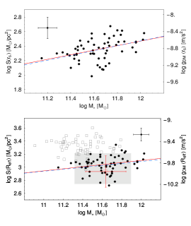
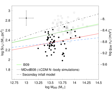
Figure 1: ${\cal{S}}(r_{s})$ and ${\cal{S}}(R_{eff})$ for the NFW + Salpeter model as a function of stellar mass (left panels) and ${\cal{S}}(r_{s})$ vs halo mass $M_{200}$ (right panel), shown as black points. We superimpose the best fit linear relation using the D’ Agostini (2005) (red solid) and direct fit (blue dashed) methods. On the right axes is shown the equivalent acceleration scale $g_{DM}$, defined as in the text and derived by the fit of ${\cal{S}}-g_{DM}$ relation. The black error bars set the median data uncertainties. The results when a Chabrier IMF is used are shown as open boxes. In the left - bottom panel, the median from NRT10 and Tortora et al. (2010) are shown as red symbols and gray region, respectively (in both the cases the $1\sigma$ scatter of the distribution is plotted). In the right panel, we add the B09 best fit linear relation, the secondary - infall model (Boyarsky et al. 2009b) prediction and the results from the $\Lambda$CDM N - body simulation of Macciò, Dutton & van den Bosch (2008).

3.1 The fiducial stellar + DM profile

We have considered four PS + DM models by combining the two halo profiles (Burkert or NFW) with the two IMFs (Chabrier or Salpeter) adopted to set the total stellar mass. We find that all the four models fit remarkably well the lensing and dynamical data with rms deviations $\sim 1\sigma$ and the lens observed values deviating no more than $2\sigma$ from the model ones for most of the bins. On the one hand, such a result ensures us that the estimates of the different quantities entering the scaling relations we are interested in are based on empirically motivated models. On the other hand, this same result tells us that the data we are using are unable to discriminate among different choices. This is an outcome of the limited radial range the data probe. Indeed, given typical values of $R_{E}/R_{eff}$ and $R_{ap}/R_{eff}$, both $M_{E}$ and $\sigma_{ap}$ mainly probe the inner regions of the lenses so that they can provide only weak constraints on the behaviour of the mass profile in the outer DM halo dominated regions.

Although statistically equivalent (as can be quantitatively judged on the basis of the close values of ${\cal{L}}_{max}$ in Tables 1 and 2), the four models may be ranked by examining the constraints on their parameters. Indeed, the values in Table 1 show that the PS + Burkert models fit the data with quite low values of $\Upsilon_{vir}$ thus leading to unexpectedly small virial masses. Roughly averaging the maximum likelihood $\Upsilon_{vir}$ of the different bins, we get $\langle\Upsilon_{vir}\rangle=22\pm 14$ ($12\pm 9$) $M/L_{V,\odot}$ using the Chabrier (Salpeter) IMF. On the contrary, when adopting the NFW profile, we find $\langle\Upsilon_{vir}\rangle=590\pm 210$ ($360\pm 150$) $M/L_{V,\odot}$ for a Chabrier (Salpeter) IMF. Our results from NFW + Salpeter are qualitatively consistent with previous estimates of $\Upsilon_{vir}\sim 200\ \rm M/L_{V,\odot}$ obtained relying on galaxy - galaxy lensing (Guzik & Seljak 2002; Hoekstra et al. 2005) or combining strong and weak lensing and central dynamics (Gavazzi et al. 2007). Therefore, we will consider the NFW + Salpeter as our fiducial model, retaining the other cases just for investigating the dependence of the scaling relations on the halo profiles and IMF adopted. This assumption is also confirmed by recent findings which point to a Salpeter IMF when an uncontracted NFW profile is assumed (Treu et al. 2010; NRT10, Auger et al. 2010a).

The constraints on $(\Upsilon_{vir},\log{\eta_{s}})$ for the four cases considered are summarized in Tables 1 and 2 for Burkert and NFW models respectively. The marginalized constraints on $\Upsilon_{vir}$ show that the NFW + Salpeter model provides reasonable values for the virial $M/L$ ratio in all bins (but the first) thus motivating our choice as a fiducial case. The $68\%$ CL for $\Upsilon_{vir}$ are, however, quite large and asymmetrically extended towards very large values. This can be qualitatively explained noting that the larger is $\Upsilon_{vir}$, the larger is $M_{vir}$ and hence $R_{vir}$. In such a case, $R_{E}/R_{vir}$ and $R_{ap}/R_{vir}$ become quite small such that the data are less and less able to constrain the outer regions. As a consequence, the marginalized likelihood function ${\cal{L}}(\Upsilon_{vir})$ has a long flat tail for large $\Upsilon_{vir}$ thus giving rise to the reported asymmetric errors. A similar effect also explains why the errors on $\log{\eta_{s}}$ are asymmetric and still large. The wide confidence intervals prevent us from quantifying how $\Upsilon_{vir}$ and $\log{\eta_{s}}$ change from one bin to another. Excluding the first bin, characterized by large uncertainties, we find that both $(\Upsilon_{vir},\log{\eta_{s}})$ do not show any significant trend with $L_{V}$.

3.2 DM correlations

We now investigate the relation between the column density ${\cal{S}}(R)=M_{proj}(<R)/\pi R^{2}$, luminosity, stellar and halo mass for the lenses in our sample. The main results of this analysis are shown in Fig. 1. Despite the small mass range probed and the large errors, we find that ${\cal{S}}(r_{s})$ is positively correlated with $L_{V}$, $M_{\star}$ and $M_{200}$, confirming the results in B09. The slope of the correlations may be estimated using the D’ Agostini (2005) fitting method, which takes into account the errors on both variables and the intrinsic scatter $\sigma_{int}$. Concentrating on the trend with stellar mass, for the maximum likelihood parameters, we get

$$\log{{\cal{S}}(r_{s})}=0.29\log{\left(\frac{M_{\star}}{10^{11}\ {\rm M_{\odot}}}\right)}+2.17$$

with an intrinsic scatter $\sigma_{int}=0.01$. Although the results from a direct fit are only slightly different, for completeness we will plot the best fitted relations from both the methods (see Fig. 1). Similar results are found when the column density is fitted as a function of $L_{V}$.

Table 3: Marginalized constraints on the scaling relation parameters for the correlations involving the column density ${\cal{S}}$ assuming the fiducial NFW + Salpeter model. Columns are as follows : 1. correlation id; 2., 3., 4. median value and $68$ confidence ranges for $(\alpha,\beta,\sigma_{int})$, where the linear relation $\log y=\alpha\log x+\beta$ is fitted and $\sigma_{int}$ is the intrisinc scatter. Note that, due to the fitting method, for each value of $(\alpha,\sigma_{int})$, $\beta$ is set by the condition that the likelihood is maximized, in other words we analytically marginalize over $\beta$ when determining the maximum likelihood parameters.

We warn the reader that, in the fit, we use the luminosity $L_{V}$ in units of $10^{11}\ L_{\odot}$ and the stellar (halo) mass in units of $10^{11}(10^{12})\ {\rm M_{\odot}}$ to reduce error covariance.

Id	$(\alpha)_{-1\sigma}^{+1\sigma}$	$(\beta)_{-1\sigma}^{+1\sigma}$	$(\sigma_{int})_{-1\sigma}^{+1\sigma}$
$\log{{\cal{S}}(r_{s})}$ - $\log{L_{V}}$	$0.28_{-0.13}^{+0.13}$	$2.34_{-0.01}^{+0.01}$	$0.037_{-0.027}^{+0.043}$
$\log{{\cal{S}}(r_{s})}$ - $\log{M_{\star}}$	$0.29_{-0.15}^{+0.15}$	$2.16_{-0.09}^{+0.10}$	$0.037_{-0.027}^{+0.043}$
$\log{{\cal{S}}(r_{s})}$ - $\log{M_{200}}$	$0.14_{-0.15}^{+0.15}$	$2.11_{-0.22}^{+0.24}$	$0.040_{-0.029}^{+0.044}$
$\log{{\cal{S}}(R_{eff})}$ - $\log{M_{\star}}$	$0.14_{-0.12}^{+0.12}$	$2.94_{-0.08}^{+0.07}$	$0.057_{-0.032}^{+0.039}$

If we fit the same relation, but replace ${\cal{S}}(r_{s})$ with ${\cal{S}}(R_{eff})$, the trends are shallower, and the zeropoints change too. As shown in Fig. 1, an error weighted average over the galaxies in the sample gives $\langle\log{\cal{S}}(R_{eff})\rangle\sim 3.1$ in agreement, within the scatter, with the median $\log{{\cal{S}}(R_{eff})}\simeq 2.9$ from the local ETG sample of T09 and NRT10 and the results in Tortora et al. (2010) where a different analysis, based on an isothermal profile, is used on the same lens sample. All these results are in agreement with a scenario where ETGs surface from the merging of late - type systems so that, at a fixed radius, their DM content is larger than the one for spirals and dwarves ($\log{{\cal{S}}(R_{eff})}\sim 2\ -\ 2.5$, see NRT10 for further details). Should we use a Chabrier IMF (thus lowering the stellar masses by a factor $\sim 1.8$) we get a larger DM content and ${\cal{S}}(R_{eff})$ which is a constant function of $M_{\star}$ (see open boxes in Fig. 1).

A weaker positive correlation is found when plotting ${\cal{S}}(r_{s})$ vs $M_{200}$, the maximum likelihood fit being

$$\log{{\cal{S}}(r_{s})}=0.16\log{\left(\frac{M_{200}}{10^{12}\ {\rm M_{\odot}}}\right)}+2.11$$

with $\sigma_{int}=0.010$. Our best fit relation is shallower than the B09 one, although the slope is consistent with their one (0.21) within the large error bars. Note that we have here explicitly taken into account the correlated errors on ${\cal{S}}(r_{s})$ and $M_{200}$, while we do not know whether the fitting method adopted by B09 does the same. We therefore cannot exclude that the difference in slope is only an outcome of the use of different algorithms on noisy data. Actually, our ${\cal{S}}(r_{s})$ values are on average smaller than those in B09 (over the same mass range). Our results are also systematically smaller than the estimates from the $\Lambda$CDM N - body simulations of isolated haloes from Macciò, Dutton & van den Bosch (2008) and the predictions from the secondary infall model (B09, Del Popolo 2009). Although a wider mass range has to be probed to infer any definitive answer, we argue that the larger values in the literature are a consequence of neglecting the stellar component. The agreement with B09 would improve if a Chabrier IMF was used (see open boxes in the right panel of Fig. 1) and, as discussed above, the trend would flatten out.

When discussing the results for our reference model, the observed correlations argue against the universality of the column density proposed in D09. It is worth investigating why we and D09 reach completely opposite conclusions. As a first issue, we note that D09 describe the DM halo adopting the Burkert model. Should we use this model to infer ${\cal{S}}(1.6r_{B})$, a Chabrier IMF (which does not strongly differ from the IMFs used in D09), and plot as a function of luminosity to be uniform with them, the best fit relation would have been

$$\log{{\cal{S}}(1.6r_{B})}=0.02\log{\left(\frac{L_{V}}{10^{11}\ {\rm L_{\odot}}}\right)}+2.65$$

with $\sigma_{int}=0.15$. In such a case, within a very good approximation, we can assume ${\cal{S}}(1.6r_{B})$ is indeed constant with $L_{V}$. An error weighted average of the sample values gives $\langle\log{{\cal{S}}(1.6r_{B})}\rangle=3.07\pm 0.02\pm 0.20$, where here and in following similar estimates, the first error is the statistical uncertainty and the second one the rms around the mean. Taken at face value, this estimate is significantly larger than the D09 one (similarly to what was found when discussing the comparison among the ${\cal{S}}(R_{eff})$ values for ETGs and spirals), even if it is marginally within $2\sigma_{rms}$. However, as discussed above, the slope of the ${\cal{S}}_{B}(1.6r_{B})$ - $L_{V}$ relation is strongly model dependent. Indeed, changing to a Salpeter IMF, we find ${\cal{S}}_{B}(1.6r_{B})\propto L_{V}^{0.20}$ thus arguing in favour of non universality. Actually, the Burkert model is likely to be unable to fit the data for ETGs with reasonable values of $\Upsilon_{vir}$ so that one should rely on the NFW + Salpeter results to thus conclude that the column density ${\cal{S}}$ depends on mass for intermediate redshift ETGs. Investigating the reasons why NFW models are preferred over Burkert ones for ETGs, while the opposite is true for spirals can provide important constraints on galaxy formation scenarios, but it is outside our scope here.

Motivated by the D09 findings on the universality of $\rho_{B}r_{B}$ and noting that the DM Newtonian acceleration, $g_{DM}(r)=GM_{DM}(r)/r^{2}$, is proportional to $\rho_{B}r_{B}$ for a Burkert model, G09 have recast the D09 results in terms of a constancy of $g_{DM}(r_{B})$. Then they extended this result showing that also the stellar acceleration, $g_{\star}(r)=GM_{\star}(r)/r^{2}$ at $r_{B}$ is a universal quantity. Using their same Burkert model and a Chabrier IMF, we indeed find that $g_{DM}(r_{B})$ is roughly constant with $L_{V}$, with an error weighted value $\langle\log{g_{DM}(r_{B})}\rangle=-8.89\pm 0.02\pm 0.20$, in satisfactory agreement with the G09 result ($\log{g_{DM}(r_{B})}\simeq-8.5$). Having said that, we find that $g_{\star}(r_{B})$ is not constant, the best fit relation predicting $g_{\star}(r_{B})\propto L_{V}^{-0.21}$. We stress, however, that the situation is completely reversed if we use a Salpeter IMF giving $g_{DM}(r_{B})\propto L_{V}^{0.20}$ and $g_{\star}(r_{B})\propto L_{V}^{-0.01}$, so that drawing a definitive answer on which quantity is universal is an ambiguous task. Whatever is the correct IMF, we can nevertheless safely conclude that the DM and stellar Newtonian accelerations cannot both be universal quantities, in contrast with the claim in G09. Moreover, should the IMF be universal and intermediate between Chabrier and Salpeter, one could argue that neither $g_{DM}(r_{B})$ and $g_{\star}(r_{B})$ are universal quantities.

Table 4: Marginalized constraints on the scaling relation parameters for the correlations $\log{g_{DM}(R_{eff})}$ - $\log{L_{V}}$ (upper part) and $\log{g_{\star}(R_{eff})}$ - $\log{L_{V}}$ (lower part) with the accelerations in ${\rm m/s^{2}}$ and the luminosity in units of $10^{11}\ {\rm L_{\odot}}$. Columns are as follows : 1. model id, 2., 3., 4. median value and $68$ per cent confidence ranges for $(\alpha,\beta,\sigma_{int})$. The model ids are BSC for Burkert + Chabrier, BSS for Burkert + Salpeter, NSC for NFW + Chabrier, NSS for NFW + Salpeter. Note that, since $g_{\star}(R_{eff})$ refers to stellar quantities only, the correlations involving this quantity are independent on the halo model.

Model Id	$(\alpha)_{-1\sigma}^{+1\sigma}$	$(\beta)_{-1\sigma}^{+1\sigma}$	$(\sigma_{int})_{-1\sigma}^{+1\sigma}$
BSC	$-0.155_{-0.145}^{+0.145}$	$-9.090_{-0.003}^{+0.003}$	$0.175_{-0.019}^{+0.023}$
BSS	$-0.004_{-0.142}^{+0.144}$	$-9.322_{-0.002}^{+0.004}$	$0.156_{-0.029}^{+0.033}$
NSC	$0.088_{-0.111}^{+0.111}$	$-9.526_{-0.004}^{+0.004}$	$0.066_{-0.035}^{+0.043}$
NSS	$0.245_{-0.125}^{+0.126}$	$-9.841_{-0.006}^{+0.007}$	$0.040_{-0.028}^{+0.043}$
NSC	$-0.461_{-0.168}^{+0.170}$	$-9.649_{-0.005}^{+0.004}$	$0.178_{-0.022}^{+0.028}$
NSS	$-0.461_{-0.168}^{+0.170}$	$-9.403_{-0.005}^{+0.004}$	$0.178_{-0.022}^{+0.028}$

As already discussed, our fiducial model is the NFW + Salpeter so that it is preferable to use this model when investigating whether the Newtonian accelerations are constant or not. Moreover, rather than using the halo characteristic radius (which refers to a different mass content depending on the model), we will discuss the results at $R_{eff}$ thus referring to the better constrained inner regions. For the fiducial model, we find $\log{g_{DM}(R_{eff})}\propto 0.26\log{L_{V}}$ thus arguing against the universality of this quantity. However, as can be seen in Table 4, the slope of the $g_{DM}(R_{eff})$ - $L_{V}$ correlation is strongly model dependent with values indicating either an increasing behaviour (for NFW models), a flat one (for Burkert + Salpeter) or a decreasing one (for Burkert + Chabrier). These trends are expected from the analysis of column density made above. On the contrary, the scaling of $g_{\star}(R_{eff})$ does not depend on the halo model because its value is estimated from stellar quantities only, while the effect of the IMF is simply a systematic rescaling due to the higher stellar masses for the Salpeter case. Although the slope in Table 4 points towards a significative decrease with the luminosity, it is worth stressing that assuming a constant value $\langle\log{g_{\star}(R_{eff})}\rangle=-9.403\pm 0.01\pm 0.20$ (for a Salpeter IMF) provides a similarly good fit so that we can not draw a definitive answer.

Any correlation between a DM quantity and a stellar one may be the outcome of a hidden interaction between the two galactic components. In particular, for the Newtonian accelerations, because of their definition, it is straightforward to show that $g_{DM}(R_{eff})=GM_{DM}(R_{eff})/R_{eff}^{2}=M_{DM}(R_{eff})/M_{eff}\times g_{\star}(R_{eff})$ with $M_{eff}=M_{\star}(R_{eff})$ so that one can look for a correlation between these two quantities. For the NFW + Salpeter model, we indeed get :

$$\log{g_{DM}(R_{eff})}=0.21\log{g_{\star}(R_{eff})}-7.89\ .$$

with $\sigma_{int}=0.018$, the marginalized constraints being :

$$\alpha=0.20_{-0.13}^{+0.13}\ \ ,\ \ \beta=-7.90_{-1.28}^{+1.13}\ \ ,\ \ \sigma_{int}=0.042_{-0.030}^{+0.043}\ \ .$$

Actually, we can recast the above relation in a different way. From the definitions of $g_{DM}(R_{eff})$ and $g_{\star}(R_{eff})$ and the assumption $\log{g_{DM}(R_{eff})}\propto\alpha\log{g_{\star}(R_{eff})}$, one easily gets :

$$\log{M_{DM}(R_{eff})}\propto 2(1-\alpha)\log{R_{eff}}+\alpha\log{M_{eff}}$$

so that we fit a loglinear relation

$$\log{M_{DM}(R_{eff})}=\alpha_{M}\log{R_{eff}}+\beta_{M}\log{M_{eff}}+\gamma_{M}\ .$$

For the best fit relation, we find $(1.46,0.60,2.79)$ with $\sigma_{int}=0.006$, while the marginalized constraints (median and $68\%$ CL) read

$$\alpha_{M}=1.47_{-0.26}^{+0.25}\ \ ,\ \ \beta_{M}=0.61_{-0.21}^{+0.22}\ \ ,$$

$$\gamma_{M}=2.54_{-0.26}^{+0.41}\ \ ,\ \ \sigma_{int}=0.029_{-0.020}^{+0.033}\ .$$

For $\alpha=0.21$, we expect $\alpha_{M}\simeq 1.58$ in agreement with our estimate. On the contrary, $\beta_{M}$ is significantly larger than $\alpha$ possibly indicating that the ratio $g_{DM}(R_{eff})/g_{\star}(R_{eff})$ depends on the stellar mass more than expected. However, because of the correlation between $\beta_{M}$ and $\sigma_{int}$ induced by the fit, a wrong estimate of the intrinsic scatter may induce a bias in the best fit $\beta_{M}$. Since the error bars are quite large, determining $\sigma_{int}$ is a difficult task as can also be understood noting that the best fit $\sigma_{int}$ is formally outside the marginalized $68\%$ confidence range (but within the $95\%$ one). Nevertheless, the small value of the rms of the residuals ($\sigma_{rms}=0.12$) is strong evidence in favour of a very tight correlation. We also stress that this scaling relation (although with different coefficients) still holds if we change the IMF or the halo model. Interestingly, this correlation is pretty similar to the luminosity and mass FP discussed in Bolton et al. (2007) and Hyde & Bernardi (2009), with the total $M/L$ ratio found to depend less on the stellar mass density than on the effective radius.

An alternative way to look for the correlation between the stellar and DM mass at $R_{eff}$ may be provided by the DM mass fraction, $f_{DM}(R_{eff})=M_{DM}(R_{eff})/[M_{\star}(R_{eff})+M_{DM}(R_{eff})]$. Since $M_{DM}(R_{eff})$ and $M_{\star}(R_{eff})$ are correlated, we expect to find a similar correlation between $f_{DM}(R_{eff})$ and mass proxies, such as $M_{\star}$ and $L_{V}$ (Cappellari et al. 2006, Bolton et al. 2007, Hyde & Bernardi 2009, T09, Auger et al. 2010b). We indeed find

$$\log{f_{DM}(R_{eff})}=0.49\log{\left(\frac{M_{\star}}{10^{11}\ {\rm L_{\odot}}}\right)}-0.86\ ,$$

$$\log{f_{DM}(R_{eff})}=0.51\log{\left(\frac{L_{V}}{10^{11}\ {\rm L_{\odot}}}\right)}-0.56\ ,$$

with $\sigma_{int}=0.03$ (0.02) and $\sigma_{rms}=0.13$ (0.12) for the first (second) case. The marginalized constraints for the $f_{DM}$ - $M_{\star}$ relation are :

$$\alpha=0.48_{-0.11}^{+0.11}\ ,\ \beta=-0.86_{-0.08}^{+0.08}\ ,\ \sigma_{int}=0.049_{-0.032}^{+0.041}\ ,$$

while for the $f_{DM}$ - $L_{V}$ we find :

$$\alpha=0.51_{-0.09}^{+0.09}\ ,\ \beta=-0.57_{-0.01}^{+0.01}\ ,\ \sigma_{int}=0.028_{-0.021}^{+0.038}\ ,$$

The large error bars on the individual points likely make the estimate of $\sigma_{int}$ biased, but we nevertheless find clear evidence for a DM content increasing with both $M_{\star}$ and $L_{V}$. Both these correlations are in very good agreement with what is found in T09 for local ETGs for high luminosity systems ($\log{L_{B}}\geq 10.4$), notwithstanding the different models adopted (NFW halo and Sersic stellar profile here vs a full isothermal model in T09). However, the slopes we find are strongly dependent on the model assumptions. Should we use the same NFW model, but the Chabrier IMF, we get $f_{DM}(R_{eff})\propto L_{V}^{0.20}$ and $f_{DM}(R_{eff})\propto M_{\star}^{0.16}$, which are fully consistent with the results we have obtained in Cardone et al. (2009), where a general galaxy model has been fitted to a subsample of SLACS lenses.

4 Conclusions

Much attention has recently been dedicated to investigating whether some correlations can be found among DM quantities and the stellar ones with contrasting results pointing towards a universal DM column density ${\cal{S}}$ (D09, G09) or its variation with halo mass $M_{200}$ (B09) and luminosity $M_{\star}$ (T09, NRT10, Auger et al. 2010a). Here we have addressed this controversy using a sample of intermediate redshift ETGs using the available data on both the projected mass within the Einstein radius and the aperture velocity dispersion to fit four different stellar + DM halo models. Motivated by recent findings in the literature (Treu et al. 2010, NRT10) and the analysis of the virial $M/L$ ratio, we have finally chosen a NFW DM halo and a Salpeter IMF which we have then used as a reference case for investigating the scaling relations of interest.

Contrary to D09, we find that the column density ${\cal{S}}$, evaluated at both the halo characteristic radius $r_{s}$ or the stellar effective radius $R_{eff}$ is not a universal quantity, but rather correlates with the luminosity $L_{V}$ and the stellar and halo masses $M_{\star}$ and $M_{200}$. Although the slopes of these correlations depend on the halo model and IMF, assuming our reference model, the ${\cal{S}}(r_{s})$ - $M_{200}$ relation we find agrees with the B09 one, with a rather similar slope (0.19 vs 0.21), but a smaller zeropoint. As a consequence, our ${\cal{S}}(r_{s})$ values are smaller than the B09 ones, but also smaller than those predicted on the basis of a secondary infall model (B09, Del Popolo 2009) and $\Lambda CDM$ N - body simulations (Macciò, Dutton & van den Bosch, 2008). We argue that this discrepancy is expected considering that these studies do not add a stellar component to the galaxy model, while here we take this explicitly into account thus decreasing the DM content. We have also found that the ensemble average column density in the central regions is systematically larger than the one in spiral galaxies in agreement with, e.g., NRT10. This is consistent with mass accretion in more massive haloes due to merging of late - type systems. As an interesting new result, we have shown that a very tight loglinear relation among $M_{DM}(R_{eff})$, $R_{eff}$ and $M_{eff}$ can be found leading to a DM mass fraction which positively correlates with both the stellar luminosity and mass (Cappellari et al. 2006, Bolton et al. 2007, Hyde & Bernardi 2009, T09).

The limited mass and luminosity range probed and the large errors on the different quantities involved prevent us from drawing a definitive answer on the slope and normalization of the above scaling relations. Moreover, a larger dataset should also allow us to make a more detailed investigation of the impact of halo profiles and IMF assumptions. Should these further tests confirm our results, DM scaling relations can provide a valuable tool in understanding the physical processes which drive galaxy formation and evolution.

References

• Auger et al. (2009) Auger, M.W., Treu, T., Bolton, A.S., Gavazzi, R., Koopmans, L.V.E., Marshall, P.J., Bundy, K., Moustakas, L.A. 2009, ApJ, 705, 1099
• Auger et al. (2010a) Auger, M.W., Treu, T., Gavazzi, R., Bolton, A.S., Koopmans, L.V.E., Marshall, P.J. 2010a, preprint arXivโ€‰:1007.2409
• Auger et al. (2010b) Auger, M.W., Treu, T., Bolton, A.S., Gavazzi, R., Koopmans, L.V.E., Marshall, P.J., Moustakas, L.A., Burles, S. 2010b, preprint arXivโ€‰:1007.2880
• Bartelmann (1996) Bartelmann, M. 1996, A&A, 313, 697
• Bertschinger (1998) Bertschinger, E. 1998, ARA&A, 36, 599
• Bolton et al. (2007) Bolton A.S. 2007, ApJ, 665, 105
• Boyarsky et al. (2009a) Boyarsky, A., Ruchayskiy, O., Iakubovskyi, D., Macciรฒ, A.V., Malyshev, D. 2009a, arXivโ€‰:โ€‰0911.1774 (B09)
• Boyarsky et al. (2009b) Boyarsky, A., Neronov, A., Ruchayskiy, O., Tkachev, I. 2009b, arXivโ€‰:โ€‰0911.3369
• Bryan & Norman (1998) Bryan, G.L., Norman, M.L. 1998, ApJ, 495, 80
• Burkert (1995) Burkert, A. 1995, ApJ, 447, L25
• Cappellari et al. (2006) Cappellari M. et al. 2006, MNRAS, 366, 1126
• Cardone et al. (2009) Cardone, V.F., Tortora, C., Molinaro, R., Salzano, V. 2009, A&A, 504, 769
• Carroll et al. (1992) Carroll, S.M., Press, W.H., Turner, E.L. 1992, ARA&A, 30, 499
• Chabrier (2001) Chabrier, G. 2001, ApJ, 554, 1274
• Dโ€™ Agostini (2004) Dโ€™ Agostini, G. 2004, arXivโ€‰: physics/0403086
• Dโ€™ Agostini (2005) Dโ€™ Agostini, G. 2005, arXivโ€‰: physics/0511182
• de Blok (2009) de Blok, W.J.G. 2009, arXivโ€‰:0910.3538
• Del Popolo (2009) Del Popolo, A. 2009, ApJ 698, 2093
• Donato et al. (2009) Donato, F., Gentile, G., Salucci, P., Frigerio Martins, C., Wilkinson, M.I., Gilmore, G., Grebel, E.K., Koch, A., Wyse, R. 2009, MNRAS, 397, 1169 (D09)
• Gavazzi et al. (2007) Gavazzi, R., Treu, T., Rhodes, J.D., Koopmans, L.V.E., Bolton, A.S., Burles, S., Massey, R.J., Moustakas, L.A. 2007, ApJ, 667, 176
• Gentile et al. (2009) Gentile, G., Famaey, B., Zhao, H.S., Salucci, P. 2009, Nature, 461, 627 (G09)
• Graves & Faber (2010) Graves, G.J., Faber, S.M. 2010, preprint arXivโ€‰:1005.0014
• Guzik & Seljak (2002) Guzik, J., Seljak, U. 2002, MNRAS, 335, 311
• Hyde & Bernardi (2009) Hyde J.B. & Bernardi M. 2009, MNRAS, 396, 1171
• Hoekstra et al. (2005) Hoekstra, H., Hsieh, B.C., Yee, H.K.C., Lin, H., Gladders, M.D. 2005, ApJ, 635, 73
• Komatsu et al. (2009) Komatsu, E., Dunkley, J., Nolta, M.R., Bennett, C.L., Gold, B. et al. 2009, ApJS, 180, 330
• Lampteil et al. (2009) Lampeitl, H., Nichol, R.C., Seo, H.J., Giannantonio, T., Shapiro, C. et al. 2010, MNRAS, 401, 2331
• Macciรฒ, Dutton & van den Bosch (2008) Macciรฒ, A.V., Dutton, A.A., van den Bosch, F.C. 2008, MNRAS, 391, 1940
• Mamon & Lokas (2005) Mamon, G., Lokas, E. 2005, MNRAS, 363, 705
• Marquez et al. (2001) Marquez, I., Lima Neto, G.B., Capelato, H., Durret, F., Lanzoni, B., Gerbal, D. 2001, A&A, 379, 767
• Napolitano, Romanowsky & Tortora (2010) Napolitano, N.R., Romanowsky A.J. & Tortora, C. 2010, arXiv:1003.1716 (NRT10)
• Navarro et al. (1997) Navarro, J.F., Frenk, C.S., White, S.D.M. 1997, ApJ, 490, 493
• Park & Ferguson (2003) Park, Y., Ferguson, H.C. 2003, ApJ, 589, L65
• Percival et al. (2009) Percival, W.J., Reid, B.A., Eisenstein, D.J., Bachall. N.A., Budavari, T. et al. 2010, MNRAS, 401, 2148
• Prugniel & Simien (1997) Prugniel, Ph., Simien, F. 1997, A&A, 321, 111
• Salpeter (1955) Salpeter, E.E. 1955 ApJ, 121, 161
• S$\rm\acute{e}$rsic (1968) S$\rm\acute{e}$rsic, J.L. 1968, Atlas de Galaxies Australes, Observatorio Astronomico de Cordoba
• Thomas et al. (2009) Thomas J., Saglia R. P., Bender R., Thomas D., Gebhardt K., Magorrian J., Corsini E. M., Wegner G., 2009, ApJ, 691, 770
• Tortora et al. (2009) Tortora, C., Napolitano, N.R., Romanowsky, A.J., Capaccioli, M., Covone, G. 2009, MNRAS, 396, 1132 (T09)
• Tortora et al. (2010) Tortora, C. et al. 2010, ApJ submitted
• Treu et al. (2010) Treu, T., Auger, M. W., Koopmans, L. V. E., Gavazzi, R., Marshall, P. J. & Bolton, A. S. 2010, ApJ, 709, 119