On smoothness of Black Saturns

Abstract

We prove smoothness of the domain of outer communications (d.o.c.) of the Black Saturn solutions of Elvang and Figueras. We show that the metric on the d.o.c. extends smoothly across two disjoint event horizons with topology $\mathbb{R}\times S^{3}$ and $\mathbb{R}\times S^{1}\times S^{2}$. We establish stable causality of the d.o.c. when the Komar angular momentum of the spherical component of the horizon vanishes, and present numerical evidence for stable causality in general.

1 Introduction

In [4], Elvang and Figueras introduced a family of vacuum five-dimensional asymptotically flat metrics, to be found in Appendix A.1, and presented evidence that these metrics describe two-component black holes, with Killing horizon topology $\mathbb{R}\times\big{(}(S^{1}\times S^{2})\cup S^{3})\big{)}$. In this paper we construct extensions of the metrics across Killing horizons, with the Killing horizon becoming an event horizon in the extended space-time. Now, it is by no means clear that those metrics have no singularities within their domains of outer communications (d.o.c.), and the main purpose of this work is to establish this for non-extreme configurations. Again, it is by no means clear that the d.o.c.’s of the solutions are well behaved causally. We prove that those d.o.c.’s are stably causal when the parameter $c_{2}$ vanishes (this condition is equivalent to the vanishing of the Komar angular momentum of the spherical component of the horizon, compare [4, Equation (3.39)]), and present numerical evidence suggesting that this is true in general.

Given the analytical and numerical evidence presented here, it appears that the Black Saturn metrics describe indeed well behaved black hole space-times within the whole range of parameters given by Elvang and Figueras, except possibly for the degenerate cases when some parameters $a_{i}$ coalesce, a study of which is left for future work. In particular we have rigorously established that the Black Saturn metrics with $c_{2}=0$ and with distinct $a_{i}$’s have a reasonably well behaved neighbourhood of the d.o.c. Our reticence here is related to the fact that we have not proved global hyperbolicity of the d.o.c., which is often viewed as a desirable property of the domains of outer communications of well behaved black holes. In view of our experience with the Emperan-Reall metrics [2], the proof of global hyperbolicity (likely to be true) appears to be a difficult task.

We use the notation of [4], and throughout this paper we assume that the parameters $a_{i}$ occurring in the metric are pairwise distinct, $a_{i}\neq a_{j}$ for $i\neq j$.

2 Regularity at $z=a_{1}$, $\rho=0$, and the choice of $c_{1}$

We consider the metric coefficient $g_{tt}$ on the set $\{\rho=0,z<a_{1}\}$. A Mathematica calculation shows that $g_{tt}$ is a rational function with denominator given by

$$-\left(2(a_{3}-a_{1})(a_{2}-a_{4})+(a_{5}-a_{1})c_{1}c_{2}\right)^{2}(z-a_{1})(z-a_{2})(z-a_{4})\;,$$ (2.1)

which clearly vanishes as $z$ approaches $a_{1}$ from below (we will see in Section 4 that the first multiplicative factor is non-zero with our choices of constants). On the other hand, its numerator has the following limit as $z\to a_{1}$,

$$(a_{2}-a_{1})^{2}(a_{3}-a_{1})(a_{5}-a_{1})\left(2(a_{3}-a_{1})(a_{4}-a_{1})-(a_{5}-a_{1})c_{1}^{2}\right)c_{2}^{2}\;,$$ (2.2)

which is non-zero unless $c_{2}$ vanishes or $c_{1}$ is chosen to make the before-last factor vanish:

$$c_{1}=\pm\sqrt{\frac{2(a_{3}-a_{1})(a_{4}-a_{1})}{a_{5}-a_{1}}}\neq 0\;.$$ (2.3)

This coincides with Equation (3.7) of [4].

By inspection, one finds that the metric is invariant under the transformation

$$(c_{1},c_{2},\psi)\mapsto(-c_{1},-c_{2},-\psi)\;.$$

Thus, an overall change of sign $(c_{1},c_{2})\mapsto(-c_{1},-c_{2})$ can be implemented by a change of orientation of the angle $\psi$. Hence, to understand the global structure of the associated space-time, it suffices to consider the case

$$c_{1}>0\;;$$

this will be assumed throughout the paper from now on.

If (2.3) does not hold, the Lorentzian norm squared $g_{tt}=g(\partial_{t},\partial_{t})$ of the Killing vector $\partial_{t}$ is unbounded as one approaches $a_{1}$; a well known argument shows that this leads to a geometric singularity.

We show in Section 5.8.1 that the choice (2.3) is necessary for regularity of the metric regardless of whether or not $c_{2}=0$: without this choice, $g_{\psi\psi}$ would be unbounded near $a_{1}$, leading to a geometric singularity as before.

With the choice (2.3) of $c_{1}$, or with $c_{2}=0$, the point $\alpha_{1}:=(\rho=0,z=a_{1})$ in the quotient of the space-time by the action of the isometry group becomes a ghost point, in the sense that it has no natural geometric interpretation, such as a fixed point of the action, or the end-point of an event horizon. Now, the functions

$$R_{i}:=\sqrt{\rho^{2}+(z-a_{i})^{2}}$$

are not differentiable at $\rho=0,z=a_{i}$. So, a generic function of $R_{1}$ will have some derivatives blowing up at $\rho=0,z=a_{1}$. However, this will not happen for functions which are smooth functions of $R_{1}^{2}$. It came as a major surprise to us that the choice of $c_{1}$ above, determined by requiring boundedness of $g_{tt}$ on the axis near $a_{1}$, also leads to smoothness of all metric functions near $z=a_{1}$. It turns out that there is a general mechanism which guarantees that; this will be discussed elsewhere [3].

To establish that the metric is indeed smooth near the ghost point $\alpha_{1}$, we start with

$$g_{tt}=-\frac{H_{y}}{H_{x}}=-\frac{FH_{y}}{FH_{x}}=:\Phi(\mu_{1},\mu_{A},c_{1},c_{2},\rho^{2})\;,$$

where $A$ runs from two to five. $\Phi$ is a rational function of its arguments, and hence a rational function of $R_{1}$. So $g_{tt}$ will be a smooth function of $R_{1}^{2}$ near $R_{1}=0$ if and only if $\Phi$ is even in $R_{1}$:

$$\Phi(R_{1}-(z-a_{1}),\mu_{A},c_{1},c_{2},\rho^{2})=\Phi(-R_{1}-(z-a_{1}),\mu_{A},c_{1},c_{2},\rho^{2})\;,$$ (2.4)

assuming moreover that the right value of $c_{1}$ has been inserted. (We emphasise that neither $FH_{x}$ or $FH_{y}$ are even in $R_{1}^{2}$, so there is a non-trivial factorisation involved; moreover $g_{tt}$ is not even in $R_{1}$ for arbitrary values of the $c_{i}$’s, as is seen by setting $c_{1}=c_{2}=0$.) Now, there is little hope of checking this identity by hand after all functions have been expressed in terms of $\rho$, $z$, and the $a_{i}$’s, and we have not been able to coerce Mathematica to deliver the required result in this way either. Instead, to avoid introducing new functions or parameters into $\Phi$, we first note that

$$-R_{1}-(z-a_{1})=-\frac{\rho^{2}}{\mu_{1}}\;,$$

and so (2.4) reads

$$\Phi(\mu_{1},\mu_{A},c_{1},c_{2},\rho^{2})=\Phi\big{(}-\frac{\rho^{2}}{\mu_{1}},\mu_{A},c_{1},c_{2},\rho^{2}\big{)}\;.$$

From the explicit form of the functions $FH_{x}$ and $FH_{y}$ we can write

$$\Phi(\mu_{1},\mu_{A},c_{1},c_{2})-\Phi\big{(}-\frac{\rho^{2}}{\mu_{1}},\mu_{A},c_{1},c_{2}\big{)}=\frac{\sum_{i=0}^{4}\Phi_{i}(c_{1}c_{2})^{i}}{G}\;,$$

where the $\Phi_{i}$’s are polynomials in $c_{1}^{2}$, $\mu_{i}$ and $\rho^{2}$, and $G$ is a polynomial in $\mu_{i}$, $c_{1}$, $c_{2}$ and $\rho^{2}$. One then checks with Mathematica that each of the coefficients $\Phi_{i}$ has a multiplicative factor that vanishes after applying the identity (5.1) below to replace each occurrence of $c_{1}^{2}$ in terms of the $\mu_{i}$’s:

$$c_{1}^{2}=\frac{(-\mu_{1}+\mu_{3})(-\mu_{1}+\mu_{4})\mu_{5}(\mu_{1}\mu_{3}+\rho^{2})(\mu_{1}\mu_{4}+\rho^{2})}{\mu_{1}\mu_{3}\mu_{4}(-\mu_{1}+\mu_{5})(\mu_{1}\mu_{5}+\rho^{2})}\;.$$

It is rather fortunate that each of those coefficients has a vanishing factor, as we have not been able to convince Mathematica to carry out a brute-force calculation on all coefficients at once.

An identical analysis applies to $g_{\rho\rho}=g_{zz}$ and $\omega_{\psi}/H_{y}$; regularity of $g_{\psi\psi}$ immediately follows; there is nothing to do for $g_{\varphi\varphi}$. Before doing these calculation, care has to be taken to eliminate, with the right signs, all square roots of squares that appear in the definition of $\omega_{\psi}$.

3 Asymptotics at infinity: the choice of $q$ and $k$

We wish to check that the Black Saturn metric is asymptotically flat. As a guiding principle, the Minkowski metric on $\mathbb{R}^{5}$ is written in coordinates adapted to ${\bf U}(1)\times{\bf U}(1)$ symmetry as

$$\eta = -dt^{2}+d\tilde{x}^{2}+d{\tilde{y}}^{2}+d{\hat{x}}^{2}+d{\hat{y}}^{2}$$ (3.1)

$$= -dt^{2}+d{\tilde{\rho}}^{2}+{\tilde{\rho}}^{2}d\psi^{2}+d\hat{\rho}^{2}+\hat{\rho}^{2}d\varphi^{2}\;,$$

with

$$(\tilde{x},{\tilde{y}})={\tilde{\rho}}(\cos\psi,\sin\psi)\;,\quad({\hat{x}},{\hat{y}})=\hat{\rho}(\cos\varphi,\sin\varphi)\;.$$

Introducing $\rho$ and $\theta$ as polar coordinates in the $(\hat{\rho},{\tilde{\rho}})$ plane,

$$(\hat{\rho},{\tilde{\rho}})=r(\cos\theta,\sin\theta)\;,$$

the metric (3.1) becomes

$$\eta=-dt^{2}+dr^{2}+r^{2}d\theta^{2}+r^{2}\sin^{2}\theta\,d\psi^{2}+r^{2}\cos^{2}\theta\,d\varphi^{2}\;.$$ (3.2)

Note that $\theta\in[0,\pi/2]$ since both ${\tilde{\rho}}$ and $\hat{\rho}$ are positive in our range of interest.

As outlined by Elvang and Figueras in [4], relating the $(\rho,z,\psi,\varphi)$ coordinates of the Black Saturn metric to the $(r,\theta,\psi,\varphi)$ coordinates of (3.2) via the formulae

$$\rho=\frac{1}{2}r^{2}\sin 2\theta\;,\quad z=\frac{1}{2}r^{2}\cos 2\theta\;,\quad\theta\in\left[0,\frac{\pi}{2}\right]\;,$$ (3.3)

should lead to a metric which is asymptotically flat. Under (3.3) the metric (3.2) becomes

$$\eta=-dt^{2}+r^{-2}(d\rho^{2}+dz^{2})+r^{2}\sin^{2}\theta\,d\psi^{2}+r^{2}\cos^{2}\theta\,d\varphi^{2}\;,$$ (3.4)

so that in such coordinates a set of necessary conditions for asymptotic flatness reads

$$g_{tt}\to-1\;,\ r^{-1}\sin^{-1}\theta\,g_{t\psi}\to 0\;,\$$ (3.5)

$$r^{2}g_{\rho\rho}=r^{2}g_{zz}\to 1\;,\ r^{-2}\sin^{-2}\theta\,g_{\psi\psi}\to 1\;,\ r^{-2}\cos^{-2}\theta\,g_{\varphi\varphi}\to 1\;,$$ (3.6)

when $r$ tends to infinity. One also needs to check that all metric components are suitably behaved when transformed to the coordinates $(\tilde{x},{\tilde{y}},{\hat{x}},{\hat{y}})$ above. Finally, each derivative of any metric components should decay one order faster than the preceding one.

We start by noting that

$$z=\frac{1}{2}r^{2}(\cos^{2}\theta-\sin^{2}\theta)=\frac{1}{2}(\hat{\rho}^{2}-{\tilde{\rho}}^{2})$$

which is a smooth function of $(\tilde{x},{\tilde{y}},{\hat{x}},{\hat{y}})$. On the other hand,

$$\rho=r^{2}\sin\theta\,\cos\theta=\hat{\rho}{\tilde{\rho}}$$

is not smooth, but its square is. This implies that all the functions appearing in the metric are smooth functions of $(\tilde{x},{\tilde{y}},{\hat{x}},{\hat{y}})$, except perhaps at zeros of the functions $R_{i}$ and of the denominators; the former clearly do not occur at sufficiently large distances, while the denominators have no zeros for $\rho>0$ by Section 5.3, and at $\rho=0$ away from the points $a_{i}$ by Sections 5.4 and 5.8.1.

To control the asymptotics we note that $\mu_{i}=O(r^{2})$, but more precise control is needed. Setting $R^{2}:=\rho^{2}+z^{2}=r^{4}/4$, a Taylor expansion within the square root gives

$$\mu_{i} = \sqrt{\rho^{2}+(z-a_{i})^{2}}-(z-a_{i})$$

$$= R\sqrt{1-\frac{2za_{i}-a_{i}^{2}}{R^{2}}}-(z-{a_{i}})$$

$$= \big{(}r^{2}+2a_{i}+2\frac{a_{i}^{2}}{r^{2}}(1+\cos 2\theta)\big{)}\sin^{2}\theta+O(r^{-4})$$

$$= (r^{2}+2a_{i})\sin^{2}\theta+O(r^{-2})\;.$$

For $z\leq 0$ this can be rewritten as

$$\mu_{i}=(r^{2}+2a_{i}+O(r^{-2}))\sin^{2}\theta\;.$$ (3.7)

To see that the last equation remains valid for $z\geq 0$ we write instead

$$\mu_{i} = \frac{\rho^{2}}{\sqrt{\rho^{2}+(z-a_{i})^{2}}+(z-a_{i})}$$

$$= \frac{R^{2}\sin^{2}2\theta}{R\sqrt{1-\frac{2za_{i}-a_{i}^{2}}{R^{2}}}+(z-{a_{i}})}$$

$$= \frac{R\sin^{2}2\theta}{1-\frac{za_{i}}{R^{2}}+\frac{z}{R}-\frac{a_{i}}{R}+O(R^{-2})}$$

$$= \frac{R\sin^{2}2\theta}{(1+\frac{z}{R})(1-\frac{a_{i}}{R}+O(R^{-2}))}$$

$$= \big{(}R+a_{i}+O(R^{-1})\big{)}\frac{\sin^{2}2\theta}{1+\cos 2\theta}\;,$$

and we have recovered (3.7) for all $z$, for $r$ large, uniformly in $\theta$.

The above shows that $\mu_{i}-\mu_{j}=O(1)$ for large $r$; in fact, for $i\neq j$,

$$\mu_{i}-\mu_{j}=\big{(}2(a_{i}-a_{j})+O(r^{-2})\big{)}\sin^{2}\theta\;.$$

Keeping in mind that

$$\rho^{2}+\mu_{i}\mu_{j}\approx r^{4}\sin^{2}\theta\;,$$

where we use $f\approx g$ to denote that $C^{-1}\leq f/g\leq C$ for large $r$, for some positive constant $C$, we are led to the following uniform estimates

$$M_{0}\approx r^{30}\sin^{26}\theta\;,$$

$$M_{1}\approx r^{24}\sin^{28}\theta\sin^{2}2\theta\;,\ M_{1}\frac{\rho^{2}}{\mu_{1}\mu_{2}}\approx r^{24}\sin^{24}\theta\sin^{4}2\theta\;,$$

$$M_{2}\approx r^{28}\sin^{24}\theta\sin^{2}2\theta\;,\ M_{2}\frac{\mu_{1}\mu_{2}}{\rho^{2}}\approx r^{28}\sin^{28}\theta\;,\$$

$$M_{3}\approx r^{30}\sin^{26}\theta\ \;,\ M_{4}\approx r^{30}\sin^{26}\theta\;,$$

$$F\approx r^{48}\sin^{34}\theta\;,$$

$$\displaystyle G_{x}=\frac{r^{2}\sin^{2}2\theta}{4\sin^{2}\theta}\big{(}1+O(r^{-2})\big{)}\approx r^{2}\cos^{2}\theta\;,$$

$$P=(\mu_{3}\,\mu_{4}+\rho^{2})^{2}(\mu_{1}\,\mu_{5}+\rho^{2})(\mu_{4}\,\mu_{5}+\rho^{2})\approx r^{16}\sin^{8}\theta\,.$$

This shows that, for large $r$,

$$H_{x} = F^{-1}\,\bigg{[}\underbrace{M_{0}+c_{1}\,c_{2}\,M_{3}+c_{1}^{2}c_{2}^{2}\,M_{4}}_{\approx r^{30}\sin^{26}\theta}+O(r^{28}\sin^{28}\theta)\bigg{]}\,,$$

$$H_{y} = F^{-1}\,\frac{\mu_{3}}{\mu_{4}}\,\bigg{[}\underbrace{M_{0}\frac{\mu_{1}}{\mu_{2}}+c_{1}\,c_{2}\,M_{3}+c_{1}^{2}c_{2}^{2}\,M_{4}\frac{\mu_{2}}{\mu_{1}}}_{\approx r^{30}\sin^{26}\theta}+O(r^{28}\sin^{28}\theta)\bigg{]}\;,$$

and in fact the ratio tends to $1$ at infinity. We conclude that

$$g_{tt}+1=O(r^{-2})\;,$$

uniformly in angles.

In order to check the derivative estimates required for the usual notion of asymptotic flatness, we note the formulae

$$\mu_{i} = a_{i}+1/2\bigg{(}-{\hat{x}}^{2}-{\hat{y}}^{2}+\tilde{x}^{2}+{\tilde{y}}^{2}$$

$$+\sqrt{4a_{i}^{2}-4a_{i}({\hat{x}}^{2}+{\hat{y}}^{2}-\tilde{x}^{2}-{\tilde{y}}^{2})+({\hat{x}}^{2}+{\hat{y}}^{2}+\tilde{x}^{2}+{\tilde{y}}^{2})^{2}}\bigg{)}\;,$$

$$\rho^{2} = ({\hat{x}}^{2}+{\hat{y}}^{2})(\tilde{x}^{2}+{\tilde{y}}^{2})\;.$$

Since the $\mu_{i}$’s and $\rho^{2}$ are smooth functions at sufficiently large distances, it should be clear that every derivative of any metric function decays one power of $\sqrt{{\hat{x}}^{2}+{\hat{y}}^{2}+\tilde{x}^{2}+{\tilde{y}}^{2}}$ faster than the immediately preceding one, as required.

The constant $q$ appearing in the metric is determined by requiring that $g_{t\psi}\to 0$ as $r$ tends to infinity. Equivalently, since $g_{tt}\to-1$,

$$q=-\lim_{r\to\infty}\frac{\omega_{\psi}}{H_{y}}\;.$$

Now,

$$-\frac{\omega_{\psi}}{H_{y}} = -2\frac{c_{1}\,R_{1}\,\sqrt{M_{0}M_{1}}-c_{2}\,R_{2}\,\sqrt{M_{0}M_{2}}+c_{1}^{2}\,c_{2}\,R_{2}\,\sqrt{M_{1}M_{4}}-c_{1}\,c_{2}^{2}\,R_{1}\,\sqrt{M_{2}M_{4}}}{FH_{y}\sqrt{G_{x}}}$$

$$= 2c_{2}\frac{\mu_{4}}{\mu_{3}}\frac{\,R_{2}\,\sqrt{M_{0}M_{2}}+c_{1}\,c_{2}\,R_{1}\,\sqrt{M_{2}M_{4}}+O(r^{29})}{\sqrt{G_{x}}\big{(}M_{0}\frac{\mu_{1}}{\mu_{2}}+c_{1}\,c_{2}\,M_{3}+c_{1}^{2}c_{2}^{2}\,M_{4}\frac{\mu_{2}}{\mu_{1}}+O(r^{28})\big{)}}\;,$$

where we have not indicated the angular dependence of the subleading terms, but it is easy to check that the terms kept dominate likewise near the axes. A Mathematica calculation gives

$$q=\frac{2c_{2}\kappa_{1}}{2\kappa_{1}-2\kappa_{1}\kappa_{2}+c_{1}c_{2}\kappa_{3}}\;,$$

which can be seen to be consistent with [4], when the required values of the $c_{a}$’s are inserted.

In view of (3.6), the constant $k>0$ needs to be chosen so that

$$k^{2}\lim_{r\to\infty}r^{2}H_{x}P=1\;.$$

One finds

$$k^{2}=\frac{4\kappa_{1}^{2}(-1+\kappa_{2})^{2}}{{(-2\kappa_{1}(-1+\kappa_{2})+c_{1}c_{2}\kappa_{3})^{2}}}\;,$$

as in [4]. From (3.7) and from what has been said so far one immediately finds

$$\lim_{r\to\infty}r^{-2}\sin^{-2}\theta\,g_{\psi\psi} = \lim_{r\to\infty}\frac{H_{x}G_{y}}{r^{2}\sin^{2}\theta H_{y}}$$

$$= \lim_{r\to\infty}\frac{G_{y}}{r^{2}\sin^{2}\theta}=\lim_{r\to\infty}\frac{\mu_{3}\mu_{5}}{r^{2}\sin^{2}\theta\,\mu_{4}}$$

$$= 1\;,$$

as desired. Finally, it is straightforward that

$$\lim_{r\to\infty}r^{-2}\cos^{-2}\theta\,g_{\varphi\varphi} = \lim_{r\to\infty}\frac{G_{x}}{r^{2}\cos^{2}\theta}=\lim_{r\to\infty}\frac{\rho^{2}\mu_{4}}{r^{2}\cos^{2}\theta\,\mu_{3}\mu_{5}}$$

$$= 1\;.$$

Further derivative estimates follow as before, and thus we have proved:

$$g_{\mu\nu}-\eta_{\mu\nu}=O(r^{-2})\;,\quad\partial_{i_{1}}\ldots\partial_{i_{\ell}}g_{\mu\nu}=O(r^{-2-\ell})\;.$$ (3.8)

4 Conical singularities and the choice of $c_{2}$

It is seen in Table 5.1 below that $g_{\varphi\varphi}$ vanishes for $\{z\leq a_{5}\}\cup\{a_{4}<z\leq a_{3}\}$, while $g_{\rho\rho}$ does not, which implies that the set $\{z<a_{5}\}\cup\{a_{4}<z<a_{3}\}$ is an axis of rotation for $\partial_{\varphi}$. In such cases the ratio

$$\lim_{\rho\to 0}\frac{\rho^{2}g_{\rho\rho}}{g_{\varphi\varphi}}$$

determines the periodicity of $\varphi$ needed to avoid a conical singularity at zeros of $\partial_{\varphi}$, and thus this ratio should be constant throughout this set. This leads to two equations. For $\{z\leq a_{1}\}$, the choice of $k$ already imposed by asymptotic flatness leads to

$$\lim_{\rho\rightarrow 0}\frac{g_{\rho\rho}}{g_{\varphi\varphi}}\rho^{2}=1\;.$$ (4.1)

Either by a direct calculation, or invoking analyticity at $\rho=0$ across $z=a_{5}$, one finds that the same limit is obtained for $a_{1}<z\leq a_{5}$ with the choices of $k$ ad $c_{1}$ determined so far. The requirement that (4.1) holds as well for $a_{4}<z\leq a_{3}$, together with the choice of $k$ already made, gives an equation that determines $c_{2}$:

$$\lim_{\rho\rightarrow 0}\frac{g_{\rho\rho}}{g_{\varphi\varphi}}\rho^{2}=2(a_{2}-a_{1})(a_{3}-a_{4})\times$$

$$\sqrt{\frac{(a_{3}-a_{1})(a_{2}-a_{4})}{(a_{2}-a_{5})(a_{3}-a_{5})(2(a_{3}-a_{1})(a_{2}-a_{4})+(a_{5}-a_{1})c_{1}c_{2})^{2}}}$$

$$=1\;.$$

Therefore, to avoid a conical singularity one has to choose

$$c_{2}=2\frac{(a_{3}-a_{1})c_{1}S_{1}\pm(a_{1}-a_{2})(a_{3}-a_{4})S_{2}}{(a_{1}-a_{5})(a_{5}-a_{2})(a_{5}-a_{3})c_{1}^{2}},$$ (4.2)

where

$$S_{1} = (a_{2}-a_{4})(a_{2}-a_{5})(a_{3}-a_{5})\;,$$

$$S_{2} = \sqrt{(a_{3}-a_{1})c_{1}^{2}S_{1}}\;.$$

Equivalently,

$$c_{2}=\sqrt{2}(a_{4}-a_{2})\frac{\pm(a_{1}-a_{2})(a_{3}-a_{4})+\sqrt{(a_{1}-a_{3})(a_{4}-a_{2})(a_{2}-a_{5})(a_{3}-a_{5})}}{\sqrt{(a_{1}-a_{4})(a_{2}-a_{4})(a_{1}-a_{5})(a_{2}-a_{5})(a_{3}-a_{5})}}\;,$$

as found in [4].

The case $c_{2}=0$, which arose in Section 2, is compatible with this equation for some ranges of parameters $a_{i}$, we return to this question in Section 5.8.1.

It follows from the analysis of Section 3 that the analogous regular-axis condition for $z>a_{2}$,

$$\lim_{\rho\rightarrow 0}\frac{g_{\rho\rho}}{g_{\psi\psi}}\rho^{2}=1\;,$$ (4.3)

is satisfied at sufficiently large distances when $k$ assumes the value determined there. One checks by a direct calculation (compare (5.30)) that the left-hand side of (4.3) is constant on $(a_{2},\infty)$, and smoothness of the metric across $\{\rho=0,z\in(a_{2},\infty)\}$ ensues.

5 The analysis

5.1 The sign of the $\mu_{i}$’s

Straightforward algebra leads to the identity, for $i\neq j$,

$$a_{i}-a_{k}=\frac{(\mu_{i}-\mu_{k})(\rho^{2}+\mu_{i}\mu_{k})}{2\mu_{i}\mu_{k}}\;.$$ (5.1)

Since all the $\mu_{i}$’s are non-negative, vanishing only on a subset of the axis

$${\mycal A}:=\{\rho=0\}\;,$$

we conclude that

the $$\mu_{i}-\mu_{k} a_{i}-a_{k}$$’s have the same sign as the ’s. (5.2)

Furthermore from (5.1) we find

$$\kappa_{i}:=\frac{a_{i+2}-a_{1}}{a_{2}-a_{1}}=\frac{(\mu_{i+2}-\mu_{1})(\rho^{2}+\mu_{1}\mu_{i+1})}{2\mu_{1}\mu_{i+2}(a_{2}-a_{1})}>0\;.$$ (5.3)

We infer that the functions $M_{\nu}$, $\nu=0,\ldots,4$ are non-negative: indeed, this follows from the fact that the $\mu_{\nu}$’s are non-negative, together with (5.2).

5.2 Positivity of $H_{x}$ for $\rho>0$

We wish to show that $H_{x}$ is non-negative, vanishing at most on the axis $\{\rho=0\}$; note that by the analysis in Section 3, $H_{x}$ certainly vanishes at $\theta=0$.

Now, $H_{x}$ vanishes if and only if its numerator vanishes:

$$M_{0}+c_{1}^{2}M_{1}+c_{1}M_{3}c_{2}+\big{(}M_{2}+c_{1}^{2}M_{4}\big{)}c^{2}_{2}=0\;.$$ (5.4)

This equation may be seen as a quadratic equation for $c_{2}$; its discriminant

$$\Delta = c_{1}^{2}M_{3}^{2}-4(M_{0}+c_{1}^{2}M_{1})(M_{2}+c_{1}^{2}M_{4})$$

can be brought, using Mathematica, to the form

$$\Delta = -4(\mu_{1}-\mu_{2})^{2}\mu_{2}^{2}\mu_{3}(\mu_{2}-\mu_{4})^{2}\mu_{4}\mu_{5}\rho^{2}(\mu_{1}\mu_{2}+\rho^{2})^{2}(\mu_{2}\mu_{3}+\rho^{2})^{2}$$ (5.5)

$$\phantom{-}\times(\mu_{2}\mu_{5}+\rho^{2})^{2}\Big{(}c_{1}^{2}\mu_{1}^{2}\mu_{3}\mu_{4}(\mu_{1}-\mu_{5})^{2}-(\mu_{1}-\mu_{3})^{2}\mu_{5}(\mu_{1}\mu_{4}+\rho^{2})^{2}\Big{)}^{2}$$

$$\leq 0\;,$$

the last inequality being a consequence of the non-negativity of the $\mu_{i}$’s. Therefore, if a real root exists away from the axis ${\mycal A}$, then $\Delta=0$ at the root and $c_{1}^{2}$ satisfies there

$$c_{1}^{2}=\frac{(\mu_{1}-\mu_{3})^{2}\mu_{5}(\mu_{1}\mu_{4}+\rho^{2})^{2}}{\mu_{1}^{2}\mu_{3}\mu_{4}(\mu_{1}-\mu_{5})^{2}}\;.$$ (5.6)

On the other hand, the smoothness of the metric at $\rho=0$ implies (compare (2.3))

$$c_{1}^{2}=L^{2}\frac{2\kappa_{1}\kappa_{2}}{\kappa_{3}}\;,$$ (5.7)

where, following [4], $L$ is a scale factor chosen to be $L^{2}=a_{2}-a_{1}$. We rewrite (5.7) with the help of (5.3),

$$c_{1}^{2}=\frac{(\mu_{3}-\mu_{1})(\mu_{4}-\mu_{1})\mu_{5}(\mu_{1}\mu_{3}+\ \rho^{2})(\mu_{1}\mu_{4}+\rho^{2})}{\mu_{1}\mu_{3}\mu_{4}(\mu_{5}-\mu_{1})(\mu_{1}\mu_{5}+\ \rho^{2})}\;.$$ (5.8)

Subtracting (5.6) from (5.8) leads to the equation

$$-\frac{(\mu_{1}-\mu_{3})\mu_{5}(\mu_{1}^{2}+\rho^{2})(\mu_{1}\mu_{4}+\ \rho^{2})}{\ \mu_{1}^{2}\mu_{3}\mu_{4}(\mu_{1}-\mu_{5})^{2}(\mu_{1}\mu_{5}+\rho^{2})}\times$$ (5.9)

$$\Big{(}\mu_{1}\mu_{3}(\mu_{1}-\mu_{4})+\mu_{1}(\mu_{4}-\mu_{3})\mu_{5}+(\mu_{1}-\mu_{3})\rho^{2}\Big{)}=0\;.$$

It follows from (A.15), (5.2), and from non-negativity of $\mu_{i}$ that each term in the last line of (5.9) is strictly negative away from ${\mycal A}$. We conclude that this equation can only be satisfied for $\rho=0$, hence $H_{x}$ is non-zero for $\rho\neq 0$.

5.3 Regularity for $\rho>0$

In this section we wish to prove that the Black Saturn metrics are regular away from the axis $\rho=0$. For this it is convenient to review the three-soliton construction in [4]. The metric (A.1) was obtained by a “three-soliton transformation”, a rescaling, and a redefinition of the coordinates. The following generating matrix

$$\Psi_{0}(\lambda,\rho,z)=\mbox{\rm diag}\left\{\frac{1}{(\mu_{4}-\lambda)},\frac{(\mu_{1}-\lambda)(\mu_{4}-\lambda)}{(\mu_{2}-\lambda)(\mu_{5}-\lambda)},-\frac{(\mu_{3}-\lambda)}{(\bar{\mu}_{5}-\lambda)}\right\}$$ (5.10)

was used, starting with the seed solution

$$G_{0}=\mbox{\rm diag}\left\{\frac{1}{\mu_{4}},\frac{\mu_{1}\mu_{4}}{\mu_{2}\mu_{5}},-\frac{\mu_{3}}{\bar{\mu}_{5}}\right\}\;,$$ (5.11)

where $\bar{\mu}_{5}=-\rho^{2}/\mu_{5}$. The general $n$-soliton transformation yields a new solution $G$ with components

$$G_{ab}=(G_{0})_{ab}-\sum_{k,l=1}^{n}\frac{(G_{0})_{ac}\,m_{c}^{(k)}\,(\Gamma^{-1})_{kl}\;m_{d}^{(l)}\,(G_{0})_{db}}{\tilde{\mu}_{k}\tilde{\mu}_{l}}$$ (5.12)

(the repeated indices $a,b,c,d=1,\dots,D-2$ are summed over). The components of the vectors $m^{(k)}$ are

$$m_{a}^{(k)}=m_{0b}^{(k)}\left[\Psi_{0}^{-1}(\tilde{\mu}_{k},\rho,z)\right]_{ba}\,,$$ (5.13)

where $m_{0b}^{(k)}$ are the “BZ parameters”. The symmetric matrix $\Gamma$ is defined as

$$\Gamma_{kl}=\frac{m_{a}^{(k)}\,(G_{0})_{ab}\,m_{b}^{(l)}}{\rho^{2}+\tilde{\mu}_{k}\tilde{\mu}_{l}}\,,$$ (5.14)

and the inverse $\Gamma^{-1}$ of $\Gamma$ appears in (5.12). Here $\tilde{\mu}_{i}$ stands for $\mu_{i}$ for those $i$’s which correspond to solitons, or $\bar{\mu}_{i}$ for the antisolitons, where

$$\bar{\mu}_{i}=-\sqrt{\rho^{2}+(z-a_{i})^{2}}-(z-a_{i})\;.$$

The three-soliton transformation is performed in steps:

• Add an anti-soliton at $z=a_{1}$ (pole at $\lambda=\bar{\mu}_{1}$) with BZ vector $m_{0}^{(1)}=(1,0,c_{1})$,

• add a soliton at $z=a_{2}$ (pole at $\lambda=\mu_{2}$) with BZ vector $m_{0}^{(2)}=(1,0,c_{2})$, and

• add an anti-soliton at $z=a_{3}$ (pole at $\lambda=\bar{\mu}_{3}$) with BZ vector $m_{0}^{(3)}=(1,0,0)$.

Recall the ordering $a_{1}<a_{5}<a_{4}<a_{3}<a_{2}$, and we impose the regularity condition (5.7). Using these assumptions, we show that that the procedure described above leads to a smooth Lorentzian metric on $\{\rho>0\}$.

Firstly, we note that

• $\mu_{i}-\mu_{k}\neq 0$ for $i\neq k$ and $\rho>0$,

• $\mu_{i}-\bar{\mu}_{k}\neq 0$ for $\rho>0$,

where the first point follows from (5.1). The second statement is a consequence of: $\mu_{i}-\bar{\mu}_{k}=\sqrt{\rho^{2}+(z-a_{i})^{2}}+\sqrt{\rho^{2}+(z-a_{k})^{2}}+a_{i}-a_{k}$, hence $\mu_{i}-\bar{\mu}_{k}=0$ implies $(a_{i}-a_{k})^{2}=(\sqrt{\rho^{2}+(z-a_{i})^{2}}+\sqrt{\rho^{2}+(z-a_{k})^{2}})^{2}$, which is equivalent to

$$\rho^{2}+\sqrt{\rho^{2}+(z-a_{i})^{2}}\sqrt{\rho^{2}+(z-a_{k})^{2}}+(z-a_{i})(z-a_{k})=0\;.$$

The middle term dominates the absolute value of the last one, which implies that the last equality is satisfied if and only if $\rho=0$ and $(z-a_{i})(z-a_{k})\leq 0$, in particular it cannot hold for $\rho>0$.

We conclude that $\psi_{0}^{-1}$ is analytic in $\rho$ and $z$ on $\{\rho>0\big{\}}$. Subsequently the components of the vectors $m^{k}$ are analytic there (see (5.13)) and so is the matrix $\Gamma$ (see (5.14)). The n-soliton transformation (5.12) contains $\Gamma^{-1}$, thus $\det\Gamma$ appears in denominator in all terms in sum in (5.12) (excluding $(G_{0})_{ab}$). Since the numerator of these terms contains analytic expressions and a cofactor of $\Gamma$, then only the vanishing of $\det\Gamma$ may lead to singularities in the metric coefficients $g_{ab}$ on $\{\rho>0\big{\}}$. We show below that $\det\Gamma$ does not have zeros there provided that the free parameters satisfy the regularity conditions (5.7). This will prove that the metric functions $g_{tt}$, $g_{t\psi}$ and $g_{\psi\psi}$ are smooth away from $\{\rho=0\}$. Hence

$$\frac{H_{y}}{H_{x}}\;,\quad\frac{\omega_{\psi}}{H_{x}}\;,\quad\frac{H_{y}}{H_{x}}\left(\big{(}\frac{\omega_{\psi}}{H_{y}}+q\big{)}^{2}-\frac{G_{y}H_{x}}{H_{y}}\right)\;,$$

are smooth for $\rho>0$. This is equivalent to smoothness, away from the axis, of the set of functions

$$\frac{H_{y}}{H_{x}}\;,\quad\frac{\omega_{\psi}}{H_{x}}\;,\quad\frac{{\omega_{\psi}^{2}}}{H_{y}H_{x}}\;.$$

Since $H_{x}$ has been shown to have no zeros away from the axis, we also conclude that

$$\frac{\omega_{\psi}^{2}}{H_{y}}$$

is smooth away from $\rho=0$.

The next steps in the construction of the line element (A.1) involve a rescaling by $\rho^{2}\frac{\mu_{2}}{\mu_{1}\mu_{3}}$ and a change of $t$, $\Psi$ coordinates $t\rightarrow t-q\Psi$, $\Psi\rightarrow-\Psi$. These operations do not affect the regularity of the metric functions.

Let us now pass to the analysis of $\det\Gamma$. The metric functions $g_{\rho\rho}=g_{zz}$, denoted as $e^{2\nu}$ in [4], can be calculated using a formula of Pomeransky [10]:

$$H_{x}k^{2}P\equiv e^{2\nu}=e^{2\nu_{0}}\frac{\det\Gamma}{\det\Gamma_{kl}^{(0)}},$$ (5.15)

where [4]

$$e^{2\nu_{0}}=k^{2}\,\frac{\mu_{2}\,\mu_{5}(\rho^{2}+\mu_{1}\,\mu_{2})^{2}(\rho^{2}+\mu_{1}\,\mu_{4})(\rho^{2}+\mu_{1}\,\mu_{5})(\rho^{2}+\mu_{2}\mu_{3})(\rho^{2}+\mu_{3}\,\mu_{4})^{2}(\rho^{2}+\mu_{4}\,\mu_{5})}{\mu_{1}(\rho^{2}+\mu_{3}\mu_{5})(\rho^{2}+\mu_{1}\,\mu_{3})(\rho^{2}+\mu_{2}\,\mu_{4})(\rho^{2}+\mu_{2}\,\mu_{5})\prod_{i=1}^{5}(\rho^{2}+\mu_{i}^{2})}\,,$$

(5.16)

and where $\Gamma^{(0)}$ corresponds to $\Gamma$ with $c_{1}=c_{2}=0$. But from what has been said the functions $\det\Gamma^{(0)}$ and $P$ do not have zeros for $\rho>0$. Since we have shown that $H_{x}$ does not have zeros there, the non-vanishing of $\det\Gamma$ follows.

We conclude that the metric functions appearing in the Black Saturn metric (A.1) are analytic for $\rho>0$. It remains to check that the resulting matrix has Lorentzian signature. This is clear at large distances by the asymptotic analysis of the metric in Section 3, so the signature will have the right value if and only if the determinant of the metric has no zeros. This determinant equals

$$\det g_{\mu\nu}=-\rho^{2}H_{x}^{2}k^{4}P^{2}\;.$$ (5.17)

and its non-vanishing for $\rho>0$ follows from Section 5.2.

5.4 The “axis” $\{\rho=0\}$

The regularity of the metric functions on the axis $\{\rho=0\}$ requires separate attention. The behaviour, near that axis, of the functions that determine the metric depends strongly on the part of the $z$ axis which is approached. For example, the $\mu_{i}$’s are identically zero for $z\geq a_{i}$ at $\rho=0$, but are not for $z<a_{i}$. This results in an intricate behaviour of the functions involved, as illustrated by Tables 5.1 and 5.2.

$$\begin{array}[]{||c|c|c|c||}\hline\cr\hline\cr z&P&G_{x}=g_{\varphi\varphi}=\frac{\rho^{2}\mu_{4}}{\mu_{3}\mu_{5}}&G_{y}=\frac{\mu_{3}\mu_{5}}{\mu_{4}}\\ \hline\cr\hline\cr z<a_{1}&2^{8}(z-a_{3})^{2}(z-a_{4})^{3}(z-a_{1})(z-a_{5})^{2}&-\frac{z-a_{4}}{2(z-a_{3})(z-a_{5})}\rho^{2}&-\frac{2(z-a_{3})(z-a_{5})}{z-a_{4}}\\ \hline\cr a_{1}<z<a_{5}&2^{6}(z-a_{3})^{2}(z-a_{4})^{3}(z-a_{5})\left(\frac{a_{5}-a_{1}}{z-a_{1}}\right)\rho^{2}&-\frac{z-a_{4}}{2(z-a_{3})(z-a_{5})}\rho^{2}&-\frac{2(z-a_{3})(z-a_{5})}{z-a_{4}}\\ \hline\cr a_{5}<z<a_{4}&2^{4}(z-a_{3})^{2}(z-a_{4})^{2}\left(\frac{a_{4}-a_{5}}{z-a_{5}}\right)\rho^{4}&\frac{2(z-a_{4})(z-a_{5})}{z-a_{3}}&\frac{z-a_{3}}{2(z-a_{4})(z-a_{5})}\rho^{2}\\ \hline\cr a_{4}<z<a_{3}&\left(\frac{a_{3}-a_{4}}{z-a_{4}}\right)^{2}\rho^{8}&-\frac{z-a_{5}}{2(z-a_{4})(z-a_{3})}\rho^{2}&-\frac{2(z-a_{4})(z-a_{3})}{z-a_{5}}\\ \hline\cr a_{3}<z<a_{2}&\rho^{8}&\frac{2(z-a_{3})(z-a_{5})}{z-a_{4}}&\frac{z-a_{4}}{2(z-a_{3})(z-a_{5})}\rho^{2}\\ \hline\cr a_{2}<z&\rho^{8}&\frac{2(z-a_{3})(z-a_{5})}{z-a_{4}}&\frac{z-a_{4}}{2(z-a_{3})(z-a_{5})}\rho^{2}\\ \hline\cr\hline\cr\end{array}$$

Table 5.1: Leading order behaviour near $\rho=0$ of $P$, $G_{x}$ and $G_{y}$.

$$\begin{array}[]{||c|c|c|c||}\hline\cr\hline\cr z&H_{x}&g_{\varphi\varphi}/g_{\rho\rho}=\frac{G_{x}}{H_{x}k^{2}P}\\ \hline\cr\hline\cr z<a_{1}&-\frac{(2(a_{1}-a_{3})(a_{2}-a_{4})+(a_{1}-a_{5})c_{1}c_{2})^{2}}{2^{11}(a_{1}-a_{3})^{2}(a_{2}-a_{4})^{2}(a_{1}-z)(a_{3}-z)^{3}(a_{4}-z)^{2}(z-a_{5})^{3}}&\frac{2^{2}(a_{1}-a_{3})^{2}(a_{2}-a_{4})^{2}}{(2(a_{1}-a_{3})(a_{2}-a_{4})+(a_{1}-a_{5})c_{1}c_{2})^{2}k^{2}}\rho^{2}=\rho^{2}\\ \hline\cr a_{1}<z<a_{5}&\frac{(a_{2}c_{1}-a_{1}c_{2}+a_{4}(c_{2}-c_{1}))^{2}(z-a_{1})}{2^{8}(a_{1}-a_{3})(a_{1}-a_{4})(a_{2}-a_{4})^{2}(a_{3}-z)^{3}(a_{4}-z)^{2}(a_{5}-z)^{2}}\rho^{-2}&\frac{2(a_{3}-a_{1})(a_{4}-a_{1})(a_{4}-a_{2})^{2}}{(a_{5}-a_{1})(a_{2}c_{1}-a_{1}c_{2}+a_{4}(c_{2}-c_{1}))^{2}k^{2}}\rho^{2}=\rho^{2}\\ \hline\cr a_{5}<z<a_{4}&\sim\rho^{-4}&\sim 1\quad\text{(black ring horizon ?)}\\ \hline\cr a_{4}<z<a_{3}&\frac{(a_{1}-a_{2})^{2}(a_{4}-z)(z-a_{5})}{2(a_{1}-a_{3})(a_{2}-a_{4})(a_{2}-a_{5})(a_{3}-a_{5})(a_{3}-z)}\rho^{-8}&-\frac{(a_{1}-a_{3})(a_{2}-a_{4})(a_{2}-a_{5})(a_{3}-a_{5})}{(a_{1}-a_{2})^{2}(a_{3}-a_{4})^{2}k^{2}}\rho^{2}=\rho^{2}\\ \hline\cr a_{3}<z<a_{2}&\sim\rho^{-8}&\sim 1\quad\text{(spherical horizon ?)}\\ \hline\cr a_{2}<z&\sim\rho^{-8}&\sim 1\\ \hline\cr\hline\cr\end{array}$$

Table 5.2: Leading order behaviour near $\rho=0$ of $H_{x}$ and of $g_{\varphi\varphi}/g_{\rho\rho}$. The value $1$ of the coefficient in front of $\rho^{2}$ is precisely what is needed for absence of conical singularities at the axis. We write $f\sim\rho^{\alpha}$, for some $\alpha\in\mathbb{R}$, if the leading order behaviour of $f$, for small $\rho$, is $f=C\rho^{\alpha}$, for some constant $C$ depending upon the parameters at hand, the exact form of which was too long to be displayed here. The question marks concerning the horizons are taken care of in Section 5.5–5.7.

5.4.1 $g_{\varphi\varphi}$

A complete description of the behaviour of $g_{\varphi\varphi}$ at $\rho=0$ can be found in Table 5.1. One can further see from Table 5.2 that the Killing vector field $\partial_{\varphi}$ has a smooth axis of rotation on $\{\rho=0,z<a_{5}\}\cup\{\rho=0,a_{4}<z<a_{3}\}$, as already discussed in Section 4.

5.4.2 $g_{tt}$

At $\rho=0,z<a_{1}$, the metric function $g_{tt}$ is a rational function of $z$ with denominator

$$\alpha(a_{1}-z)(a_{2}-z)(a_{4}-z)\;,$$ (5.18)

where

$$\alpha := (2(a_{1}-a_{3})(a_{2}-a_{4})+c_{1}c_{2}(a_{1}-a_{5}))^{2}$$

$$= \frac{4(a_{1}-a_{2})^{2}(a_{1}-a_{3})(a_{2}-a_{4})(a_{3}-a_{4})^{2}}{(a_{2}-a_{5})(a_{5}-a_{3})}\;.$$

So $\alpha$ is nonzero when all the $a_{i}$’s are distinct. We have already seen that the singularity at $z=a_{1}$ is removable; the ones suggested by (5.18) at $a_{2}$ and $a_{4}$ are irrelevant at this stage, since we have assumed $z<a_{1}$ to obtain the expression.

From what has been proved in Section 2, $g_{tt}$ extends analytically across $z=a_{1}$, so the last analysis applies on $\rho=0,a_{1}<z<a_{5}$.

The zeros of the denominator of $g_{tt}$ restricted to $\rho=0$, $a_{5}<z<a_{4}$ turn out not to be obvious. It should be clear from the form of $g_{tt}$ that those arise from the zeros of the numerator of $H_{x}$. This numerator turns out to be a complicated polynomial in the $a_{i}$’s, $z$, and the $c_{i}$’s, quadratic in $c_{2}$. As in Section 2, we calculate the discriminant of this polynomial, which reads

$$8(a_{1}-a_{2})^{2}(a_{1}-a_{4})^{4}(a_{1}-z)^{2}(a_{2}-a_{4})^{2}(a_{2}-a_{5})^{2}(a_{3}-z)(a_{4}-z)(a_{5}-z)\;,$$

and which is negative because of the last factor. We conclude that $g_{tt}$ does not have poles in $(a_{5},a_{4})$.

The apparent pole at $z=a_{5}$ above is removable: Indeed one can compute the limit $z\to a_{5}^{-}$ using the formula for $g_{tt}$ at $\rho=0$, $z\in(a_{1},a_{5})$. After $c_{1}$ is substituted, one obtains a rational expression with denominator

$$(a_{2}-a_{5})(a_{1}-a_{5})(a_{4}-a_{5})\left(\sqrt{\frac{(2(a_{1}-a_{3})(a_{4}-a_{1}))}{(a_{1}-a_{5})}}(a_{2}-a_{4})+(a_{4}-a_{1})c_{2}\right)^{2}\;.$$ (5.19)

Substituting $c_{2}$ into the expression above we obtain

$$\frac{2(a_{1}-a_{2})^{2}(a_{1}-a_{4})(a_{2}-a_{4})(a_{3}-a_{4})^{2}(a_{4}-a_{5})}{a_{3}-a_{5}}\;,$$

which does not vanish provided that all the $a_{i}$’s are different. The same value of $g_{tt}$ is obtained by taking the limit $z\to a_{5}^{+}$ for $g_{tt}$ in region $\rho=0$, $z\in(a_{5},a_{4})$. So we conclude that $g_{tt}|_{\rho=0}$ is continuous at $z=a_{5}$. A similar calculation establishes continuity of $g_{tt}|_{\rho=0}$ at $z=a_{4}$; here the relevant denominator of the limit $z\to a_{4}^{-}$ reads:

$$2(a_{2}-a_{1})^{2}(a_{2}-a_{4})(a_{4}-a_{1})(a_{4}-a_{5})\;.$$

The denominator of $g_{tt}$ restricted to $\rho=0$, $a_{4}<z<a_{3}$ can be written as

$$2({a_{1}}-{a_{2}})^{2}(a_{1}-z)({a_{2}}-z)(z-{a_{5}})\;,$$

and is therefore smooth on this interval, extending continuously to the end points.

Non-existence of zeros of the denominator of $g_{tt}$ restricted to $\rho=0$, $a_{3}<z<a_{2}$ can be proved similarly as for $a_{5}<z<a_{4}$. After factorisations and cancellations, the numerator of $H_{x}$ there is a complicated polynomial in the $a_{i}$’s, $z$, and the $c_{i}$’s, quadratic in $c_{2}$. The discriminant of this polynomial equals

$$8({a_{1}}-a_{2})^{2}({a_{1}}-{a_{3}})^{4}({a_{1}}-z)^{2}({a_{2}}-{a_{3}})^{2}({a_{2}}-{a_{5}})^{2}({a_{3}}-z)({a_{4}}-z)({a_{5}}-z)\;,$$

which is negative because of the third-to-last factor. We conclude that $g_{tt}$ is smooth in a neighbourhood of $\{\rho=0,z\in(a_{3},a_{2})\}$. The continuity of $g_{tt}|_{\rho=0}$ at $z=a_{3}$ may again be checked by taking left and right limits.

Non-existence of zeros of the denominator of $g_{tt}$ restricted to $\rho=0$, $a_{2}<z$ can again be proved by calculating a discriminant. The numerator of $H_{x}$ there is a quadratic polynomial in $c_{2}$, with discriminant

$$32(a_{1}-{a_{2}})^{2}(a_{1}-{a_{3}})^{4}({a_{1}}-z)^{2}({a_{2}}-{a_{4}})^{2}({a_{3}}-z)({a_{4}}-z)({a_{5}}-z)\;.$$

This is negative because each of the three last factors is negative. We conclude that $g_{tt}$ is smooth on a neighbourhood of $\{\rho=0,z\in(a_{2},\infty)\}$.

5.4.3 Ergosurfaces

The ergosurfaces are defined as the boundaries of the set $g_{tt}\leq 0$. Their intersections with the axis are therefore determined by the set where $g_{tt}$ vanishes on the axis. We will not undertake a systematic study of those, but only make some general comments; see [5] for some results concerning this issue.

Near the points $a_{i}$ the numerator of $g_{tt}$ has the following behaviour:

$\sim c_{2}^{2}$ for $a_{1}$ (see (2.2)),

$\sim((a_{2}-a_{4})(a_{1}-a_{5})c_{1}+(a_{4}-a_{1})(a_{2}-a_{5})c_{2})^{2}$ for $a_{5}$, $a_{4}$,

$\sim((a_{2}-a_{3})(a_{1}-a_{5})c_{1}+(a_{3}-a_{1})(a_{2}-a_{5})c_{2})^{2}$ for $a_{3}$,

$\sim((a_{2}-a_{3})(a_{1}-a_{5})c_{1}+(a_{3}-a_{1})(a_{2}-a_{5})c_{2})^{2}(a_{2}-z)$ near $a_{2}^{-}$,

$\sim(2(a_{1}-a_{3})(a_{2}-a_{4})+(a_{1}-a_{5})c_{1}c_{2})^{2}(a_{2}-z)$ near $a_{2}^{+}$,

where $\sim$ stands for a manifestly non-vanishing proportionality factor. This shows that a component of the ergosurface always intersects the axis at $z=a_{2}$. It also follows from the above that the intersection of the ergosurface with the axis $\{\rho=0\}$ contains $z=a_{1}$ and $z=a_{2}$ as isolated points when $c_{2}=0$.

Next, a Mathematica calculation (in which $c_{1}$ has been replaced by its values in terms of the $a_{i}$’s) shows that on $(-\infty,a_{5})$ the metric function $g_{tt}|_{\rho=0}$ can be written as a rational function with numerator which is quadratic in $z$. Recall that the numerator does not change sign on $(-\infty,a_{5})$, so $g_{tt}|_{\rho=0}$ is continuous with at most two zeros there. But $g_{tt}|_{\rho=0}$ is negative for large negative $z$, while at $z=a_{5}$ we have

$$g_{tt}(\rho=0,z=a_{5})=\frac{(a_{5}-a_{3})\left(c_{1}(a_{1}-a_{5})(a_{2}-a_{4})+c_{2}(a_{4}-a_{1})(a_{2}-a_{5})\right)^{2}}{(a_{5}-a_{1})(a_{2}-a_{5})(a_{5}-a_{4})\left(a_{2}c_{1}-a_{1}c_{2}+a_{4}(c_{2}-c_{1})\right)^{2}}\;,$$ (5.20)

which is strictly positive. We conclude that $g_{tt}|_{\rho=0}$ always has precisely one zero on $(-\infty,a_{5})$.

In Figure 5.1 we show the graph of $g_{tt}|_{\rho=0}$ for a set of simple values of parameters.

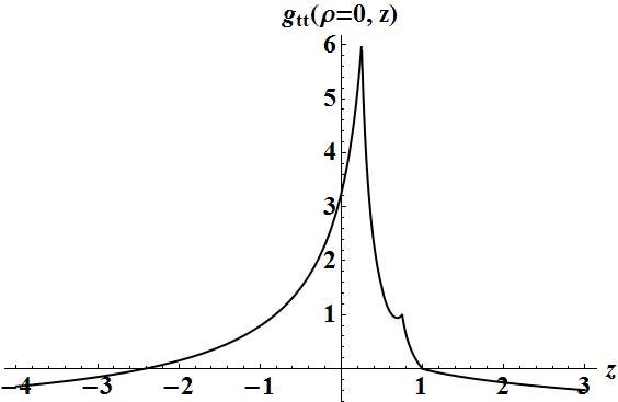
Figure 5.1: $g_{tt}|_{\rho=0}$ as a function of $z$ for $a_{1}=0$, $a_{2}=1$, $a_{3}=3/4$, $a_{4}=1/2$, $a_{5}=1/4$. In this case the ergosurface encloses both horizons.

5.4.4 $g_{\rho\rho}$ and $g_{zz}$

The metric functions $g_{\rho\rho}=g_{zz}$ on $\rho=0$, $z\in(a_{1},a_{5})$ equal

$$-\frac{a_{4}-z}{2(a_{3}-z)(z-a_{5})}\;,$$ (5.21)

and are therefore smooth there. By analyticity, the same expression is valid for $z\in(-\infty,a_{5})$.

The metric function $g_{\rho\rho}$ on $\rho=0$, $z\in(a_{5},a_{4})$ can be written as a rational function of $z$, with denominator

$${4(a_{1}-a_{2})^{2}(a_{2}-a_{4})(a_{2}-z)(a_{3}-a_{4})^{2}(a_{4}-z)(z-a_{5})}\;,$$

and is thus smooth near $\{\rho=0,z\in(a_{5},a_{4})\}$. One checks that for $z>a_{5}$ and close to $a_{5}$ we have

$$g_{\rho\rho}|_{\rho=0}=\frac{a_{4}-a_{5}}{2(a_{3}-a_{5})(z-a_{5})}+O(1)\;,$$ (5.22)

leading to a pole of order one when $a_{5}$ is approached from above. Comparing with (5.21) one finds that $|z-a_{5}|\times g_{\rho\rho}|_{\rho=0}$ is continuous at $a_{5}$.

Next, for $z<a_{4}$ and close to $a_{4}$ we have

$$g_{\rho\rho}|_{\rho=0}=\frac{a_{5}-a_{4}}{2(a_{3}-a_{4})(z-a_{4})}+O(1)\;,$$ (5.23)

leading to a pole of order one when $a_{4}$ is approached from below.

The metric function $g_{\rho\rho}$ on $\rho=0$, $z\in(a_{4},a_{3})$ equals

$$-\frac{z-a_{5}}{2(z-a_{3})(z-a_{4})}$$ (5.24)

with simple poles at $a_{4}$ and $a_{3}$. Comparing with (5.23) one finds that

$$|z-a_{4}|\times g_{\rho\rho}|_{\rho=0}$$

is continuous at $a_{4}$.

The metric function $g_{\rho\rho}$ on $\rho=0$, $z\in(a_{3},a_{2})$ can be written as a rational function of $z$, with denominator

$$4(a_{1}-a_{2})^{2}(a_{1}-a_{3})(a_{2}-a_{3})(a_{3}-a_{4})^{2}(a_{1}-z)(a_{2}-z)(a_{3}-z)(z-a_{5})\;,$$

which has been obtained by substituting in $k$, but neither $c_{1}$ nor $c_{2}$. For $z>a_{3}$ and close to $a_{3}$ we have

$$g_{\rho\rho}|_{\rho=0}=\frac{a_{3}-a_{5}}{2(a_{3}-a_{4})(z-a_{3})}+O(1)\;,$$ (5.25)

and there is a first order pole when $z=a_{3}$ is approached from above. Comparing with (5.24) one finds that $|z-a_{3}|\times g_{\rho\rho}|_{\rho=0}$ is continuous at $a_{3}$.

Again, for $z<a_{2}$ and close to $a_{2}$ we have

$$g_{\rho\rho}|_{\rho=0}=\frac{(a_{1}-a_{3})(a_{3}-a_{5})\big{(}2(a_{2}-a_{3})(a_{2}-a_{4})+(a_{2}-a_{5})c_{2}^{2}\big{)}}{4(a_{1}-a_{2})(a_{2}-a_{3})(a_{3}-a_{4})^{2}(a_{2}-z)}+O(1)\;,$$ (5.26)

Since $c_{2}$ is real, the numerator of the leading term does not vanish. Therefore, $g_{\rho\rho}|_{\rho=0}$ has a first order pole when $z=a_{2}$ is approached from below.

The metric function $g_{\rho\rho}$ on $\rho=0$, $z\in(a_{2},\infty)$ can be written as a rational function of $z$, with denominator${}^{\mbox{\scriptsize\ref{fnnoc_2sub}}}$

$$4(a_{1}-a_{2})^{2}(a_{3}-a_{4})^{2}(-a_{2}+a_{4})(a_{2}-z)(a_{3}-z)(-a_{5}+z)\;.$$

Finally, for $z>a_{2}$ and close to $a_{2}$ we have

$$g_{\rho\rho}|_{\rho=0}=-\frac{(a_{1}-a_{3})(a_{3}-a_{5})(2(a_{2}-a_{3})(a_{2}-a_{4})+(a_{2}-a_{5})c_{2}^{2})}{4(a_{1}-a_{2})(a_{2}-a_{3})(a_{3}-a_{4})^{2}(a_{2}-z)}+O(1)\;.$$ (5.27)

This coincides with (5.26) except for an overall sign. Again, with $c_{2}$ being real the numerator of the leading term cannot vanish, so the limits from above and from below of $|z-a_{2}|\times g_{\rho\rho}|_{\rho=0}$ at $z=a_{2}$ are different from zero, and coincide.

5.4.5 $g_{t\psi}$ and $g_{\psi\psi}$

We pass now to the singularities of

$$g_{t\psi}=-\frac{H_{y}}{H_{x}}\left(\frac{\omega_{\psi}}{H_{y}}+q\right)$$

on the axis $\rho=0$. It turns out that the calculations here are very similar to those for $g_{tt}$, keeping in mind that the interval $(-\infty,a_{5})$ was handled in Section 2. In particular the lack of zeros of the relevant denominators on each subinterval of the $z$–axis is established in exactly the same way as for $g_{tt}$, while continuity at the $a_{i}$’s is obtained by checking the left and right limits. This results most likely from the rewriting

$$g_{t\psi}=-\frac{F\omega_{\psi}+qFH_{y}}{FH_{x}}\;,$$

and noting that, away from the $a_{i}$’s, any infinities of $g_{t\psi}|_{\rho=0}$ can only result from zeros of $FH_{x}$. In any case, a Mathematica calculation shows that no further infinities in $g_{t\psi}|_{\rho=0}$ arise on the axis from $F\omega_{\psi}+qFH_{y}$, and in fact the denominators of $g_{t\psi}|_{\rho=0}$, when this last function is written as a rational function of the $z$’s, $a_{i}$’s, and the $c_{i}$’s, coincide with those of $g_{tt}|_{\rho=0}$. So, we find that $g_{t\psi}$ is smooth near

$$I:=\{\rho=0,z\in(-\infty,a_{5})\cup(a_{5},a_{4})\cup(a_{4},a_{3})\cup(a_{3},a_{2})\cup(a_{2},+\infty)\}\;.$$ (5.28)

For the remaining points $a_{2},\ldots,a_{5}$, we write instead

$$g_{t\psi}=g_{tt}\left(\frac{\omega_{\psi}}{H_{y}}+q\right)\;.$$ (5.29)

Using Mathematica we verified that the left and right limits of $(\omega_{\psi}/H_{y})|_{\rho=0}$ at $a_{i=1,5,4,3}$ are equal, but the left and right limit at $a_{2}$ is not. These are, respectively:

$\frac{2(a_{2}-a_{4})}{c_{2}}$ for $a_{1}$,

$\frac{2(a_{1}-a_{2})(a_{1}-a_{4})(a_{2}-a_{4})}{(a_{2}-a_{4})(a_{1}-a_{5})c_{1}+(a_{4}-a_{1})(a_{2}-a_{5})c_{2}}$ for $a_{5}$, $a_{4}$,

$\frac{2(a_{1}-a_{2})(a_{1}-a_{3})(a_{2}-a_{3})}{(a_{2}-a_{3})(a_{1}-a_{5})c_{1}+(a_{3}-a_{1})(a_{2}-a_{5})c_{2}}$ for $a_{3}$, $a_{2}^{-}$,

$\frac{2(a_{1}-a_{2})(a_{1}-a_{3})c_{2}}{2(a_{1}-a_{3})(a_{2}-a_{4})+(a_{1}-a_{5})c_{1}c_{2}}$ for $a_{2}^{+}$.

(Note that the first line above contains an inverse power of $c_{2}$, and so the case $c_{2}=0$ requires separate attention; this is handled in Section 5.8.1). On the other hand, the numerator of $g_{tt}$ on $\rho=0$ has already been analysed in Section 5.4.3, we repeat the formulae for the convenience of the reader

$\sim c_{2}^{2}$ for $a_{1}$ (see (2.2)),

$\sim((a_{2}-a_{4})(a_{1}-a_{5})c_{1}+(a_{4}-a_{1})(a_{2}-a_{5})c_{2})^{2}$ for $a_{5}$, $a_{4}$,

$\sim((a_{2}-a_{3})(a_{1}-a_{5})c_{1}+(a_{3}-a_{1})(a_{2}-a_{5})c_{2})^{2}$ for $a_{3}$,

$\sim((a_{2}-a_{3})(a_{1}-a_{5})c_{1}+(a_{3}-a_{1})(a_{2}-a_{5})c_{2})^{2}(a_{2}-z)$ near $a_{2}^{-}$,

$\sim(2(a_{1}-a_{3})(a_{2}-a_{4})+(a_{1}-a_{5})c_{1}c_{2})^{2}(a_{2}-z)$ near $a_{2}^{+}$.

We note that the $z$-independent terms above all have the same sign when $c_{1}c_{2}>0$, hence they are not identically zero. Thus the factors displayed here in the numerator of $g_{tt}$ can be cancelled with the corresponding factors in the denominator in the product $g_{tt}\times(\omega_{\psi}/H_{y})$ arising in (5.29). This implies that $g_{t\psi}|_{\rho=0}$ is continuous for $z\in\mathbb{R}$.

Consider next $g_{\psi\psi}|_{\rho=0}$,

$$g_{\psi\psi}=g_{tt}\left(\frac{\omega_{\psi}}{H_{y}}+q\right)^{2}-\frac{G_{y}}{g_{tt}}\;.$$

A Mathematica calculation shows again that the denominator of this function, when written as a rational function of $z$ and the $a_{i}$’s, coincides with the denominator of $g_{tt}|_{\rho=0}$, which has already been shown to have no zeros. This, implies that $g_{\psi\psi}|_{\rho=0}$ is smooth near the set appearing in (5.28).

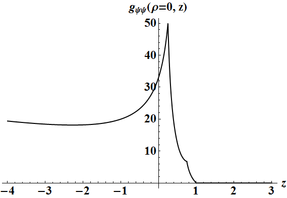
Figure 5.2: The graph of $g_{\psi\psi}$ on the axis for $a_{1}=0,a_{5}=\tfrac{1}{4},a_{4}=\tfrac{1}{2},a_{3}=\tfrac{3}{4},a_{2}=1.$

From what has been said so far, to prove continuity of $g_{\psi\psi}$ it remains to establish continuity of $G_{y}/g_{tt}$ at $z=a_{i}$. Now, $G_{y}$ is continuous on $\rho=0$ for $z\in\mathbb{R}$ and vanishes for $z\geq a_{3}$ (see Table 5.1) so $g_{\psi\psi}|_{\rho=0}$ is continuous at $\{a_{5},a_{4},a_{3},a_{2}\}$. We conclude that $g_{\psi\psi}$ is smooth near the set in (5.28), and that $g_{\psi\psi}|_{\rho=0}$ is continuous at all $z\in\mathbb{R}$.

However, the above is not the whole story about $g_{\psi\psi}$, as we need to know where $g_{\psi\psi}|_{\rho=0}$ vanishes; such points correspond either to lower dimensional orbits, or to closed null curves.

It already follows implicitly from Section 3 that $g_{\psi\psi}|_{\rho=0}=0$ for $z>a_{2}$ and, in fact, in that interval of $z$’s we have

$$g_{\psi\psi}=g_{\rho\rho}(1+O(\rho^{2}))\rho^{2}\;,$$ (5.30)

as needed for a regular “axis of rotation”. This formula is obtained by a direct Mathematica calculation, in the spirit of the ones already done in this section. We emphasize that we are not claiming uniformity of the error term $O(\rho^{2})$ above as $a_{2}$ is approached.

Note that $g_{\rho\rho}>0$ away from the axis, and it follows from (5.30) that $g_{\psi\psi}>0$ for $z>a_{2}$ and $\rho>0$ small enough.

The question of the sign of $g_{\psi\psi}|_{\rho=0}$ on the remaining axis intervals is addressed in Section 5.8.3 under the hypothesis that $c_{2}=0$. In Appendix B we give numerical evidence that $g_{\psi\psi}|_{\rho=0}$ is positive on $\{z<a_{2}\}$ for general $c_{2}$’s, see Figure B.2. The values of $g_{\psi\psi}|_{\rho=0}$ at $z=a_{i}$ for $i=5,4,3$ can be easily obtained by direct limits computation. As expected from the continuity established earlier the right and left limits coincide and are equal to

$\frac{(a_{5}-a_{3})(q(c_{1}(a_{1}-a_{5})(a_{2}-a_{4})+c_{2}(a_{4}-a_{1})(a_{2}-a_{5}))+2(a_{1}-a_{2})(a_{1}-a_{4})(a_{2}-a_{4}))^{2}}{(a_{1}-a_{5})(a_{5}-a_{2})(a_{5}-a_{4})(a_{2}c_{1}-a_{1}c_{2}+a_{4}(c_{2}-c_{1}))^{2}}$ for $a_{5}$,

$\frac{(q(c_{1}(a_{1}-a_{5})(a_{2}-a_{4})+c_{2}(a_{4}-a_{1})(a_{2}-a_{5}))+2(a_{1}-a_{2})(a_{1}-a_{4})(a_{2}-a_{4}))^{2}}{2(a_{1}-a_{2})^{2}(a_{1}-a_{4})(a_{4}-a_{2})(a_{4}-a_{5})}$ for $a_{4}$,

$\frac{(q(c_{1}(a_{1}-a_{5})(a_{2}-a_{3})+c_{2}(a_{3}-a_{1})(a_{2}-a_{5}))+2(a_{1}-a_{2})(a_{1}-a_{3})(a_{2}-a_{3}))^{2}}{2(a_{1}-a_{2})^{2}(a_{1}-a_{3})(a_{3}-a_{2})(a_{3}-a_{5})}$ for $a_{3}$.

From the ordering of $a_{i}$’s (A.15) it follows that $g_{\psi\psi}(\rho=0,z=a_{i})>0$ for $i=5,4,3$ if the parameters are distinct.

Finally, we need to check the signature of the metric. A Mathematica calculation shows that near $I$, as defined in (5.28), we can write

$$\det g_{\mu\nu}=(f+O(\rho^{2}))\rho^{2}\;,$$ (5.31)

where $f$ is an analytic function of $z$; for example,

$$f=\left\{\begin{array}[]{ll}\frac{z-a_{4}}{2(a_{3}-z)(z-a_{5})}\;,&\hbox{$z<a_{5}$\;;}\\ \frac{z-a_{5}}{2(a_{3}-z)(z-a_{4})}\;,&\hbox{$a_{4}<z<a_{3}$\;.}\end{array}\right.$$ (5.32)

(No uniformity near the end points is claimed for the error term in (5.31).) The explicit formulae for $f$ on the remaining intervals are too long to be usefully cited here. We simply note that we already know that the determinant of the metric is strictly negative for $\rho>0$, and thus $f\leq 0$ on the axis by continuity. However, $f$ could have zeros, which need to be excluded. Clearly there are no such zeros in the intervals listed in (5.32). Next, in the region $z>a_{2}$ one finds that $f=-h^{2}$, where $h$ is a quadratic function of $c_{2}$. The discriminant of $h$ with respect to $c_{2}$ reads

$$32(a_{1}-a_{2})^{2}(a_{1}-a_{3})^{4}(a_{2}-a_{4})^{2}(a_{1}-z)^{2}(a_{3}-z)(a_{4}-z)(a_{5}-z)\;.$$

This is strictly negative for $z>a_{2}$ and we conclude that $f$ does not vanish on this interval.

Taking into account the polar character of the coordinates $(\rho,\varphi)$ and $(\rho,\psi)$ near the relevant intervals of $z$, what has been said so far together with formula (5.31) implies that $g$ is a smooth Lorentzian metric on

$$\mathbb{R}^{4}\setminus\{\rho=0\;,\ z\in[a_{5},a_{4}]\cup[a_{3},a_{2}]\}\;.$$

The missing open intervals, and their end points, need separate attention; this will be addressed in Sections 5.5 and 5.6.

5.5 Extensions across Killing horizons

It is expected that the interval $z\in[a_{5},a_{4}]$ lying on the coordinate axis $\rho=0$, corresponds to a ring Killing horizon with topology $\mathbb{R}\times S^{1}\times S^{2}$, while $z\in[a_{3},a_{2}]$ corresponds to a spherical Killing horizon, with topology $\mathbb{R}\times S^{3}$. The aim of this section is to establish this, modulo possibly the end points where the axis meets the Killing horizon; this will be addressed in the next section. The construction mimics the corresponding extension procedure for the Kerr metric, see also [7, Section 3] or [1].

Let $a\in\mathbb{R}$ and let $m>0$ be given by

$$m^{2}=\left(\frac{a_{j}-a_{i}}{2}\right)^{2}+a^{2}\;,$$

set $r_{\pm}=m\pm\sqrt{m^{2}-a^{2}}$. As a first step of the construction of an extension on $[a_{i},a_{j}]=[a_{5},a_{4}]$ or $[a_{i},a_{j}]=[a_{3},a_{2}]$ we introduce the usual coordinates $\tilde{r}$ and $\tilde{\theta}$ for the Kerr metric:

$$\tilde{r}=\frac{R_{i}+R_{j}}{2}+m\;,\qquad\tilde{\theta}=\cos^{-1}\left(\frac{R_{j}-R_{i}}{a_{i}-a_{j}}\right)\;,$$ (5.33)

with inverse transformation (see, e.g., [9, (1.133), p. 27])

$$\rho = \sqrt{{\tilde{r}^{2}-2m\tilde{r}+a^{2}}}\,\sin(\tilde{\theta})\equiv\sqrt{{(\tilde{r}-r_{-})(\tilde{r}-r_{+})}}\,\sin(\tilde{\theta})\;,$$ (5.34)

$$z = \frac{a_{i}+a_{j}}{2}+{(\tilde{r}-m)}\,\cos(\tilde{\theta})\;.$$ (5.35)

Note that in the above conventions we have $a_{j}>a_{i}$.

In the $(\tilde{r},\tilde{\theta})$ coordinates the flat metric $\gamma:=d\rho^{2}+dz^{2}$ remains diagonal,

$$\gamma = \Big{(}(\tilde{r}-m)^{2}-\left(m^{2}-a^{2}\right)\cos^{2}(\tilde{\theta})\Big{)}$$ (5.36)

$$\phantom{xxxxx}\times\left(\frac{d\tilde{r}^{2}}{(\tilde{r}-m)^{2}-(m^{2}-a^{2})}+d\tilde{\theta}^{2}\right)$$

$$= {\left(\frac{\rho^{2}}{\sin^{2}\tilde{\theta}}+(m^{2}-a^{2})\sin^{2}\tilde{\theta}\right)}\left(\frac{\sin^{2}\tilde{\theta}}{\rho^{2}}d\tilde{r}^{2}+d\tilde{\theta}^{2}\right)$$ (5.37)

$$= {R_{i}R_{j}}\left(\frac{d\tilde{r}^{2}}{{(\tilde{r}-r_{-})(\tilde{r}-r_{+})}}+d\tilde{\theta}^{2}\right)$$ (5.38)

$$= {R_{i}R_{j}}\left(\frac{2\left(R_{i}R_{j}+(z-a_{i})(a_{j}-z)-\rho^{2}\right)}{\rho^{2}(a_{i}-a_{j})^{2}}d\tilde{r}^{2}+d\tilde{\theta}^{2}\right)\;,$$ (5.39)

where the various forms of the metric $\gamma$ have been listed for future reference.

The essential parameter above is $m^{2}-a^{2}$, in the sense that a change of $m$ and $a$ that keeps $m^{2}-a^{2}$ fixed can be compensated by a translation in $\tilde{r}$, without changing the explicit form of $\gamma$. The replacement of $\sqrt{m^{2}-a^{2}}$ by $-\sqrt{m^{2}-a^{2}}$ can be compensated by a change of the sign of $(\tilde{r}-m)$, which again does not change the explicit form of $\gamma$.

We have, near $\rho=0$, for $a_{i}<z<a_{j}$, with error terms not necessarily uniform over compact sets of $z$,

$$\gamma_{\tilde{r}\tilde{r}} = \frac{4(a_{i}-z)^{2}(a_{j}-z)^{2}}{\rho^{2}(a_{i}-a_{j})^{2}}+O(1)\;,$$ (5.40)

$$\gamma_{\tilde{\theta}\tilde{\theta}} = |(z-a_{i})(z-a_{j})|+O(\rho^{2})\;.$$ (5.41)

Now, the Black Saturn metric depends upon $\rho$ through $\rho^{2}$ only, with the latter being an analytic function of $\tilde{r}$ and $\tilde{\theta}$. In the new coordinate system all the metric functions extend analytically across $\{\rho=0,z\in(a_{i},a_{j})\}$ except $g_{\tilde{r}\tilde{r}}$, which has a first order pole in $\tilde{r}$ at $\tilde{r}=r_{\pm}$. In the original coordinate system we start with $\tilde{r}>r_{+}$ and it is not clear whether or not $r=r_{-}$ can be reached in the analytic extension, but we need to get rid of the pole at $\tilde{r}=r_{+}$ in any case. For this, it is convenient to continue with a general discussion. We consider a coordinate system $(x^{\mu},y)\equiv(x^{0},x^{i})\equiv(x^{0},x^{A},y)$, where $\mu$ runs from $0$ to $n-1$, and we suppose that:

1. The metric functions $g_{\mu\nu}$ are defined and real analytic near $y=y_{0}$, except for $g_{yy}$ which is meromorphic with a pole of order one at $y_{0}$.

2. The determinant of the metric is bounded away from zero near $y=y_{0}$.

3. There exists a Killing vector field $\xi$ of the form

   $$\xi=\partial_{0}+\alpha^{i}\partial_{i}\;,$$

   for some set of constants $\alpha^{i}$, such that all the functions

   $$g_{\mu\nu}\xi^{\mu}$$

   vanish at $y=y_{0}$.

In our case the first condition has just been verified with

$$y=\tilde{r}\;,\quad y_{0}=r_{\pm}\;.$$

The determinant condition holds by inspection of the metric, see Tables 5.1 and 5.2.

The third condition is verified by a Mathematica calculation, leading to a Killing vector $\partial_{t}+\Omega_{S^{3}}\partial_{\psi}$, where

$$\Omega_{S^{3}}=-\left(\frac{2(a_{1}-a_{2})(a_{1}-a_{3})(a_{2}-a_{3})}{(a_{2}-a_{3})(a_{1}-a_{5})c_{1}+(a_{3}-a_{1})(a_{2}-a_{5})c_{2}}+q\right)^{-1}\;,$$

satisfying the condition on $(a_{3},a_{2})$, and the Killing vector $\partial_{t}+\Omega_{S^{1}\times S^{2}}\partial_{\psi}\;,$ with

$$\Omega_{S^{1}\times S^{2}}=-\left(\frac{2(a_{1}-a_{2})(a_{1}-a_{4})(a_{2}-a_{4})}{(a_{2}-a_{4})(a_{1}-a_{5})c_{1}+(a_{4}-a_{1})(a_{2}-a_{5})c_{2}}+q\right)^{-1}\;,$$

satisfying the condition on $(a_{5},a_{4})$. A rather lengthy Mathematica calculation shows that the $\Omega$’s are finite for distinct $a_{i}$’s.

We introduce new coordinates $(\hat{x}^{\mu},\hat{y})\equiv(\hat{x}^{0},\hat{x}^{A},\hat{y})\equiv(\hat{x}^{0},\hat{x}^{i})$ by the formula

$$\hat{x}^{0}=x^{0}\;,\quad\hat{x}^{i}=x^{i}-\alpha^{i}x^{0}\;.$$ (5.42)

This coordinate transformation has Jacobian one. Writing $g_{\hat{\mu}\hat{\nu}}$ for $g(\partial_{\hat{x}^{\mu}},\partial_{\hat{x}^{\mu}})$, our hypotheses imply that we can write

$$g_{\hat{0}\hat{\mu}}=(y-y_{0})\chi_{\hat{\mu}}\;,\qquad g_{\hat{y}\hat{y}}=\frac{h}{(y-y_{0})}\;,$$ (5.43)

for some functions $\chi_{\hat{\mu}}$, $h$, all analytic near $y_{0}$.

Since the metric functions are now independent of $\hat{x}^{0}$, the next coordinate transformation

$$d\tilde{x}^{0}=d\hat{x}^{0}+f(\hat{y})d\hat{y}\;,\quad\tilde{x}^{A}=\hat{x}^{A}\;,\quad\tilde{y}=\hat{y}\;,$$

again with Jacobian one, does not affect the analyticity properties of the functions involved. We have

$$g_{\hat{0}\hat{0}}(d\hat{x}^{0})^{2}+g_{\hat{y}\hat{y}}d\hat{y}^{2} = (y-y_{0})\chi_{\hat{0}}\big{(}d\tilde{x}^{0}-fd\hat{y}\big{)}^{2}+\frac{h}{(y-y_{0})}d\hat{y}^{2}$$ (5.44)

$$= (y-y_{0})\chi_{\hat{0}}(d\tilde{x}^{0})^{2}-2(y-y_{0})\chi_{\hat{0}}fd\tilde{x}^{0}d\hat{y}$$

$$+\frac{h+(y-y_{0})^{2}\chi_{\hat{0}}f^{2}}{(y-y_{0})}d\hat{y}^{2}\;.$$

Assume that

$$\kappa:=-\lim_{y\to y_{0}}\frac{h}{\chi_{\hat{0}}}$$

is a positive constant. Keeping in mind that $\chi_{\hat{0}}$ is negative while $h$ is positive, and choosing $f$ as

$$f=\frac{\sqrt{\kappa}}{y-y_{0}}\;,$$ (5.45)

one obtains a smooth analytic extension of the metric through $y=y_{0}$, since then the singularity in (5.44) is removable; similarly

$$g_{\hat{0}\hat{i}}d\hat{x}^{0}d\hat{x}^{i} = (y-y_{0})\chi_{\hat{i}}\big{(}d\tilde{x}^{0}-fd\hat{y}\big{)}d\hat{x}^{i}$$

$$= (y-y_{0})\chi_{\hat{i}}d\tilde{x}^{0}d\hat{x}^{i}-\chi_{\hat{i}}\sqrt{\kappa}d\hat{y}d\hat{x}^{i}\;.$$

The determinant of the metric in the coordinate system $\tilde{x}^{\mu}$ equals that in the original coordinates, and so the extended metric is Lorentzian near $y=y_{0}$.

It remains to show that this procedure applies to the BS metric, with

$$x^{0}=t\;,\ y-y_{0}:=\tilde{r}-r_{+}\;,\ (x^{A})=(\varphi,\psi,\tilde{\theta})\ \;,$$

where $\tilde{r}$ and $\tilde{\theta}$ have been defined in (5.33). We have

$$\tilde{r}-r_{+}=\frac{(a_{j}-a_{i})\rho^{2}}{4(a_{j}-z)(z-a_{i})}+O(\rho^{4})\;,$$

hence

$$(\tilde{r}-r_{-})\sin^{2}\tilde{\theta}=\frac{4(a_{j}-z)(z-a_{i})}{(a_{j}-a_{i})}+O(\rho^{2})\;,$$

with the error term not uniform in $z$ near the end points. On $(a_{5},a_{4})$ or on $(a_{3},a_{2})$ one needs to calculate the limits

$$h|_{\tilde{r}=r_{+}} = \lim_{\rho\to 0}\frac{H_{x}k^{2}P}{(\tilde{r}-r_{-})\sin^{2}\tilde{\theta}}\times\lim_{\rho\to 0}(\rho^{2}\gamma_{\tilde{r}\tilde{r}})\;.$$

Letting $\Omega=\Omega_{S^{1}\times S^{2}}$ on $(a_{5},a_{4})$, respectively $\Omega=\Omega_{S^{3}}$ on $(a_{3},a_{2})$, one further needs

$$\chi_{\hat{0}}|_{\tilde{r}=r_{+}} = \lim_{\rho\to 0}\big{(}\rho^{-2}g(\partial_{t}+\Omega\partial_{\psi},\partial_{t}+\Omega\partial_{\psi})(\tilde{r}-r_{-})\sin^{2}\tilde{\theta}\big{)}\;.$$

A surprisingly involved Mathematica calculation shows that at $\rho=0$ the quotient ${h}/{\chi_{0}}$ equals, up to sign,

$$\frac{(a_{4}-a_{5})(2(a_{1}-a_{2})(a_{1}-a_{4})(a_{2}-a_{4})+((a_{2}-a_{4})(a_{1}-a_{5})c_{1}+(a_{4}-a_{1})(a_{2}-a_{5})c_{2})q)^{2}}{8(a_{1}-a_{2})^{2}(a_{2}-a_{4})(a_{3}-a_{4})^{2}(a_{4}-a_{1})}$$

on $(a_{5},a_{4})$, and

$$\frac{(a_{3}-a_{5})(2(a_{1}-a_{2})(a_{1}-a_{3})(a_{2}-a_{3})+((a_{2}-a_{3})(a_{1}-a_{5})c_{1}+(a_{3}-a_{1})(a_{2}-a_{5})c_{2})q)^{2}}{8(a_{1}-a_{2})^{2}(a_{2}-a_{3})(a_{3}-a_{1})(a_{3}-a_{4})^{2}}$$

on $(a_{3},a_{2})$. As those limits are constants, we have verified that, within the current range of parameters, the Black Saturn metric can be extended across two non-degenerate Killing horizons.

5.6 Intersections of axes of rotations and horizons

It follows from (5.33) that

$$R_{i} = \tilde{r}-r_{+}+\frac{a_{j}-a_{i}}{2}(\cos\tilde{\theta}+1)\;,$$ (5.46)

$$R_{j} = \tilde{r}-r_{+}+\frac{a_{j}-a_{i}}{2}(1-\cos\tilde{\theta})\;,$$ (5.47)

$$\mu_{i} = (\tilde{r}-r_{+})(1-\cos\tilde{\theta})\;,$$ (5.48)

$$\mu_{j} = (\tilde{r}-r_{-})(1-\cos\tilde{\theta})\;,$$ (5.49)

so that $\mu_{i}$, $\mu_{j}$, $R_{i}$ and $R_{j}$ are smooth functions of $\tilde{r}$ and $\cos\tilde{\theta}$. Furthermore, it follows from (5.34) that the function $\rho^{2}$ is a smooth function of $\tilde{r}$ and of $\sin^{2}\tilde{\theta}=1-\cos^{2}\tilde{\theta}$, similarly $z$ is smooth in $\cos\tilde{\theta}$ by (5.35), which implies that the remaining $\mu_{\ell}$’s (compare (5.51)-(5.52)) are smooth in $\tilde{r}$ and $\cos\tilde{\theta}$.

Now, consider any rational function, say $W$, of the $\mu_{i}$’s and $\rho^{2}$, which is bounded near $\tilde{r}=r_{+}$, $\tilde{\theta}=0$. Boundedness implies that any overall factors of $\tilde{r}-r_{+}$ in the denominator of $W$ are cancelled out by a corresponding overall factor in the numerator, leaving behind a denominator $d(\tilde{r},\tilde{\theta})$ which can be written in the form

$$d(\tilde{r},\tilde{\theta})=\mathring{f}(\cos\tilde{\theta})+(\tilde{r}-r_{+})\mathring{g}(\tilde{r},\cos\tilde{\theta})\;,$$

for some functions $\mathring{f}$ and $\mathring{g}$ which are smooth in their respective arguments. If

$$d(\tilde{r}=r_{+},0)\equiv\mathring{f}(1)$$

does not vanish at $\tilde{\theta}=0$, then the denominator $d$ is bounded away from zero near $\tilde{r}=r_{+}$ and $\tilde{\theta}=0$. This in turn implies that $1/d$ is smooth in a neighbourhood of the point concerned, and therefore so is $W$.

An identical argument applies at $\tilde{\theta}=\pi$.

This reasoning does not seem to apply to $\omega_{\psi}$, because of the square roots there. However, as mentioned in Appendix A.1, these appear in the form

$$\sqrt{\frac{M_{0}M_{1}}{G_{x}}}\;,\quad\sqrt{\frac{M_{0}M_{2}}{G_{x}}}\;,\quad\sqrt{\frac{M_{1}M_{4}}{G_{x}}}\;,\quad\sqrt{\frac{M_{2}M_{4}}{G_{x}}}\;.$$

One checks that the expressions under the square root are squares of rational functions of the $\mu_{i}$’s, and of $\rho^{2}$, and so the metric functions involving $\omega_{\psi}$ are also rational functions of the $\mu_{i}$’s and $\rho^{2}$.

Since we have already shown that the suitably reduced denominators of all the scalar products $g(X,Y)$, where $X,Y\in\{\partial_{t},\partial_{\psi},\partial_{\varphi}\}$, have no zeros at the axis points $\rho=0$, $z=a_{i}$, we conclude that the corresponding metric coefficients are analytically extendible, by allowing $\tilde{r}$ to become smaller than $r_{+}$, including near the intersections of axes of rotation with the Killing horizons.

One similarly establishes analytic extendibility of $g_{\tilde{t}\tilde{y}}$:

$$g_{\tilde{y}\tilde{t}} = -\frac{(g_{tt}+2g_{t\psi}\Omega+g_{\psi\psi}\Omega^{2})\sqrt{\kappa}}{\tilde{r}-r_{+}}\;.$$

Here we have already verified that $g_{tt}+2g_{t\psi}\Omega+g_{\psi\psi}\Omega^{2}$ is an analytic function of $\tilde{r}$ and $\cos\tilde{\theta}$, and extendibility of $g_{\tilde{y}\tilde{t}}$ readily follows from the fact that $\Omega$ has been chosen so that this function vanishes at $\tilde{r}=r_{+}$.

Finally, $g_{\tilde{y}\tilde{y}}$ is given by the formula

$$g_{\tilde{y}\tilde{y}} = \frac{\sqrt{\kappa}g_{\tilde{y}\tilde{t}}+(\tilde{r}-r_{+})g_{\tilde{r}\tilde{r}}}{\tilde{r}-r_{+}}\;.$$ (5.50)

To analyse this metric function, by a Mathematica calculation we verified that the reduced denominator of $(\tilde{r}-r_{+})g_{\tilde{r}\tilde{r}}$ does not vanish at $\tilde{r}=r_{+}$, and hence this function extends across $\tilde{r}=r_{+}$ as an analytic function of $\tilde{r}$ and $\cos\tilde{\theta}$. Keeping in mind that the same has already been established for $\sqrt{\kappa}g_{\tilde{t}\tilde{y}}$, we find that the numerator of (5.50) extends across $\tilde{r}=r_{+}$ as an analytic function of $\tilde{r}$ and $\cos\tilde{\theta}$. Analytic extendibility of $g_{\tilde{y}\tilde{y}}$ follows again from standard factorisation properties of such functions.

We next analyse $g_{\tilde{\theta}\tilde{\theta}}$ near $\rho=0$, $z=a_{4}$. Now,

$$g_{\tilde{\theta}\tilde{\theta}} = H_{x}k^{2}P\gamma_{\tilde{\theta}\tilde{\theta}}=g_{\rho\rho}R_{i}R_{j}\;,$$

and we need to understand the behaviour of the functions above near $\tilde{r}=r_{+}$, $\tilde{\theta}\in\{0,\pi\}$. For $\ell\neq 5$ we have

$$\mu_{\ell}\mu_{5}+\rho^{2} = \left((\tilde{r}-r_{-})\sin^{2}\theta+\mu_{\ell}(1-\cos\tilde{\theta})\right)(\tilde{r}-r_{+})\;,$$ (5.51)

and since

$$\mu_{1}=\frac{\rho^{2}}{R_{1}+z-a_{1}}\approx\frac{\rho^{2}}{2(a_{4}-a_{1})}$$ (5.52)

near $\rho=0$, $z=a_{4}$, for $\ell=2,3$ we can write

$$\mu_{\ell}\mu_{4}+\rho^{2} = \left(\tilde{r}-r_{+}+\frac{\mu_{\ell}}{1+\cos\tilde{\theta}}\right)(\tilde{r}-r_{-})\sin^{2}\tilde{\theta}\;,$$ (5.53)

$$\mu_{\ell}\mu_{5}+\rho^{2} = \left(\tilde{r}-r_{-}+\frac{\mu_{\ell}}{1+\cos\tilde{\theta}}\right)(\tilde{r}-r_{+})\sin^{2}\tilde{\theta}\;,$$ (5.54)

$$\mu_{4}\mu_{5}+\rho^{2} = \frac{2(\tilde{r}-r_{-})}{1+\cos\tilde{\theta}}(\tilde{r}-r_{+})\sin^{2}\tilde{\theta}\;,$$ (5.55)

$$\mu_{1}\mu_{\ell}+\rho^{2} \approx \left(\frac{a_{\ell}-a_{4}}{a_{4}-a_{1}}+1\right)\rho^{2}$$ (5.56)

$$= \frac{a_{\ell}-a_{1}}{a_{4}-a_{1}}(\tilde{r}-r_{-})(\tilde{r}-r_{+})\sin^{2}\tilde{\theta}\;.$$

Finally, for $\ell=1,4,5$,

$$\mu_{1}\mu_{\ell}+\rho^{2} \approx \rho^{2}=(\tilde{r}-r_{-})(\tilde{r}-r_{+})\sin^{2}\tilde{\theta}\;.$$ (5.57)

Encoding this behaviour into a Mathematica calculation, one finds that $g_{\tilde{\theta}\tilde{\theta}}$ is uniformly bounded in a neighbourhood of $r=r_{+}$, $\cos\tilde{\theta}\in\{\pm 1\}$, with non-vanishing value of the denominator as needed above. This establishes smoothness. Similarly $g_{\varphi\varphi}/\sin^{2}\tilde{\theta}$ is smooth near those points.

Now, away from, and near to, the event horizons, the map $(\rho,z)\mapsto(\tilde{r},\tilde{\theta})$ is a smooth coordinate transformation. From what has been already established, the two-dimensional metric

$$g_{\tilde{\theta}\tilde{\theta}}d\tilde{\theta}^{2}+g_{\varphi\varphi}d\varphi^{2}$$ (5.58)

is thus a smooth metric for $\tilde{r}>r_{+}$, $\tilde{r}$ close to $r_{+}$, in particular there is no conical singularity at the rotation axis for $\partial_{\varphi}$ in this region. But the arguments just given show that this metric extends smoothly across $\tilde{r}=r_{+}$, which finishes the proof of smoothness of the whole metric up-to-and-beyond the horizon near $\tilde{r}=r_{+}$, $\tilde{\theta}=0$.

A similar analysis applies near $a_{5}$, $a_{3}$ and $a_{2}$; in this last case, one considers the two-dimensional metric

$$g_{\tilde{\theta}\tilde{\theta}}d\tilde{\theta}^{2}+g_{\psi\psi}d\psi^{2}$$

instead of (5.58).

5.7 Event horizons

Consider the manifold, say ${\mycal M}$, obtained by adding to the region $\tilde{r}>r_{+}$ those points in the region $r_{-}<\tilde{r}$ for which the metric is smooth and Lorentzian. Then the region $r_{-}<\tilde{r}\leq r_{+}$ is contained in a black hole region in the extended space-time, which can be seen as follows: Note, first, that $g^{yy}$ vanishes at ${\mycal H}:=\{\tilde{r}=r_{+}\}=\{y=y_{0}\}$, which shows that ${\mycal H}$ is the union of two null hypersurfaces. On each connected component of ${\mycal H}$ the corresponding Killing vector $X=\partial_{t}+\Omega\partial_{\psi}$ is timelike future pointing for $y>y_{0}$ close to $y_{0}$, and so by continuity $X$ is future pointing on ${\mycal H}$. This implies that ${\mycal H}$ is locally achronal in the extended space-time: if a future directed timelike curves crosses ${\mycal H}$ through a point $p\in{\mycal H}$, it does so towards that side of $T_{p}{\mycal H}$ which contains the component of the set of causal vectors at $p$ containing $X$. Since ${\mycal H}$ is a (closed) separating hypersurface in ${\mycal M}$, this implies that any timelike curve can cross ${\mycal H}$ only once. From what has been said it follows that the region $r_{-}<\tilde{r}\leq r_{+}$ is contained in a black hole region of $({\mycal M},g)$.

In particular we have shown that the black hole region is not empty. A standard argument (compare [2, Section 4.1]) shows that ${\mycal H}$ coincides with the black hole event horizon in ${\mycal M}$. Note that this is true independently of stable causality of $({\mycal M},g)$, or of stable causality of the d.o.c. in $({\mycal M},g)$.

Some more work is required to add the bifurcation surface of the horizon, a general procedure how to do this is described in [11].

5.8 The analysis for $c_{2}=0$

We turn our attention now to the Black Saturn solutions with $c_{2}=0$, where the formulae simplify sufficiently to allow a proof of stable causality of the d.o.c.

First note that (4.2) implies that the condition $c_{2}=0$ leads to $c_{1}\neq 0$ as the only restriction on $c_{1}$. However, it implies a fine-tuning of the parameters $a_{i}$. One may easily check that the minus sign solution for $c_{2}$ cannot vanish if the ordering (A.15) of the $a_{i}$’s is assumed. However the plus sign solution may lead to the vanishing $c_{2}$ under certain additional conditions. Namely the resulting equation

$$\sqrt{({a_{3}}-{a_{1}})({a_{2}}-{a_{4}})({a_{2}}-{a_{5}})({a_{3}}-{a_{5}})}=({a_{2}}-{a_{1}})({a_{3}}-{a_{4}})\;,$$

quadratic in $a_{5}$, may always be solved for $a_{5}=a_{5}(a_{1},a_{2},a_{3},a_{4})\in\mathbb{R}$; the condition that $0<a_{5}<a_{4}$ is then equivalent to

$$a_{4}<(a_{2}^{2}+a_{1}a_{3}-2a_{2}a_{3})/(a_{1}-a_{3})\;.$$ (5.59)

This is more transparent in terms of the variables $\kappa_{i}\in[0,1]$ defined by (5.3), as then (5.59) becomes

$$\kappa_{1}>\frac{1}{2-\kappa_{2}}\;,$$ (5.60)

see Figure 5.3.

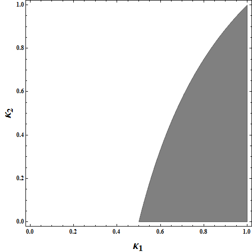
Figure 5.3: The variable $\kappa_{1}$ runs along the horizontal axis, while $\kappa_{2}$ runs along the vertical one. The inequality (5.60) corresponds to the shaded region.

In the further analysis one should keep in mind that $a_{5}$ is no more an independent parameter.

Notice that $c_{2}=0$ implies $q=0$ and $k=1$.

5.8.1 Smoothness at the axis

Smoothness of the Black Saturn solution for $\rho>0$, proved in Section 5.3, holds also for the $c_{2}=0$ case, hence only the analysis on the axis of rotation needs separate attention. We shall proceed in the same way as in Section 5.4.

We start with an analysis of the behaviour of $g_{\psi\psi}$ on the axis. For $z<a_{1}$ it may be written as a rational function

$$-\frac{2({a_{1}}-{a_{3}})^{2}({a_{2}}-z)(z-{a_{2}})(z-{a_{4}})(z-{a_{5}})+{c_{1}}^{2}({a_{1}}-{a_{2}})^{2}({a_{1}}-{a_{5}})^{2}({a_{3}}-z)}{({a_{1}}-{a_{3}})^{2}({a_{1}}-z)(z-{a_{2}})(z-{a_{4}})}\;.$$

To avoid the singularity at $z=a_{1}$ we need to fix $c_{1}$ as to have a finite limit. Miraculously, this condition leads to the same formula $c_{1}$ as obtained in section 2 for $c_{2}\neq 0$. This is somewhat unexpected, since we have set $c_{2}$ to zero as an alternative to fixing $c_{1}$. With this choice of $c_{1}$ regularity on the axis of many metric functions has already been established, and we would be done if not for the fact that some of the formulae derived so far involve explicit inverse powers of $c_{2}$. So it is necessary to repeat the analysis at the axis from scratch.

Several formulae are much simpler now. For instance, one checks that in the region $a_{1}<z\leq a_{5}$ on the axis $g_{\psi\psi}$ is given by the same formula as for $z<a_{1}$. Hence we conclude, that $g_{\psi\psi}$ is smooth and bounded for $\{\rho=0,\,z<a_{5}\}$.

In the subsequent axis interval, $a_{5}<z<a_{4}$, $g_{\psi\psi}$ is a rational function with denominator

$$2({a_{1}}-{a_{2}})^{2}({a_{1}}-{a_{4}})^{2}({a_{3}}-z)({a_{5}}-z)-{c_{1}}^{2}({a_{1}}-{a_{5}})^{2}({a_{2}}-z)^{2}({a_{4}}-z)\;,$$

which cannot vanish, being a sum of two negative terms. At both end points of the investigated interval one of the terms in non-zero, which shows boundedness.

Moving further to the right we obtain a simple formula for $g_{\psi\psi}$:

$$\frac{2(a_{1}-z)(a_{2}-z)}{(a_{5}-z)}\;,$$ (5.61)

which immediately implies continuity for $a_{4}\leq z\leq a_{3}$. We note that this is strictly positive, and therefore near that axis interval $g_{\psi\psi}$ is strictly positive as well.

In the region $a_{3}<z<a_{2}$ the denominator of $g_{\psi\psi}$ is more complicated:

$$(a_{1}-a_{5})^{2}c_{1}^{2}(a_{2}-z)^{2}(a_{3}-z)-2(a_{1}-a_{2})^{2}(a_{1}-a_{3})^{2}(a_{4}-z)(a_{5}-z),$$

but does not vanish, being a strictly negative sum of two non-positive terms.

In the region $z>a_{2}$ for vanishing $c_{2}$ the function $g_{\psi\psi}$ is proportional to $q^{2}$. Since $c_{2}=0$ implies $q=0$, we conclude that $g_{\psi\psi}$ vanishes for $z>a_{2}$, as already seen for general values of $c_{2}$ in any case.

The analysis of $g_{tt}$ is similar. For $\rho=0$ and $z<a_{5}$ the metric function $g_{tt}$ is a simple rational function,

$$\frac{(a_{1}-z)(z-a_{3})}{(z-a_{2})(z-a_{4})}\;,$$ (5.62)

which is clearly continuous in the region $z\leq a_{5}$. For $a_{5}<z<a_{4}$ the denominator of $g_{tt}$ reads

$$(a_{1}-a_{5})^{2}c_{1}^{2}(a_{2}-z)^{2}(a_{4}-z)+2(a_{1}-a_{2})^{2}(a_{1}-a_{4})^{2}(a_{3}-z)(z-a_{5})\;.$$ (5.63)

with both terms manifestly positive in the region $a_{5}\leq z\leq a_{4}$. We conclude that $g_{tt}$ is smooth on $a_{5}<z<a_{4}$, bounded on $a_{5}\leq z\leq a_{4}$.

Next, for $a_{4}<z<a_{3}$ the denominator of $g_{tt}$ reads

$$2(a_{1}-a_{2})^{2}(a_{1}-z)(z-a_{2})(z-a_{5})\;,$$

thus it cannot vanish for $a_{4}\leq z\leq a_{3}$. Moving further to the right we find the denominator of $g_{tt}$

$$(a_{1}-a_{5})^{2}c_{1}^{2}(a_{2}-z)^{2}(a_{3}-z)+2(a_{1}-a_{2})^{2}(a_{1}-a_{3})^{2}(a_{4}-z)(z-a_{5})$$

as a sum of manifestly negative terms on $a_{3}<z<a_{2}$. Also the end points are singularity-free. Finally, for $z>a_{2}$ $g_{tt}$ equals

$$\frac{(z-a_{2})(z-a_{4})}{(a_{1}-z)(z-a_{3})}\;,$$ (5.64)

hence it is continuous. This proves directly absence of singularities for $g_{tt}$ on the axis in the case of vanishing $c_{2}$.

The analysis of $g_{t\psi}$ can be carried out along the same lines, and is omitted.

5.8.2 Causality away from the axis

We have not been able to establish non-existence of closed timelike curves for a general Black Saturn solution, though we failed to find any in a numerical search, see Appendix B. However, if one imposes the condition $c_{2}=0$ the metric formulas simplify sufficiently to allow a direct analysis. Indeed, the explicit formula for $g_{\psi\psi}$ in the case of vanishing $c_{2}$ (and consequently $q=0$) reads

$$\frac{{\mu_{1}}{\mu_{2}}{\mu_{5}}\left(\rho^{2}\left({c_{1}}^{2}M_{1}+M_{0}\right)^{2}-4{c_{1}}^{2}M_{0}M_{1}{R_{1}}^{2}\right)}{\rho^{2}\left({c_{1}}^{2}M_{1}+M_{0}\right)\left(M_{0}{\mu_{1}}^{2}-{c_{1}}^{2}M_{1}\rho^{2}\right)}=:\frac{f(c_{1}^{2})}{g(c_{1}^{2})}\;.$$

Outside the axis ($\rho>0$) the ordering of $\mu_{i}$’s is the same as those of $a_{i}$’s and all the functions $M_{i}$ are strictly positive. Both the numerator and denominator of $g_{\psi\psi}$ can be regarded as quadratic functions of $c_{1}^{2}$. Let us first investigate the possible zeros of the denominator:

$$g(c_{1}^{2})=0\Rightarrow c_{1}^{2}=-\frac{M_{0}}{M_{1}}\text{ or }c_{1}^{2}=\frac{M_{0}\mu_{1}^{2}}{M_{1}\rho^{2}}\;.$$

Clearly only the second one is relevant since the first one would lead to an imaginary coefficient $c_{1}$. On the other hand, the equation $f(c_{1}^{2})=0$ has two solutions:

$$c_{\pm}^{2}=\frac{{M_{0}}\left(2{R_{1}}\left({R_{1}}\pm\sqrt{{R_{1}}^{2}-\rho^{2}}\right)-\rho^{2}\right)}{{M_{1}}\rho^{2}}\;.$$

To make this result more transparent let us express $R_{1}$ in terms of $\mu_{1}$ and $\rho$

$$R_{1}=\frac{\mu_{1}^{2}+\rho^{2}}{2\mu_{1}}\;.$$

Then $c_{\pm}^{2}$ may be written as

$$c_{\pm}^{2}=\frac{M_{0}}{{M_{1}}\rho^{2}}\,\frac{(\mu_{1}^{2}+\rho^{2})\left(\mu_{1}^{2}+\rho^{2}\pm|\mu_{1}^{2}-\rho^{2}|\right)-2\mu_{1}^{2}\rho^{2}}{2\mu_{1}^{2}}\;.$$

From the explicit form of $\mu_{1}$ one can easily see that $\text{sign}(\mu_{1}^{2}-\rho^{2})=\text{sign}(a_{1}-z)$, thus we have:

$$\text{for }z\leq a_{1} \displaystyle c_{-}^{2}=\frac{M_{0}\mu_{1}^{2}}{{M_{1}}\rho^{2}}\;, c_{+}^{2}=\frac{M_{0}\rho^{2}}{{M_{1}}\mu_{1}^{2}}\;,$$

$$\text{for }z\geq a_{1} \displaystyle c_{-}^{2}=\frac{M_{0}\rho^{2}}{{M_{1}}\mu_{1}^{2}}\;, c_{+}^{2}=\frac{M_{0}\mu_{1}^{2}}{{M_{1}}\rho^{2}}\;.$$

We see that in both regions one of the zeros $c_{\pm}^{2}$ of the numerator cancels the zero of the denominator, which provides an alternative explicit proof of regularity of $g_{\psi\psi}$ for $\rho>0$. Moreover we find:

$$g_{\psi\psi} = \frac{{\mu_{1}}{\mu_{2}}{\mu_{5}}M_{1}}{\rho^{2}\left({c_{1}}^{2}M_{1}+M_{0}\right)}\left(\frac{M_{0}\rho^{2}}{{M_{1}}\mu_{1}^{2}}-c_{1}^{2}\right)=\frac{{\mu_{2}}{\mu_{5}}\left({M_{0}\rho^{2}}-c_{1}^{2}{M_{1}}\mu_{1}^{2}\right)}{\rho^{2}{\mu_{1}}\left({c_{1}}^{2}M_{1}+M_{0}\right)}\;.$$

Keeping in mind that the parameter $c_{1}$ has been fixed to guarantee the regularity on the axis, to obtain a sign for $g_{\psi\psi}$ for $\rho>0$ it remains to show that the equality

$$c_{1}^{2}=\frac{M_{0}\rho^{2}}{{M_{1}}\mu_{1}^{2}}$$

can never be satisfied away from the axis. For this, we shall make use of the formula (5.8) expressing $c_{1}^{2}$ in terms of $\mu_{i}$’s. By subtracting the two formulae for $c_{1}^{2}$ we obtain

$$-\frac{{\mu_{5}}({\mu_{3}}-{\mu_{1}})\left({\mu_{1}}{\mu_{4}}+\rho^{2}\right)}{{\mu_{1}}^{4}{\mu_{3}}{\mu_{4}}({\mu_{1}}-{\mu_{2}})^{2}({\mu_{1}}-{\mu_{5}})^{2}\left({\mu_{1}}{\mu_{5}}+\rho^{2}\right)}\;\times\phantom{xxxxxxxxxxxxxx}$$

$$\Big{(}{\mu_{1}}^{3}({\mu_{1}}-{\mu_{2}})^{2}({\mu_{1}}-{\mu_{4}})({\mu_{1}}-{\mu_{5}})\left({\mu_{1}}{\mu_{3}}+\rho^{2}\right)\phantom{xxxxxxxxxxx}$$

$$+({\mu_{1}}-{\mu_{3}})\left({\mu_{1}}{\mu_{2}}+\rho^{2}\right)^{2}\left({\mu_{1}}{\mu_{4}}+\rho^{2}\right)\left({\mu_{1}}{\mu_{5}}+\rho^{2}\right)\Big{)}=0\;.$$

The overall multiplicative coefficient in the first line is strictly negative, whereas the term in parenthesis across the second and third lines is a polynomial in $\rho$ with coefficients that can be written in the following, manifestly negative form

$$\mu_{1}^{5}\left((\mu_{1}-\mu_{2})^{2}\mu_{3}(\mu_{1}-\mu_{4})+\mu_{5}\left(\mu_{2}^{2}(\mu_{4}-\mu_{3})+(\mu_{1}-\mu_{4})\mu_{3}(\mu_{2}+(\mu_{2}-\mu_{1}))\right)\right)$$

$$+\rho^{2}\mu_{1}^{3}\Big{(}\mu_{2}(\mu_{1}-\mu_{3})(2\mu_{4}\mu_{5}+\mu_{2}(\mu_{5}+\mu_{1}))$$

$$\phantom{\rho^{2}\mu_{1}^{3}\Big{(}}+(\mu_{4}-\mu_{1})\left(\mu_{2}^{2}(\mu_{5}-\mu_{3})+\mu_{1}((\mu_{1}-\mu_{2})-\mu_{2})(\mu_{5}-\mu_{1})\right)\Big{)}$$

$$+\rho^{4}\mu_{1}^{2}(\mu_{1}-\mu_{3})\left(\mu_{2}^{2}+\mu_{4}\mu_{5}+2\mu_{2}(\mu_{4}+\mu_{5})\right)$$

$$+\rho^{6}\mu_{1}(\mu_{1}-\mu_{3})(2\mu_{2}+\mu_{4}+\mu_{5})$$

$$+\rho^{8}(\mu_{1}-\mu_{3})\;.$$

It follows that $g_{\psi\psi}>0$ for $\rho>0$ when $c_{2}=0$.

It turns out that an alternative simpler argument for positivity can be given as follows: Using (5.8) we may write $g_{\psi\psi}$ in terms of $\mu_{i}$ and $\rho$. The functions $\mu_{i}$ satisfy the same ordering as $a_{i}$ (A.15) (see (5.2)). The strict version of the ordering (A.15) implies a strict ordering of the $\mu_{i}$’s for $\rho>0$. Assuming that, we may make the positivity of $g_{\psi\psi}$ explicit by expressing it in terms of the positive functions

$$\Delta_{51}=\mu_{5}-\mu_{1} \Delta_{45}=\mu_{4}-\mu_{5} \Delta_{34}=\mu_{3}-\mu_{4} \Delta_{23}=\mu_{2}-\mu_{3}$$, , , and . (5.65)

The numerator and denominator of $g_{\psi\psi}$ are polynomials in $\Delta_{ij}$, $\mu_{1}$ and $\rho$, the explicit form of which is too long to be usefully exhibited here. By inspection one finds that all coefficient of these polynomials are positive, and since the $\Delta_{ij}$’s, $\mu_{1}$ and $\rho$ are positive, both the numerator and denominator of $g_{\psi\psi}$ are positive.

5.8.3 Causality on the axis

We turn now our attention to the axis. By continuity, we know that $g_{\psi\psi}$ at $\rho=0$ is non-negative. It therefore suffices to exclude zeros of $g_{\psi\psi}|_{\rho=0}$. Equivalently, whenever we find a manifestly non-zero value of $g_{\psi\psi}(0,z)$, we know that this value cannot be negative.

Now, at $\rho=0$ and for $z<a_{1}$ we replace $z$ by $w:=z-a_{1}<0$, and find that $g_{\psi\psi}$ there is a rational function with denominator

$$(a_{1}-a_{3})(a_{1}-a_{2}+w)(a_{1}-a_{4}+w)\;,$$

which is seen to be strictly negative for $w\leq 0$. On the other hand, the numerator is a third-order polynomial in $w$:

$$2(a_{2}-a_{1})\times\Big{(}3a_{1}^{3}-a_{1}^{2}(a_{2}+2(2a_{3}+a_{4}+a_{5}))$$

$$\phantom{xxx}+a_{1}(2a_{2}a_{3}+3a_{3}(a_{4}+a_{5})+a_{4}a_{5})-a_{2}(a_{3}(a_{4}+a_{5})-a_{4}a_{5})-2a_{3}a_{4}a_{5}\Big{)}$$

$$+2w(a_{3}-a_{1})\left(6a_{1}(a_{1}-a_{2})-3a_{1}(a_{4}+a_{5})+a_{2}^{2}+2a_{2}(a_{4}+a_{5})+a_{4}a_{5}\right)$$

$$+2w^{2}(a_{3}-a_{1})(4a_{1}-2a_{2}-a_{4}-a_{5})$$

$$+2w^{3}(a_{3}-a_{1})\;.$$

Unless explicitly indicated otherwise, the remaining analysis uses the choice of origin and scale given by $a_{1}=0$ and $a_{2}=1$, which involves no loss of generality for checking the sign of $g_{\psi\psi}$. The above reduces then to

$$-2((2a_{3}-1)a_{4}a_{5}+a_{3}(a_{4}+a_{5}))+2a_{3}w(a_{4}a_{5}+2(a_{4}+a_{5})+1)$$

$$-2a_{3}w^{2}(a_{4}+a_{5}+2)+2a_{3}w^{3}\;.$$

Each monomial in the above polynomial is manifestly strictly negative for $w<0$, except perhaps for the zero-order term. However, when $c_{2}=0$, in the current choice of scale we necessarily have $a_{3}>1/2$ by (5.59), which makes manifest the negativity of the zero-order term as well. Hence $g_{\psi\psi}|_{\rho=0}>0$ for $z\leq a_{1}$.

The interval $(a_{1},a_{5})$ requires more work, and will be analysed at the end of this section.

For $z\in(a_{5},a_{4})$ we obtain

$$g_{\psi\psi}|_{\rho=0}=-\frac{2a_{4}(z-1)(a_{3}-z)}{a_{3}\left(a_{4}(a_{5}(z-2)+1)-a_{5}(z-1)^{2}\right)+a_{4}(a_{5}-z)}\;,$$

which has no zeros in $[a_{5},a_{4}]$, and thus is positive there.

Positivity on $[a_{4},a_{3}]$ follows already from (5.61).

For $z\in(a_{3},a_{2})$ we obtain

$$g_{\psi\psi}|_{\rho=0}=-\frac{2a_{3}(z-1)(a_{4}-z)}{a_{3}(a_{4}a_{5}z-2a_{4}a_{5}+a_{4}+a_{5}-z)-a_{4}a_{5}(z-1)^{2}}\;,$$

which again has no zeros in $[a_{3},a_{2}]$, and hence is positive there.

We already know that $\{\rho=0,z>a_{2}\}$ is a regular axis of rotation for $\partial_{\psi}$, so there are no causality violations there associated with $\partial_{\psi}$.

We consider now the interval $(a_{1},a_{5})=(0,a_{5})$. There we find

$$g_{\psi\psi}|_{\rho=0}=\frac{f}{a_{3}(-1+z)(-a_{4}+z)}\;,$$

with

$$f:=\left(a_{3}\left(a_{4}\left(-(a_{5}+2)z+2a_{5}+z^{2}+1\right)+(z-1)^{2}(a_{5}-z)\right)-a_{4}a_{5}\right)\;.$$

Suppose that there exists $z$ in this interval such that $f$ vanishes for some $0<a_{5}<a_{4}<a_{3}<1$. Since $f$ does not change sign, this can only occur if at this value of $z$ we also have

$$\partial_{a_{5}}f=\partial_{a_{4}}f=\partial_{a_{3}}f=0\;.$$

Now,

$$\partial_{a_{4}}f=2(-a_{5}+a_{3}(-a_{5}(-2+z)+(-1+z)^{2}))\;,$$

$$\partial_{a_{5}}f=2(-a_{4}+a_{3}(-a_{4}(-2+z)+(-1+z)^{2}))\;.$$

The resultant of these two polynomials in $z$ is

$$16(a_{3}-1)^{2}a_{3}^{2}(a_{4}-a_{5})^{2}\;,$$

which is strictly positive in the region of interest, hence $g_{\psi\psi}$ is also strictly positive on $\{\rho=0,z\in(a_{1},a_{5})\}$.

An alternative argument for positivity at $\rho=0$ can be given as follows: Since all terms in the numerator and denominator are non-negative one needs to check zeros of the numerator and denominator. The analysis is done separately on each interval $(a_{i},a_{j})$. Before passing to the limit $\rho=0$, for $z>a_{i}$ the functions $\Delta_{ij}$ (as defined in (5.65), and which necessarily vanish at $\rho=0$) are replaced by positive functions $\hat{\Delta}_{ij}$ such that $\Delta_{ij}=\rho^{2}\hat{\Delta}_{ij}$. Furthermore we introduce $\mu_{1}=\rho^{2}\hat{\mu}_{1}$ for $z>a_{1}$. Substituting these expressions in respective intervals of $z$, cancelling common factors and taking the limit $\rho\rightarrow 0$ one obtains expressions for the numerator and the denominator of $g_{\psi\psi}$ at $\rho=0$. These expressions turn out to be polynomials with all coefficients positive. For example for $z\in(a_{4},a_{3})$ we obtain the manifestly positive expressions

$$g_{\psi\psi}|_{\rho=0}=\frac{(\Delta_{23}+\Delta_{34})(\hat{\Delta}_{51}+\hat{\mu}_{1})(1+(\Delta_{23}+\Delta_{34})\hat{\mu}_{1})^{2}}{\hat{\mu}_{1}(1+(\Delta_{23}+\Delta_{34})\hat{\mu}_{1})^{2}}$$

and for $z\in(a_{3},a_{2})$

$$g_{\psi\psi}|_{\rho=0}=\frac{\Delta_{23}(\hat{\Delta}_{34}+\hat{\Delta}_{45}+\hat{\Delta}_{51})(\hat{\Delta}_{51}+\hat{\mu}_{1})(1+\Delta_{23}\hat{\mu}_{1})^{2}}{\hat{\mu}_{1}(\hat{\Delta}_{45}+\hat{\Delta}_{51}+\hat{\Delta}_{34}(1+\Delta_{23}\hat{\mu}_{1})^{2}+\Delta_{23}(\hat{\Delta}_{45}+\hat{\Delta}_{51})\hat{\mu}_{1}(2+\Delta_{23}(\hat{\Delta}_{51}+\hat{\mu}_{1})))}\;.$$

It turns out that the denominator never vanishes and the numerator vanishes, as expected, only at the axis of rotation of $\partial_{\psi}$ ($z\geq a_{2}$).

5.8.4 Stable causality

Using (A.1),

$$g(\nabla t,\nabla t)=g^{tt}=-\frac{g_{\psi\psi}}{G_{y}}\;,$$

we conclude from what has been said so far and from Table 5.1 that $t$ is a time-function on

$$\{\rho>0\}\cup\{\rho=0,z\not\in[a_{5},a_{4}]\cup[a_{3},a_{2}]\}\;,$$ (5.66)

except perhaps for $\rho=0$, $z>a_{2}$. There we find

$$\lim_{\rho\to 0}\frac{g_{\psi\psi}}{\rho^{2}}=\frac{(z-a_{1})}{2(z-a_{2})(z-a_{5})}\;,$$

which ends the proof of stable causality of the region (5.66) when $c_{2}=0$. (The blow-up at $z=a_{2}$ appears surprising at first sight, but turns out to be compatible with a smooth axis of rotation, as clarified in Section 5.6; compare also (5.30).)

Appendix A The metric

A.1 The metric coefficients

The Black Saturn line element [4] reads

$$ds^{2}=-\frac{H_{y}}{H_{x}}\Big{[}dt+\Big{(}\frac{\omega_{\psi}}{H_{y}}+q\Big{)}\,d\psi\Big{]}^{2}+H_{x}\bigg{\{}k^{2}\,P\Big{(}d\rho^{2}+dz^{2}\Big{)}+\frac{G_{y}}{H_{y}}\,d\psi^{2}+\frac{G_{x}}{H_{x}}\,d\varphi^{2}\bigg{\}}\,,$$

where $k$, $q$ are real constants. The contravariant components of the metric tensor are $g^{\psi\psi}=H_{y}/(H_{x}G_{y})$, $g^{\rho\rho}=g^{zz}=1/g_{\rho\rho}$, $g^{\varphi\varphi}=1/g_{\varphi\varphi}$ and

$$g^{tt}=-\frac{H_{x}}{H_{y}}+\frac{H_{y}}{H_{x}G_{y}}\left(\frac{\omega_{\psi}}{H_{y}}+q\right)^{2}=-\frac{g_{\psi\psi}}{G_{y}}\;,\quad g^{t\psi}=-\frac{H_{y}}{H_{x}G_{y}}\left(\frac{\omega_{\psi}}{H_{y}}+q\right)\;.$$ (A.1)

If we let

$$\mu_{i}:=\sqrt{\rho^{2}+(z-a_{i})^{2}}-(z-a_{i})\;,$$

where the $a_{i}$’s are real constants, then

$$G_{x}=\frac{\rho^{2}\mu_{4}}{\mu_{3}\,\mu_{5}}\,,$$ (A.2)

$$P=(\mu_{3}\,\mu_{4}+\rho^{2})^{2}(\mu_{1}\,\mu_{5}+\rho^{2})(\mu_{4}\,\mu_{5}+\rho^{2})\,,$$ (A.3)

$$H_{x} = F^{-1}\,\bigg{[}M_{0}+c_{1}^{2}\,M_{1}+c_{2}^{2}\,M_{2}+c_{1}\,c_{2}\,M_{3}+c_{1}^{2}c_{2}^{2}\,M_{4}\bigg{]}\,,$$ (A.4)

$$H_{y} = F^{-1}\,\frac{\mu_{3}}{\mu_{4}}\,\bigg{[}M_{0}\frac{\mu_{1}}{\mu_{2}}-c_{1}^{2}\,M_{1}\frac{\rho^{2}}{\mu_{1}\,\mu_{2}}-c_{2}^{2}\,M_{2}\frac{\mu_{1}\,\mu_{2}}{\rho^{2}}+c_{1}\,c_{2}\,M_{3}+c_{1}^{2}c_{2}^{2}\,M_{4}\frac{\mu_{2}}{\mu_{1}}\bigg{]}\,,$$

where $c_{1}$ and $c_{2}$ are real constants, and

$$M_{0} = \mu_{2}\,\mu_{5}^{2}(\mu_{1}-\mu_{3})^{2}(\mu_{2}-\mu_{4})^{2}(\rho^{2}+\mu_{1}\,\mu_{2})^{2}(\rho^{2}+\mu_{1}\,\mu_{4})^{2}(\rho^{2}+\mu_{2}\,\mu_{3})^{2}\,,$$

$$M_{1} = \mu_{1}^{2}\,\mu_{2}\,\mu_{3}\,\mu_{4}\,\mu_{5}\,\rho^{2}\,(\mu_{1}-\mu_{2})^{2}(\mu_{2}-\mu_{4})^{2}(\mu_{1}-\mu_{5})^{2}(\rho^{2}+\mu_{2}\,\mu_{3})^{2}\,,$$

$$M_{2} = \mu_{2}\,\mu_{3}\,\mu_{4}\,\mu_{5}\,\rho^{2}\,(\mu_{1}-\mu_{2})^{2}(\mu_{1}-\mu_{3})^{2}(\rho^{2}+\mu_{1}\,\mu_{4})^{2}(\rho^{2}+\mu_{2}\,\mu_{5})^{2}\,,$$

$$M_{3} = 2\mu_{1}\mu_{2}\,\mu_{3}\,\mu_{4}\,\mu_{5}\,(\mu_{1}-\mu_{3})(\mu_{1}-\mu_{5})(\mu_{2}-\mu_{4})(\rho^{2}+\mu_{1}^{2})(\rho^{2}+\mu_{2}^{2})$$ (A.9)

$$\hskip 85.35826pt\times(\rho^{2}+\mu_{1}\,\mu_{4})(\rho^{2}+\mu_{2}\,\mu_{3})(\rho^{2}+\mu_{2}\,\mu_{5})\,,$$

$$M_{4} = \mu_{1}^{2}\,\mu_{2}\,\mu_{3}^{2}\,\mu_{4}^{2}\,(\mu_{1}-\mu_{5})^{2}(\rho^{2}+\mu_{1}\,\mu_{2})^{2}(\rho^{2}+\mu_{2}\,\mu_{5})^{2}\,,$$ (A.10)

and

$$F = \mu_{1}\,\mu_{5}\,(\mu_{1}-\mu_{3})^{2}(\mu_{2}-\mu_{4})^{2}(\rho^{2}+\mu_{1}\,\mu_{3})(\rho^{2}+\mu_{2}\,\mu_{3})(\rho^{2}+\mu_{1}\,\mu_{4})$$ (A.11)

$$\hskip 28.45274pt\times(\rho^{2}+\mu_{2}\,\mu_{4})(\rho^{2}+\mu_{2}\,\mu_{5})(\rho^{2}+\mu_{3}\,\mu_{5})\prod_{i=1}^{5}(\rho^{2}+\mu_{i}^{2})\,.$$

Furthermore,

$$G_{y}=\frac{\mu_{3}\,\mu_{5}}{\mu_{4}}\,,$$ (A.12)

and the off-diagonal part of the metric is governed by

$$\omega_{\psi} = 2\frac{c_{1}\,R_{1}\,\sqrt{M_{0}M_{1}}-c_{2}\,R_{2}\,\sqrt{M_{0}M_{2}}+c_{1}^{2}\,c_{2}\,R_{2}\,\sqrt{M_{1}M_{4}}-c_{1}\,c_{2}^{2}\,R_{1}\,\sqrt{M_{2}M_{4}}}{F\sqrt{G_{x}}}\,.$$

Here $R_{i}=\sqrt{\rho^{2}+(z-a_{i})^{2}}$. We note that the square roots in (LABEL:eq:offdiag) are an artifact, in the sense that the functions

$${\frac{M_{0}M_{1}}{G_{x}}}\;,\quad{\frac{M_{0}M_{2}}{G_{x}}}\;,\quad{\frac{M_{1}M_{4}}{G_{x}}}\;,\quad\mbox{and}\ {\frac{M_{2}M_{4}}{G_{x}}}$$

can be checked to be complete squares, which implies that their square roots can be rewritten as rational functions of the $\mu_{i}$’s, $\rho^{2}$, and of the free constants appearing in the metric.

The determinant of the metric reads

$$\det g_{\mu_{\nu}}=-\rho^{2}H_{x}^{2}k^{4}P^{2}\;.$$ (A.14)

A.2 The parameters

Here we summarise the restrictions imposed in [4] on various parameters appearing in the metric. The parameters $a_{i}$ are ordered as

$$a_{1}\leq a_{5}\leq a_{4}\leq a_{3}\leq a_{2}\;,$$ (A.15)

but throughout this paper we assume that the inequalities are strict.

Boundedness of $g_{tt}$ near $a_{1}$ leads either to $c_{2}=0$ or to

$$c_{1}=\pm\sqrt{\frac{2(a_{3}-a_{1})(a_{4}-a_{1})}{a_{5}-a_{1}}}\;.$$ (A.16)

This last condition follows also from the requirement of boundedness of $g_{\psi\psi}$ near $a_{1}$ when $c_{2}=0$, and thus (A.16) needs to be imposed in all cases. A choice of orientation of $\psi$ leads to the plus sign.

From Table 5.2, continuity of the metric at $\{\rho=0,\ z<a_{1}\}$ leads to the condition

$$k=\frac{2(a_{1}-a_{3})(a_{2}-a_{4})}{2(a_{1}-a_{3})(a_{2}-a_{4})+(a_{1}-a_{5})c_{1}c_{2}}\;,$$ (A.17)

which can be checked to be finite when the value of $c_{1}c_{2}$ is inserted.

Asymptotic flatness requires

$$q=\frac{2c_{2}\kappa_{1}}{2\kappa_{1}-2\kappa_{1}\kappa_{2}+c_{1}c_{2}\kappa_{3}}\;,$$

as well as

$$k=-\frac{2\kappa_{1}(-1+\kappa_{2})}{\sqrt{(-2\kappa_{1}(-1+\kappa_{2})+c_{1}c_{2}\kappa_{3})^{2}}}\;,$$

where

$$\kappa_{i}:=\frac{a_{i+2}-a_{1}}{a_{2}-a_{1}}\;,$$

which can be checked to be consistent with (A.17).

A conical singularity on the rotation axes of $\partial_{\varphi}$ is avoided if

$$c_{2}=\sqrt{2}(a_{4}-a_{2})\frac{\pm(a_{1}-a_{2})(a_{3}-a_{4})+\sqrt{(a_{1}-a_{3})(a_{4}-a_{2})(a_{2}-a_{5})(a_{3}-a_{5})}}{\sqrt{(a_{1}-a_{4})(a_{2}-a_{4})(a_{1}-a_{5})(a_{2}-a_{5})(a_{3}-a_{5})}}\;.$$

Appendix B Numerical evidence for stable causality

In this Appendix we present numerical results that support the conjecture that $g_{\psi\psi}$ is positive away from points where $\partial_{\psi}$ vanishes. Regions where $g_{\psi\psi}$ vanishes or becomes negative contain closed causal curves. On the other hand, the conjecture implies stable causality of the domain of outer communications, see Section 5.8.4.

While our numerical analysis indicates very strongly that $g_{\psi\psi}$ is never negative in the region of parameters of interest, it should be recognized that the evidence that we provide concerning null orbits of $\partial_{\psi}$ is less compelling.

The metric component $g_{\psi\psi}$ is a complicated function of $\rho$, $z$ and the five parameters $a_{i=1,\dots,0}$. This function is sufficiently complicated in the general case that there appears to be little hope to prove non-negativity analytically. We gave a complete analytic solution of the problem in Section 5.8 only for $c_{2}=0$. In general, we turn to numerical analysis. The idea is to find an absolute minimum of $g_{\psi\psi}$.

The original phase-space of this minimization problem is seven dimensional. One may use translation symmetry of Black Saturn solution to reduce the dimension by one. We do this via the choice $a_{1}=0$. Next choosing $a_{5}-a_{1}$ as a length unit leads us to a five dimensional minimization problem. Our five variables are $\rho$, $z$, $d_{45}$, $d_{34}$, $d_{23}$, where $d_{ij}=a_{i}-a_{j}$. All of them are real and in addition $\rho\geq 0$, $d_{ij}>0$.

The minimization procedure starts at a random initial point and goes towards smaller values of $g_{\psi\psi}$. For general $\rho\geq 0$ we use an algorithm with gradient — the so called Fletcher-Reeves conjugate gradient algorithm. The limit $\rho\rightarrow 0$ is non-trivial, therefore it has to be studied separately. In this case, the values of the metric functions are given by different formulas for different ranges of $z$ coordinate. The expressions for the gradients are huge and we did not succeed in compiling a C++ code with these definitions. Therefore, for $\rho=0$ we use the Simplex algorithm of Nelder and Mead. This algorithm does not require gradients. Both algorithms are provided by the GNU Scientific Library [6].

The minimisation procedure stops when the computer has attained a local minimum by comparing with values at nearby points, or when the minimizing sequence of points reaches the boundary of the minimization region (coalescing $a_{i}$’s). All local minima found by the computer were located very near the axis $\rho=0$, where the results were unreliable because of the numerical errors arising from the divisions of two very small numbers, and it is tempting to conjecture that $g_{\psi\psi}$ has non-vanishing gradient with respect to $(\rho,z,a_{i})$ away from the axis, but we have not able to prove that.

The numerical artefacts, just described, were filtered out as follows: Each value of $g_{\psi\psi}$ at a local minimum, as claimed by the C++ minimisation procedure was recalculated in Mathematica. If the relative error was bigger than $10^{-6}$, then the point was classified as unreliable and excluded from the data. In particular all points at which C++ claimed a negative value of $g_{\psi\psi}$ were found to be unreliable according to this criterion.

Figure B.1 illustrates a roughly quadratic lower bound on

$$g_{\psi\psi}|_{\rho\geq 0,z\in[-z_{\max{}},z_{\max{}}]}\;,$$

with a slope depending on the collection $(z_{\max{}},d_{ij})$.

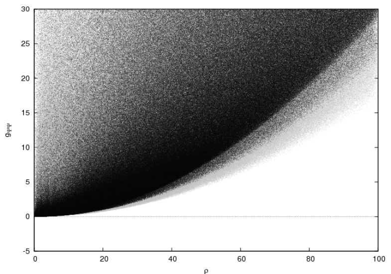
Figure B.1: The values of $g_{\psi\psi}$ as a function of $\rho$ at the end of the minimization procedure; this occurs either at local minima, or at points where the minimizing sequence leads to coalescing $a_{i}$’s. The three samples a), b), c) are presented with different grey intensity (from low to high, respectively). The initial parameters $(z,d_{ij})$ for the minimization procedure were randomly chosen, uniformly distributed in the intervals a) $z\in(-150,301)$, $d_{ij}\in(0,50)$, b) $z\in(-150,226)$, $d_{ij}\in(0,25)$, c) $z\in(-150,166)$, $d_{ij}\in(0,5)$. For each sample, the minimum of $g_{\psi\psi}$ is proportional to $\rho^{2}$.

In Figure B.2 one observes a linear lower bound on $g_{\psi\psi}|_{\rho=0}$ for $z<a_{1}$, with a slope approximatively equal to $-2$ with our choice of scale $a_{5}-a_{1}=1$.

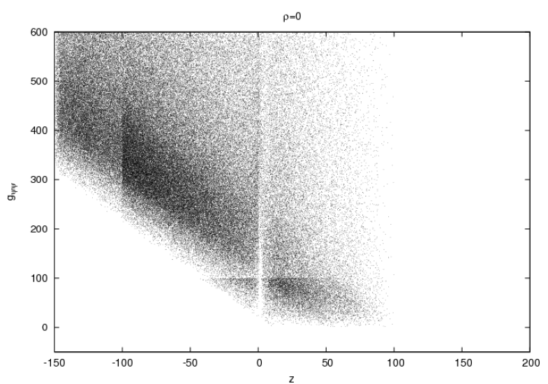
Figure B.2: The values of $g_{\psi\psi}$ for $\rho=0$ at the end of the minimization procedure; this occurs at points where the minimizing sequence leads to coalescing $a_{i}$’s. The initial parameters $(z,d_{ij})$ for the minimization procedure were randomly chosen, uniformly distributed in the intervals $z\in(-150,301)$, $d_{ij}\in(0,50)$.

The numerical results presented in this section support the hypothesis that $g_{\psi\psi}$ is never negative in the region of parameters of interest, vanishing only on the axis of rotation $\{\rho=0\;,\ z\geq a_{2}\}$.

Acknowledgements PTC acknowledges useful discussions with Christopher Hopper. We thank Marcus Ansorg, Henriette Elvang, Jörg Hennig and Pau Figueras for useful comments.

The research was partly carried out with the supercomputer “Deszno” purchased thanks to the financial support of the European Regional Development Fund in the framework of the Polish Innovation Economy Operational Program (contract no. POIG.02.01.00-12-023/08).

The main part of our calculations was carried out with Mathematica together with the xAct [8] package. We are grateful to José María Martín–García and Alfonso García–Parrado for sharing their Mathematica and xAct expertise.

References

- [1] J.M. Bardeen, Rapidly rotating stars, disks, and black holes, Black holes/Les astres occlus (École d’Été Phys. Théor., Les Houches, 1972), Gordon and Breach, New York, 1973, pp. 245–289. MR MR0465047 (57 #4960)
- [2] P.T. Chruściel and J. Cortier, On the geometry of Emparan-Reall black rings, (2008), arXiv:0807.2309 [gr-qc].
- [3] P.T. Chruściel and L. Nguyen, Ghost points in inverse scattering constructions of stationary Einstein metrics, (2010).
- [4] H. Elvang and P. Figueras, Black Saturn, Jour. High Energy Phys. (2007), 050, 48 pp. (electronic), arXiv:hep-th/0701035. MR MR2318101
- [5] H. Elvang, P. Figueras, G.T. Horowitz, V. Hubeny, and M. Rangamani, On universality in ergoregion mergers, Class. Quantum Grav. 26 (2009), 085011, 34, arXiv:0810.2778 [gr-qc]. MR MR2524556
- [6] M. Galassi et al., GNU scientific library reference manual, 3rd ed., URL http://www.gnu.org/software/gsl.
- [7] J. Hennig, M. Ansorg, and C. Cederbaum, A universal inequality between the angular momentum and horizon area for axisymmetric and stationary black holes with surrounding matter, Class. Quantum Grav. 25 (2008), 162002, 8. MR MR2429717 (2009e:83092)
- [8] J.M. Martín-García, xAct: Efficient Tensor Computer Algebra, http://metric.iem.csic.es/Martin-Garcia/xAct.
- [9] R. Meinel, M. Ansorg, A. Kleinwächter, G. Neugebauer, and D. Petroff, Relativistic figures of equilibrium, Cambridge University Press, Cambridge, 2008. MR MR2441850 (2009g:83001)
- [10] A.A. Pomeransky, Complete integrability of higher-dimensional Einstein equations with additional symmetry, and rotating black holes, Phys. Rev. D73 (2006), 044004, arXiv:hep-th/0507250.
- [11] I. Rácz and R.M. Wald, Global extensions of space-times describing asymptotic final states of black holes, Class. Quantum Grav. 13 (1996), 539–552, arXiv:gr-qc/9507055. MR MR1385315 (97a:83071)