Optimal linear reconstruction of dark matter from halo catalogs

Abstract

We derive the weight function $w(M)$ to apply to dark-matter halos that minimizes the stochasticity between the weighted halo distribution and its underlying mass density field. The optimal $w(M)$ depends on the range of masses being used in the estimator. While the standard biased-Poisson model of the halo distribution predicts that bias weighting is optimal, the simple fact that the mass is comprised of halos implies that the optimal $w(M)$ will be a mixture of mass-weighting and bias-weighting. In $N$-body simulations, the Poisson estimator is up to $15\times$ noisier than the optimal. Implementation of the optimal weight yields significantly lower stochasticity than weighting halos by their mass, bias or equal weighting in most circumstances. Optimal weighting could make cosmological tests based on the matter power spectrum or cross-correlations much more powerful and/or cost-effective. A volume-limited measurement of the mass power spectrum at $k=0.2h/$Mpc over the entire $z<1$ universe could ideally be done using only 6 million redshifts of halos with mass $M>6\times 10^{13}h^{-1}M_{\odot}$ ($1\times 10^{13}$) at $z=0$ ($z=1$); this is $5\times$ fewer than the Poisson model predicts. Using halo occupancy distributions (HOD) we find that uniformly-weighted catalogs of luminous red galaxies require $\geq 3\times$ more redshifts than an optimally-weighted halo catalog to reconstruct the mass to the same accuracy. While the mean HODs of galaxies chosen to lie above a threshold luminosity are fortuitously very similar to the optimal $w(M)$, the stochasticity of the halo occupation degrades the mass estimator. Blue or emission-line galaxies are $\approx 100\times$ less efficient at reconstructing mass than an optimal weighting scheme. This suggests an efficient observational approach of identifying and weighting halos with a deep photo-z survey before conducting a spectroscopic survey. The optimal $w(M)$ and mass-estimator stochasticity predicted by the standard halo model for $M>10^{12}h^{-1}M_{\odot}$ are in reasonable agreement with our measurements, with the important exceptions that the halos must be assumed to be linearly biased samples of a “halo field” that is distinct from the mass field. Halo catalogs extending below $10^{12}h^{-1}M_{\odot}$ are more stochastic than the halo model predicts, suggesting that halo exclusion or other effects violate the assumption that halos sample this “halo field” via a Poisson process.

1 Introduction

One challenge in survey cosmology is to infer the true dark matter density field from observables, i.e. galaxies and galaxy clusters from galaxy surveys in the UV, visible, NIR, or radio, or galaxy clusters detected in X-ray or Sunyaev-Zeldovich (SZ) (Sunyaev & Zeldovich, 1972) surveys. All these observable populations, as well as their host dark matter halos, are biased tracers of their underlying dark matter. It is well know that the bias depends on halo properties, e.g. mass, formation time, etc. Moreover, the tracers are not deterministic, even on large scales, i.e. there is randomness in their clustering relative to that of the dark matter. Understanding such randomness, or stochasticity, is crucial for precise mass reconstruction and strengthening constraints in cosmological parameters from observables. In this work, we take a step back by assuming that we have perfect “observations” of dark matter halos and we aim to understand the stochasticity between halos and dark matter, and to develop an optimal mass estimator from halo catalogs.

The simplest assumption about the distribution of halos (or galaxies) is that they are drawn from the mass distribution in a biased Poisson process. This remains a common assumption, even though mass conservation arguments strongly suggest that this model cannot be correct (Sheth & Lemson, 1999). On the other hand, the consequences of the simple truism that the mass is the mass-weighted sum of all halos are only just beginning to be worked out. Abbas & Sheth (2007) showed that the usual expressions for halo bias (Mo & White, 1996; Sheth & Tormen, 2002) – which derive from the fact that halo abundances are top-heavy (i.e., massive halos are overrepresented) in denser regions—can also be derived from noting that a region which happens to have a top-heavy mass function will also be overdense.

The two approaches provide rather different prescriptions for how to construct an estimator of the mass field given a (subset of) the halos. The estimator assuming halos are Poisson sampled from the mass is considerably noisier than the one in which halos are mass weighted (Seljak et al., 2009; Hamaus et al., 2010, H10). In what follows, we will compare the differences between these two approaches, as well as provide a prescription for finding the optimal weight when only a subset of the halos are available.

In many respects, our approach is similar to that of H10. However, while they concentrate on the problem of writing a weighted halo field as a linear function of the mass field, we will focus on the inverse problem – that of writing the mass field as a weighted sum over the halos, and minimizing the RMS residual $E$ of the mass estimation.

This re-evaluation of the stochasticity in mass estimators is important for observational programs to constrain cosmological parameters via measurement of the mass power spectrum: the weighting scheme that minimizes stochasticity may suggest a change in targeting strategies for spectroscopic surveys, and will reduce the resources required for a volume-limited measure of the mass power spectrum. Other cosmological probes and tests of general relativity require cross-correlation of the estimated mass field with other observables such as gravitational lensing. These experiments should gain even more through the use of optimal mass reconstruction.

Section 2 describes previous work on how to use halos to estimate the mass distribution, when halos are a sampling of the mass field, and then contrasts these with the prescription which follows from assuming that the mass is mass-weighted halos. Section 3 presents various tests in simulations of this approach. Section 4 discusses implications of our findings, and a final section summarizes.

2 Bias, stochasticity, and linear estimators

Suppose we have two random variables, $m$ and $h$, both defined to have zero mean. We will later be interested in cases where these are the mass and halo density fluctuations in spatial cells, or Fourier coefficients of the fluctuation fields. Their covariance matrix can always be written as

$$\mbox{\bf C}=\left(\begin{array}[]{cc}P&rb_{\rm var}P\\ rb_{\rm var}P&b^{2}_{\rm var}P\end{array}\right).$$ (1)

$r$ is the correlation coefficient between $m$ and $h$, and $b_{\rm var}$ is called the “variance bias” by Dekel & Lahav (1999). Throughout this paper, the variable $P$ without subscript will mean the power in the mass distribution. We can quantify the error in any estimator $\hat{m}$ of the mass variable via

$$E^{2}\equiv\frac{\left\langle(m-\hat{m})^{2}\right\rangle}{\langle m\rangle^{2}}.$$ (2)

We will refer to $E$ as the stochasticity between the two variables. We can extend the definition to mean the RMS residual error after subtraction of any estimator $\hat{m}$ of the mass field. If we restrict the estimator $\hat{m}$ to be a linear function of $h$, i.e. $\hat{m}=wh$ for some weight $w$, then substitution into (2) yields

$$E^{2}=\left(1+w^{2}+b_{\rm var}^{2}-2wrb_{\rm var}\right).$$ (3)

$E$ is minimized at $w=r/b_{\rm var}$, which yields

$$E_{\rm opt}^{2}=1-r^{2}=\frac{|\mbox{\bf C}|}{\langle m^{2}\rangle\langle h^{2}\rangle}.$$ (4)

In many cases cosmological information is carried by the ratio $b$ between the two variables. If $m$ and $h$ are drawn from a bi-variate Gaussian distribution, then we can use the Fisher matrix formalism from Tegmark et al. (1997) to form the covariance matrix of the parameters $\{P,r,b_{\rm var}\}$ in C. If we draw $N_{m}$ pairs $(m,h)$ from the distribution, the uncertainties on $b_{\rm var}$ and $P$ after marginalization over other parameters are

$$\frac{\sigma_{P}}{P} = \sqrt{\frac{2}{N_{m}}}$$ (5)

$$\frac{\sigma_{b_{\rm var}}}{b_{\rm var}} = \sqrt{\frac{1-r^{2}}{N_{m}}}=\frac{E_{\rm opt}}{\sqrt{N_{m}}}=\sqrt{\frac{E_{\rm opt}^{2}}{2}}\,\frac{\sigma_{P}}{P}.$$ (6)

[See Sheth et al. (2005) for the real space version of this argument.] Note that the same stochasticity $E$ appears in $\sigma_{b}$. The appeal of cosmological tests based on ratios like $b_{\rm var}$ instead of power variables like $P$ is that the former require $E_{\rm opt}^{2}/2$ fewer mode measurements to reach the same accuracy and can hence be more powerful for a given survey. We will show below that this factor can reach $E_{\rm opt}^{2}/2<10^{-3}$ for estimation of the mass distribution from halo distributions.

In this paper we will adopt a covariance definition of bias for variable $h$ against $m$, in which the covariance matrix is written as

$$\mbox{\bf C}=\left(\begin{array}[]{cc}P&bP\\ bP&b^{2}P+{\cal N}\end{array}\right).$$ (7)

The “noise” component is ${\cal N}\geq 0$. Note that our $P$ is explicitly the mean power spectrum in realizations of the field $m$. We do not subtract shot noise.

From (4), the stochasticity of $h$ and $m$ is $E_{\rm opt}^{2}={\cal N}/(b^{2}P+{\cal N})=(1+b^{2}P/{\cal N})^{-1}$. If $h$ is a Fourier coefficient of the fluctuations in a biased Poisson sampling of the field $m$, with mean space density $n$, then ${\cal N}=1/n$. For any field $h$, therefore, we can define an effective space density via

$$(nb^{2})_{\rm eff}P=E_{\rm opt}^{-2}-1.$$ (8)

Recently, H10 concentrated on optimization of the quantity

$$\sigma_{w}^{2}\equiv\left\langle(\delta_{w}-\hat{\delta}_{w})^{2}\right\rangle,$$ (9)

where $\delta_{w}$ is a weighted halo map and $\hat{\delta}_{w}$ is a linear function of the mass fluctuations. Our approach (and motivation) is similar, although we focus on the inverse problem – that of writing the mass field as a weighted sum over the halos, and minimizing the RMS residual $E$ of the mass estimation.

2.1 Multidimensional linear estimators

Now consider attempting to estimate the mass fluctuation $\delta_{m}$ from the fluctuations $\delta_{i}$ of a collection of tracers, e.g. the fluctuations in bins of halo mass. We wish to construct an estimator $\hat{\delta}_{m}$ from a linearly weighted sum of the tracers:

$$\hat{\delta}_{m}\equiv\sum w_{i}\delta_{i}=\mbox{\boldmath$w$}\cdot\mbox{\boldmath$\delta$}.$$ (10)

With complete generality we can define the power $P$, the covariance bias vector ${\bf b}$ and the halo covariance matrix C via

$$\langle\delta_{m}^{2}\rangle = P,$$ (11)

$$\langle\delta_{m}\delta_{i}\rangle = b_{i}P,$$ (12)

$$\langle\delta_{i}\delta_{j}\rangle = C_{ij}.$$ (13)

Note that we have not subtracted a shot noise contribution from the halo variance. We will never subtract a Poisson shot noise term from the power spectra in this paper because it is our intention to test the simple assumptions about the nature of shot noise.

For any choice of weight vector $w$, the stochasticity of the resulting mass estimator is

$$E^{2}=1-2\mbox{\boldmath$b$}^{T}\mbox{\boldmath$w$}+\mbox{\boldmath$w$}^{T}\mbox{\bf C}\mbox{\boldmath$w$}/P.$$ (14)

The choice of $w$ that minimizes the stochasticity is

$$\mbox{\boldmath$w$}_{\rm opt}=\left(\mbox{\bf C}/P\right)^{-1}\mbox{\boldmath$b$},$$ (15)

making

$$E^{2}_{\rm opt}=1-\mbox{\boldmath$b$}^{T}\left(\mbox{\bf C}/P\right)^{-1}\mbox{\boldmath$b$}.$$ (16)

Note that this is the stochasticity-minimizing linear estimator quite generally, independent of any assumptions about Gaussianity or any details of the process generating the halo distributions. Linear estimators which minimize the RMS residual of a target are known as Wiener filters, and our form $\mbox{\boldmath$w$}=\mbox{\bf C}^{-1}\mbox{\boldmath$b$}$ is typical for such cases. Also it is generally true that the optimized mass estimator $\hat{\delta}_{\rm opt}$ will satisfy $\langle\hat{\delta}_{\rm opt}^{2}\rangle=\langle\hat{\delta}_{\rm opt}\delta_{m}\rangle$.

The weight Eq. (15) is proportional to that in eqn. (19) of H10, even though their derivation assumes Gaussianity and is not based on minimizing the stochasticity $E$.

2.2 Principal components

Bonoli & Pen (2009) investigate the stochasticity of the halo field with respect to the matter by taking the weight function to be the first (or higher) principal component (PC) of the halo covariance matrix C. In other words the weight $w$ is the eigenvector of C having the largest eigenvalue. If the $\delta_{i}$ are rotated into the principal components, then the matrix C becomes diagonal. If principal component $j$ has correlation coefficient $r_{j}$ with respect to the matter, then it is easy to see that

$$E^{2}_{\rm opt}=1-\sum_{j}r_{j}^{2}.$$ (17)

Hence a drawback of PC weighting is that the stochasticity of the first principal component (PC1) achieves the optimally low value only if no other PC’s correlate with the mass. Bonoli & Pen (2009) show that this is a good approximation only on the largest scales.

Another issue with PC weighting is that it is not stable to re-binning of the halo population. For example, when the halos occupy the mass distribution with a Poisson process, the bins must be chosen with equal $n_{i}$ in order for the first PC to dominate the correlation with the mass (as was done by H10). The optimal weighting Eq. (30) shown later in our paper is recovered only in the limit of vanishing shot noise, $n_{i}P\rightarrow\infty$. Since PC weighting is binning-dependent and non-optimal, we will not focus on it.

H10 find that the optimal weight vector is very close to the weakest principal component of the “shot noise matrix” $\mbox{\bf C}-\mbox{\boldmath$b$}P\mbox{\boldmath$b$}^{T}$ when the halos are binned in equal numbers. This is intriguing since there is no algebraic requirement for the correspondence.

2.3 Mass as mass-weighted halos

2.3.1 Mass completeness relation

If we partition all of the mass into halos, i.e. extend the halo catalog to zero mass, then the mass distribution is the mass-weighted sum of the halo distributions (e.g., Abbas & Sheth, 2007). Hence we will obtain a perfect $E=0$ estimator of mass if we weight each halo bin by the fraction of the total mass it holds:

$$\eta_{i}=\frac{n_{i}m_{i}}{\sum_{i}n_{i}m_{i}}=\frac{n_{i}m_{i}}{\bar{\rho}},$$ (18)

where $m_{i}$ is the mean mass of halos in bin $i$ and $\bar{\rho}$ is the overall mean density. Since $E=0$ is clearly the optimal result, it is mass weighting which is optimal. If, on the other hand, halos occupy the mass distribution via a biased Poisson process, it is optimal to weight halos by their bias factors (we show this explicitly below). Therefore, the biased Poisson model cannot be correct in the limit that the halo catalog includes all of the mass.

The simple truism that the mass is the mass-weighted sum of all halos suggests that the optimal estimator will tend toward mass weighting as we include lower-mass halos. Park & Choi (2009) note in N-body simulations that mass-weighted halo catalogs attain lower stochasticity than uniform weighting. Seljak et al. (2009) show that weighting by mass (or other functions of mass) produces significantly lower stochasticity than expected from Poisson shot noise. H10 derived that weight function which optimizes $\sigma_{w}^{2}$. We derive the analogous optimal weight for $E$.

2.3.2 Mass estimation with incomplete halo catalogs

Suppose we are given a list of halo masses and positions. Suppose that this list is complete down to some limiting mass $m_{d}$. We can assign the remainder of the mass to a “dust bin,” which contains the fraction $\eta_{d}=1-\sum\eta_{i}$ of mass that is not in the halos.

If $\delta_{d}$ is the relative density fluctuation field of the mass in the dust bin, we can define the power of the dust field as

$$P_{d}=\langle\delta_{d}^{2}\rangle$$ (19)

and a bias vector $\mbox{\boldmath$c$}_{d}$ between halos and dust by

$$c_{di}=\frac{C_{di}}{P_{d}}=\frac{\langle\delta_{d}\delta_{i}\rangle}{P_{d}}.$$ (20)

Because

$$\delta_{m}\equiv\eta_{d}\delta_{d}+\sum\eta_{i}\delta_{i},$$ (21)

the bias and optimal weighting for the halo bins against the mass are:

$$P = \eta_{d}^{2}P_{d}+2\eta_{d}P_{d}\mbox{\boldmath$\eta$}^{T}\mbox{\boldmath$c$}_{d}+\mbox{\boldmath$\eta$}^{T}\mbox{\bf C}\mbox{\boldmath$\eta$},$$ (22)

$$P\mbox{\boldmath$b$} = \eta_{d}P_{d}\mbox{\boldmath$c$}_{d}+\mbox{\bf C}\mbox{\boldmath$\eta$},$$ (23)

$$\mbox{\boldmath$w$}_{\rm opt} = \mbox{\boldmath$\eta$}+(\eta_{d}P_{d})\mbox{\bf C}^{-1}\mbox{\boldmath$c$}_{d},$$ (24)

$$E^{2}_{\rm opt} = \frac{\eta_{d}^{2}}{P/P_{d}}\,\left(1-\mbox{\boldmath$c$}_{d}^{T}\mbox{\bf C}^{-1}\mbox{\boldmath$c$}_{d}P_{d}\right).$$ (25)

In this formulation it is apparent that as our halo catalog extends to lower masses and $\eta_{d}\rightarrow 0$, the optimal weight $\mbox{\boldmath$w$}_{\rm opt}\rightarrow\mbox{\boldmath$\eta$}$, i.e. mass weighting, and $E^{2}\rightarrow 0$. The further question of interest for finite $\eta_{d}$ is: How well do the known halo fluctuations $\delta_{i}$ predict the dust bin density $\delta_{d}$?

2.4 Sampling Models

So far the analysis has been completely general as to the generation of the mass field and the designation of halos within it. Now we examine models for the relation between halos and mass.

The most common assumption about the distribution of halos (or galaxies) is that they are drawn from the mass distribution in a biased Poisson process. If we are examining the Fourier coefficients of the mass and halo distributions, the biased Poisson model can be broken down into three assumptions:

1. The halos are a linearly biased sampling of some continuous “halo field” $\delta_{h}$ with power $\langle\delta_{h}^{2}\rangle=P_{h}$, via some stochastic process that has no spatial correlations. Then the covariance matrix of halo bins can be written as a rank-one matrix plus a diagonal “shot noise:”

   C $$= P_{h}\mbox{\boldmath$v$}\mbox{\boldmath$v$}^{T}+{\rm diag}(\mbox{\boldmath${\cal N}$}),$$ (26)

   $${\cal N}_{i} = f_{i}/n_{i}.$$ (27)

   Here $f_{i}>0$ is a “clump size” factor relating the noise ${\cal N}_{i}$ in bin $i$ to the space density $n_{i}$ of sources in the bin. Halos in bin $i$ are drawn with bias $v_{i}$ from the halo field.

2. The halos are placed by a Poisson process so that $f_{i}=1$.

3. We identify the halo field $\delta_{h}$ with the mass $\delta_{m}$ such that $P_{h}=P$ and $\mbox{\boldmath$v$}=\mbox{\boldmath$b$}$. In this case $\mbox{\bf C}=P\mbox{\boldmath$b$}\mbox{\boldmath$b$}^{T}+{\rm diag}(1/n_{i})$.

Assumption (iii) of the biased-Poisson model has been noted to be inconsistent with the assumption that the halo catalog can be extended to comprise all of the mass. We will therefore consider models in which assumption (i) holds without (iii), such that the halos sample a field that is distinct from the mass distribution. We will take care therefore to distinguish $v$, the bias of the halos with respect to the halo field $\delta_{h}$, from $b$, which we always define via the covariance with mass as per (7).

The assumptions that halos are linearly biased, and that the halo generating process has no spatial correlations are idealizations: in fact, halos in simulations do not overlap (almost by definition), and their bias is non-linear. We will return to the limits of these assumptions later.

When C takes the form (26), two things are of note: first, this description is stable under re-binning of the halos in the limit of narrow bins. More specifically, if $v_{i}$ and $f_{i}$ are slowly-varying functions of the mass $m_{i}$ of halos in bin $i$, then the $v_{i}$ and $f_{i}$ do not change if two adjacent bins are merged. In other words we can write functions $v(m)$ and $f(m)$, and all of our linear-algebra formulations can be carried over into integrals over halo mass $m$. The second useful fact about (26) is that it can be inverted analytically using the Sherman-Morrison formula:

$$P_{h}\left(\mbox{\bf C}^{-1}\right)_{ij} = x_{i}\delta_{ij}-\frac{x_{i}v_{i}x_{j}v_{j}}{1+\sum x_{i}v_{i}^{2}}$$ (28)

$$x_{i} \equiv P_{h}/{\cal N}_{i}=n_{i}P_{h}/f_{i}.$$ (29)

When all three conditions of the biased-Poisson model are met, the optimal weight function and stochasticity are found simply from (15) and (28):

$$\frac{w_{{\rm opt},i}}{n_{i}} = b_{i}\frac{P}{1+\sum n_{i}b_{i}^{2}P},$$ (30)

$$E^{2}_{\rm opt} = \left(1+\sum n_{i}b_{i}^{2}P\right)^{-1},$$ (31)

$$(nb^{2})_{\rm eff} = \sum n_{i}b_{i}^{2}.$$ (32)

This recovers the result from Percival et al. (2004) that the optimal linear mass estimator in a Poisson model weights each halo by its bias $b_{i}$ (times a mass-independent factor), and the stochasticity of the estimator is determined by $\sum n_{i}b_{i}^{2}P$. Conveniently the weights scale with the bias, independent of the range of halo masses included in the estimator. This property does not hold for more general forms of C and $b$, e.g. it fails when $\mbox{\boldmath$v$}\neq\mbox{\boldmath$b$}$ and condition (iii) is violated.

In this paper we will not assume that the halos occupy the matter distribution via a biased Poisson process. We will examine the C matrix for halos in numerical simulations, examine what if any of the three biased-Poisson conditions actually holds, and then use the general formulae (15) and (16) to find how the optimal stochasticity differs from the Poisson predictions.

2.4.1 General sampling model

We now examine the case where all halos, and the dust, are indeed placed by a local process that is biased relative to some halo field $\delta_{h}$, so assumption (i) holds but (ii) and (iii) are not assumed. This model illustrates the difference between the halo field that is sampled and the mass field that the halos comprise. The two fields cannot be equivalent, even in the linear regime. In §3.7, we examine whether halo covariance matrices measured in simulations are in fact consistent with this sampling model.

If all the halos and dust are placed in this halo field by independent processes, and we define a weighted field

$$\delta_{v}\equiv\frac{\sum_{i}n_{i}v_{i}\delta_{i}}{\sum_{i}n_{i}v_{i}},$$ (33)

then the covariances between the dust, the halo bins, and $\delta_{v}$ are

C $$= \mbox{\boldmath$v$}\mbox{\boldmath$v$}^{T}P_{h}+{\rm diag}(f_{i}/n_{i})$$ (34)

$$P_{d}=C_{dd} = v_{d}^{2}P_{h}+{\cal N}_{d}$$ (35)

$$C_{di} = v_{d}v_{i}P_{h}$$ (36)

$$C_{dv} = v_{d}\frac{\sum_{i}n_{i}v_{i}^{2}}{\sum_{i}n_{i}v_{i}}P_{h}$$ (37)

$$C_{vv} = \left(\frac{\sum_{i}n_{i}v_{i}^{2}}{\sum_{i}n_{i}v_{i}}\right)^{2}P_{h}+\frac{\sum_{i}n_{i}v_{i}^{2}f_{i}}{(\sum_{i}n_{i}v_{i})^{2}}$$ (38)

We have freedom in setting the normalization of $v_{d}$ and $v$ which we do by requiring

$$\eta_{d}v_{d}+\mbox{\boldmath$\eta$}\cdot\mbox{\boldmath$v$}=1.$$ (39)

In this case the mass, which is the sum of halo and dust densities, has power

$$P=C_{mm} = P_{h}+\eta_{d}^{2}{\cal N}_{d}+\sum\eta_{i}^{2}f_{i}/n_{i}$$ (40)

$$= P_{h}+\eta_{d}^{2}{\cal N}_{d}+(1-\eta_{d})^{2}\langle fm^{2}\rangle/\langle m\rangle^{2}$$ (41)

$$\equiv P_{h}+{\cal N}_{m}.$$ (42)

The angle brackets denote number-weighted averages over the halo population, and the final expression defines ${\cal N}_{m}$. We see that when the mass field is a sampled realization of the halo field, then $P\equiv C_{mm}$ is larger than $P_{h}$ by terms representing the sampling shot noise.

The bias $b$ of the halo mass bins relative to the mass distribution will not in general equal the bias $v$ with respect to the halo field. Since $b_{i}P=\langle\delta_{i}\delta_{m}\rangle,$ we can expand $\delta_{m}$ using (21), and use the C elements above, to derive

$$\mbox{\boldmath$b$}=\frac{\mbox{\boldmath$v$}+{\rm diag}(m_{i}f_{i}/P_{h}\bar{\rho})}{P/P_{h}}.$$ (43)

Formally, only $v_{i}\propto f_{i}m_{i}$ will yield $\mbox{\boldmath$b$}\propto\mbox{\boldmath$v$}$. In general, $b_{i}>v_{i}$ at sufficiently large masses, and $b_{i}<v_{i}$ at lower masses. Equality is at $m_{i}=b_{i}{\cal N}_{m}\bar{\rho}$, which occurs for $z=0$ at $\sim 10^{14}h^{-1}M_{\odot}$. In a $\Lambda$CDM model, the $b=v$ crossover will occur for halos with $b\approx 1.6$ for a wide range of redshifts. We can also solve for the weight vector of the optimal linear mass estimator:

$$\frac{w_{{\rm opt},i}}{n_{i}}=\frac{m_{i}}{\bar{\rho}}+\eta_{d}v_{d}\,(v_{i}/f_{i})\,P_{h}\,E^{2}_{\rm pois},$$ (44)

where we have set $E^{2}_{\rm pois}\equiv(1+\sum_{j}n_{j}v_{j}^{2}P_{h}/f_{j})^{-1}$; the sum over $j$ is over the halo bins in the catalog. $E^{2}_{\rm pois}$ describes the fidelity with which the halos can estimate the halo field, as opposed to the mass field. Notice that the first term is the mass weighting $(w\propto m)$, and the second correction term has the same form as that for the standard Poisson model $(w\propto v)$, but its importance depends on the mass fraction in dust, and how it clusters. Thus, equation (44) is a weighted sum of equations (18) and (30). As the halo catalog comprises more of the total mass, $\eta_{d}\rightarrow 0$, and mass weighting becomes optimal.

If we define $\delta_{\rm opt}\equiv\sum_{i}w_{{\rm opt},i}\delta_{i}$, then the optimized stochasticity is

$$E^{2}_{\rm opt} = 1-\frac{\langle\delta_{\rm opt}\delta_{m}\rangle^{2}}{\langle\delta_{\rm opt}^{2}\rangle\langle\delta_{m}^{2}\rangle}=1-\frac{\langle\delta_{\rm opt}\delta_{m}\rangle}{\langle\delta_{m}^{2}\rangle}$$ (45)

$$= \frac{\eta_{d}^{2}C_{dd}}{C_{mm}}\,\left(1-\frac{C_{dv}^{2}}{C_{dd}C_{vv}}\right)$$ (46)

$$= \frac{\eta_{d}^{2}}{P_{m}}\left({\cal N}_{d}+v_{d}^{2}P_{h}\,E^{2}_{\rm pois}\right).$$ (47)

We have written the second equality explicitly to show that $E_{\rm opt}$ makes physical sense: since $\eta_{d}^{2}C_{dd}/C_{mm}$ is the fraction of the total $C_{mm}$ that is in dust, the stochasticity is the yet smaller portion of this dust power that cannot be recovered via the correlation between the dust and the bias weighted halos.

The final expression shows that $E_{\rm opt}\to 0$ as the mass fraction in dust $\eta_{d}\to 0$, as it should. When $P_{h}\to 0$, then $E_{\rm opt}^{2}\to\eta_{d}^{2}{\cal N}_{d}/{\cal N}_{m}$: in this limit, the stochasticity is determined by the fraction of the noise term ${\cal N}_{m}$ which is contributed by the dust. The opposite limit is when $P_{h}\gg{\cal N}_{m}$, where $P\approx P_{h}$ and $E_{\rm opt}\to\eta_{d}v_{d}E_{\rm pois}$. Since $\eta_{d}v_{d}<1$, this is why the optimal stochasticity can be substantially smaller than in the Poisson model.

The optimized weights and relations between $b$ and $v$ are similar to what H10 found in their analysis of $\sigma_{w}$. E.g., our equation (43) reduces to their equation (41) upon taking $f_{i}\rightarrow 1$, $P_{h}\rightarrow P_{\rm lin}$, and $v_{i}\rightarrow b_{i}$. In the discussion following their Eq. (36), H10 note that their optimal weight is a linear combination of mass and bias weighting, a point they make again with their Eq. (49). But our expression for the relative contributions of these two weights is substantially more transparent than theirs. For instance, our formulation shows that this factor is, in fact, the one associated with the usual Poisson-sampling model, times a factor which accounts for the dust – this is not obvious from their expressions.

2.5 The halo model description

The halo model is a specific case of the sampling model in the previous section. The halo model is particularly well-suited to describing the effect of weighting halos (Sheth, 2005); it predicts not only C, but also the dust-bin quantities like ${\cal N}_{d}$ and $P_{d}$ which are not observable and were left unspecified in the previous section. Hence the halo model allows an estimate of the stochasticity $E_{w}$ associated with any weight function $w$ applied to the halos, so it can be used to estimate $E_{\rm opt}$. (In the context of the optimal weight discussed earlier, it provides a prescription for the effect of bias weighting halos.)

In what follows, we will explicitly set $f=1$; comparison of the predictions of this calculation with the measurements in simulations provides a measure of the accuracy of this assumption. In particular, if we define

$$n_{w} = \int_{m_{d}}^{\infty}dm\,\frac{dn}{dm}\,w(m),$$ (48)

$${\cal N}_{w} = \int_{m_{d}}^{\infty}dm\,\frac{dn}{dm}\,\frac{w^{2}(m)}{n_{w}^{2}},$$ (49)

$${\cal N}_{\times} = \int_{m_{d}}^{\infty}dm\,\frac{dn}{dm}\,\frac{m\,u(k|m)}{\bar{\rho}}\,\frac{w(m)}{n_{w}},$$ (50)

$${\cal N}_{m} = \int_{0}^{\infty}dm\,\frac{dn}{dm}\,\frac{m^{2}\,|u(k|m)|^{2}}{\bar{\rho}^{2}}$$ (51)

then

$$C_{ww} = v_{w}^{2}\,P_{h}(k)+{\cal N}_{w},$$ (52)

$$C_{wm} = v_{w}\,P_{h}(k)+{\cal N}_{\times},$$ (53)

where

$$v_{w}=\int_{m_{d}}^{\infty}dm\,\frac{dn}{dm}\,\frac{w(m)}{n_{w}}\,v(m).$$ (54)

Here $v(m)$ is the bias with respect to $P_{h}(k)$; it is related to the bias $b(m)$ with respect to the mass field by equation (43). The factor $u(k|m)$ in the expressions above represents the fact that halo catalog is treated as if all mass is concentrated at the center of mass, but real halo mass is smeared in a density profile: $u$ is the Fourier transform of the density profile, normalized so that $u\to 1$ as $k\to 0$.

Strictly speaking, this writing of the halo model is not quite correct, because halos of a given mass may have a range of density profiles, i.e. $u$ is not the same for all halos, and stochasticity in $u$ will contribute to $E$. If we use the mean $u$ for a given $k$ in the expressions above, and define $\sigma_{u}^{2}(k|m)\equiv\langle|u^{2}|\rangle-\langle u\rangle^{2}$, then then the scatter in profile shapes will contribute an additional term

$${\cal N}_{m}\rightarrow{\cal N}_{m}+\int dm\frac{dn}{dm}\sigma_{u}^{2}(k|m)\left(\frac{m}{\bar{\rho}}\right)^{2}.$$ (55)

We expect this additional term to be unimportant at the scales $k<0.1h\,{\rm Mpc}^{-1}$ that are of most interest for cosmology Sheth & Jain (2003). Section 3.6 shows that this is indeed the case. However, this term grows as $k^{4}$, so it could dominate the stochasticity at higher $k$.

The results of the previous section suggest that an optimal linear reconstruction of the mass can be obtained if we use equation (44) for the weight function. If we set $f_{i}=1$, then

$$w_{\rm opt}(m)=\frac{m\,u(k|m)}{\bar{\rho}}+F_{v}\,\frac{v(m)\,P_{h}(k)}{1+(nv^{2})_{h}P_{h}(k)},$$ (56)

where

$$F_{v} = 1-\int_{m_{d}}^{\infty}dm\,\frac{dn}{dm}\frac{m\,u(k|m)}{\bar{\rho}}\,v(m)$$ (57)

$$(nv^{2})_{h} = \int_{m_{d}}^{\infty}dm\,\frac{dn}{dm}\,v^{2}(m).$$ (58)

This makes the stochasticity

$$E_{w_{\rm opt}}^{2}=1-\frac{C_{wm}^{2}}{C_{mm}C_{ww}}=1-\frac{n_{w}\,C_{wm}}{C_{mm}}$$ (59)

equal the expression given in equation (45). (Note that, for these choices of $w$ and $v$, $n_{w}^{2}\,C_{ww}=n_{w}C_{wm}$, and $E_{w_{\rm opt}}^{2}$ is independent of $u$.)

Thus, we can use the halo model to estimate the stochasticity $E_{w}^{2}$ associated with the weight $w$ of equation (56) as follows. We can measure the mass power spectrum $P$ and the covariance bias $b(m)$ in the simulations, and then use equation (43) to infer $v(m)P_{h}$. We then use the halo model to estimate ${\cal N}_{m}$, which we subtract from the measured $P$ to get $P_{h}$, and hence $v(m)$. These can then be used to estimate $F_{\nu}$ and $(nv^{2})_{h}$ by summing over the halos. The halo model can also be used to estimate ${\cal N}_{m}$; by directly measuring the component of this that comes from the halos in the sample, one can determine ${\cal N}_{d}$ and so estimate $E_{w}$. In the following section, we will compare this Poisson sampled and mass-weighted halo model for $E_{w}$ with the optimal stochasticity in simulations.

2.5.1 Halo exclusion and other subtleties

We could have made heavier use of the halo model as follows. The usual implementation (Sheth, 2005) replaces $v(m)\,P_{h}\to b_{\rm pbs}(m)\,P_{m}$, where $b_{\rm pbs}(m)$ is the peak background split bias (Bardeen et al., 1986; Cole & Kaiser, 1989; Mo & White, 1996; Sheth & Tormen, 1999, e.g.), and $P_{m}$ is the power spectrum of the mass, usually approximated by $P_{\rm lin}$ at small $k$. H10 make this same assumption in their halo model of $\sigma_{w}$. We will show later that $b_{\rm pbs}(m)$ appears to be closer to $v(m)=(C_{hm}-{\cal N}_{\times})/(C_{mm}-{\cal N}_{m})$ than it is to $b(m)=C_{hm}/C_{mm}$. However, note that our discussion indicates that $P_{h}$ is not to be identified with the mass power spectrum and $v(m)$ is not the same as the linear bias factor between the halo and mass fields. This is one reason why our construction of the halo model above was slightly different from standard. In particular, we did not begin from the mass field $\delta_{m}$, and immediately set $P_{h}=P_{m}$, as is usually done. Rather, we framed our discussion in terms of the field $\delta_{h}$, and weighted samplings of it. Because we assumed that halos were linearly biased Poisson samplings of this field, we explicitly ignored the fact that, in reality halos are spatially exclusive, and the sampling function is not just a linear function of the mass. The exclusion property means that the assumption that the halos are obtained from independent sampling processes for every mass bin cannot be correct. Indeed, in the sampling algorithm described in (Sheth & Lemson, 1999), this lack of independence appears explicitly – and it also contributes to the non-linearity of the bias relation (see their equation 17). [For more recent discussion of the effects of halo exclusion and non-linear bias on $P_{m}$, and another way of seeing why exclusion alone can produce effects which appear as scale dependent non-linear bias, see Smith et al. (2007).] As we shall see, our neglect of these effects sets a limit to the accuracy of our approach (e.g., the contribution to the stochasticity which comes from bias-weighting the halos may not be optimal).

2.5.2 Halo-mass-dependent selection function

The results above assume that all halos above a sharp threshold in mass are observed. If the threshold is not sharp, but is a function of mass, $0\leq p(m)\leq 1$, then it is straightforward to verify that equation (56) remains the optimal weight, provided that, in the previous expressions for $C_{ww}$, $C_{wm}$, $F_{v}$ and $(nv^{2})_{h}$ (but not ${\cal N}_{m}$, of course), all occurrences of $(dn/dm)$ are replaced by $(dn/dm)\,p(m)$. As a result, the sub-sampling decreases $n_{w}C_{wm}$; since $C_{mm}$ does not change (of course), the sub-sampling degrades (i.e., increases) $E$.

Table 1: Basic parameters used in the Millennium and NYU simulations. $\epsilon$ is the Plummer-equivalent comoving softening length of the gravitational force; $N_{\rm re}$ is the number of realizations for each simulation; $z_{\rm start}$ is the starting redshift for the simulation.

Name	$N_{p}$	$M_{p}$	$L_{box}$	$\epsilon$	$\Omega_{m}$	$\Omega_{\Lambda}$	$\Omega_{b}$	$\sigma_{8}$	$n_{s}$	$H_{0}$	$z_{start}$	$N_{re}$
Millennium	$2160^{3}$	$8.6\times 10^{8}~{}h^{-1}M_{\odot}$	500 $h^{-1}$Mpc	5$h^{-1}$kpc	0.25	0.75	0.045	0.9	1	73	127	1
NYU	$640^{3}$	$6\times 10^{11}~{}h^{-1}M_{\odot}$	1280 $h^{-1}$Mpc	20$h^{-1}$kpc	0.27	0.73	0.046	0.9	1	72	50	49

3 Optimal weights and mass estimators from simulations

3.1 Simulations

In this section we use N-body simulations to find optimal mass-estimation weights for halos binned by mass (rather than, e.g., angular momentum, axis ratio, formation time or concentration). We show the stochasticity that results from applying the optimal weights and compare to common sub-optimal choices.

For purposes of exploration, we wish to have a wide range of halo masses, while still having good statistics for large halos and large-scale modes. For the first purpose, we use the Millennium simulation (Springel et al., 2005), which resolves halos down to $\sim 10^{10}h^{-1}M_{\odot}$. For the second, we use the suite of 49 cosmological dark matter “NYU” simulations described in Manera et al. (2010), which have a total volume $800\times$ larger than the Millennium, but the minimum resolved halo mass is $1000\times$ larger. The simulations assume very similar $\Lambda$CDM cosmological models and were carried on using the same GADGET-2 code (Springel, 2005). Table 1 provides details of the basic simulation parameters.

The initial power spectrum was generated by CMBFAST (Seljak & Zaldarriaga, 1996). The initial density field of the Millennium simulation was realized by perturbing a homogeneous, glass-like particle distribution with a Gaussian random realization of the initial power spectrum (White, 1996), while the NYU simulations use an algorithm motivated by Second Order Lagrangian Perturbation Theory (Scoccimarro, 1998). Dark matter halos with at least 20 particles are identified in both simulations using the friends-of-friends (FOF) group finder with a linking length of $0.2$ times the mean particle separation (Davis et al., 1985). The lowest mass halo of the two simulations that we use are $1.7\times 10^{10}h^{-1}M_{\odot}$ and $1.0\times 10^{13}h^{-1}M_{\odot}$ respectively. The Millennium simulation has $\approx 1.8\times 10^{7}$ halos at at $z=0$, $z=0.5$ and $z=1$ while the NYU simulations have $\sim 4.3\times 10^{7}$, $3.5\times 10^{7}$ and $2.5\times 10^{7}$ halos in each of these redshift slices. For a more detailed analysis of the halo mass function and bias factors in these simulations, see Springel et al. (2005) and Manera et al. (2010).

Figure 1: The weight function for optimal reconstruction of the mass field on the scale $k=0.1h$Mpc^-1 at $z=0$ as a function of halo mass for the NYU simulations (left) and the Millennium simulation (right). The optimal weight depends on the minimum halo mass used in the reconstruction; solid lines (with arbitrary vertical offset), which are measured from simulations using Eq. (14), show this dependence. Dashed, dotted and blue curves show $w\propto M$, equation (56), and $w\propto b$, the latter being optimal if the Poisson model is correct. The optimal weighting steepens as $M_{\rm min}$ decreases, approaching $w\propto M$, although not exactly along the dotted curves predicted by our halo model implementation of the sampling model. Cyan and orange lines show the mean halo occupancy distributions (HODs) for blue galaxies and luminous red galaxies, respectively, in the low-$z$ SDSS spectroscopic sample.

Figure 2: Stochasticity $E$ of the estimators of the mass field derived from the weights shown in Figure 1, shown as a function of the minimum mass of halos in the catalog. The three panels show different $k$ values, all at $z=0$. In each panel, data at higher $M_{\rm min}$ are from the NYU simulations; lower $M_{\rm min}$ measurements are from the Millennium simulation. From the bottom up: black, purple, blue, and red solid curves show optimal, mass, bias and uniform weighting of the halos. Bias weighting would be optimal if the standard biased Poisson model were correct; it clearly is not. Dashed curve shows the halo model calculation of $E$ which assumes the mass is sum of halos that are Poisson-sampled from some halo field. The failure of the model at $M<10^{12}h^{-1}M_{\odot}$ is discussed in the text.

Figure 3: Unweighted (left) and optimally weighted (right) real-space halo density fluctuations $\delta_{h}$ versus dark matter density fluctuations $\delta_{m}$ smoothed by a spherical top-hat window function with the radius of $R=50h^{-1}Mph$. The three contour levels (0.1, 1, 10 shown in green, yellow, red) indicate the relative number density of data points in the $\delta_{m}$-$\delta_{h}$ plane. Diagnal black solid lines indicate $\delta_{h}=\delta_{m}$. Dash lines show the fitting results of the function $\delta_{h}=b_{0}+b_{1}\delta_{m}+b_{2}\delta_{m}^{2}$, with best-fit parameters shown in the figures. Top panels are results from the Millennium simulation with the mimimal halo mass of $M_{\rm min}=1.4\times 10^{10}h^{-1}M_{\odot}$. Bottom panels show results from the NYU simulations, with $M_{\rm min}=3.1\times 10^{13}h^{-1}M_{\odot}$.

3.2 Measuring power spectra and covariance matrices in simulations

We start our measurements by dividing halos into bins sorted by mass. The clustering of halos depends weakly on the halo mass when halo mass is low but increases rapidly with mass when $M>10^{13}~{}h^{-1}M_{\odot}$. Furthermore halo abundances drop sharply at high mass. As we do not want a wide range of masses within a single bin, we include fewer halos per bin at high masses.

We choose bins so that the number of halos in each decreases exponentially at high masses. The optimal weighting and stochasticity are robust to changes in the binning, as long as the function $b(M)$ is well sampled. We divide the halos into 10 bins for the NYU simulations, and use up to 30 bins for the Millennium simulation. We have tested that using more bins does not change our results.

Within each halo bin, we weight halos by their masses and assign them to a $N_{g}^{3}=256^{3}$ 3D mesh of cubic grid cells using the cloud-in-cell (CIC) assignment scheme (Hockney & Eastwood, 1981), i.e. we take the Fourier transform of the mass distribution within a halo bin. This is in anticipation of the result below that optimal weighting is closer to mass-weighting than number-weighting of halos. If the bins are narrow in mass, this choice of intra-bin weighting should have little effect, which we have verified.

We separately Fourier transform the overdensity field of each halo bin and the total mass distribution. We correct each Fourier mode for the convolution with the CIC window function by the operation:

$$\delta(\mbox{\boldmath$k$})=\delta(\mbox{\boldmath$k$})\,\left(\frac{\sin(x)}{x}\frac{\sin(y)}{y}\frac{\sin(z)}{z}\right)^{-2},$$ (60)

where $\{x,y,z\}=\{k_{x}L_{box}/2N_{g},k_{y}L_{box}/2N_{g},k_{z}L_{box}/2N_{g}\}$, and $N_{g}$ is the number of grid cells in each dimension. For each bin in $k$ we construct the covariance matrix of Fourier coefficients $C_{ij}(k)=\langle\delta_{i}(k)\,\delta_{j}(k)\rangle$, where $i$ and $j$ range over all halo bins, as well as the mass power $P=\langle\delta_{m}^{2}\rangle$, and hence the covariance biases $b$ of the halos against the mass. For the NYU simulations we average results from all 49 realizations to produce a mean covariance matrix.

Figure 4: Left: The effective source density $(nb^{2})_{\rm eff}$ of an optimally-weighted mass estimator is plotted (solid) vs $k$ for catalogs with a different halo mass cutoffs $M_{\rm min}$ as labeled. This measure of stochasticity is found to vary little with scale in the linear regime $k<0.1h$Mpc^-1. The dashed lines show the $nb^{2}$ expected via Equation (32) under a biased-Poisson model of galaxy stochasticity. The dotted line shows the $(nb^{2})_{\rm eff}$ required to attain $E=0.5$, i.e. a volume-limited power spectrum measurement. Right: For three different redshifts, we plot the optimal $(nb^{2})_{\rm eff}$ vs the minimum mass of the halo catalog used for mass reconstruction (solid lines). The dashed lines plot the $nb^{2}$ that we would expect if halos were a Poisson sampling of the mass distribution, as per Equation (32). Because halos comprise the mass rather than sampling the mass, the $(nb^{2})_{\rm eff}$ is up to $15\times$ higher, i.e. the mass estimator is less stochastic, than the Poisson model predicts.

3.3 Measured stochasticity and optimal weights

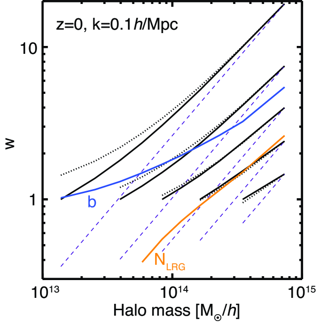
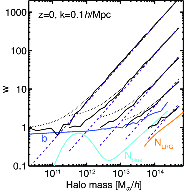
Figures 1 shows the optimal weights we derive from the simulations (black solid lines), and compares them with various functions of mass. Purple-dashed lines show $w\propto m$; blue curves show the bias weighting $w\propto b$ that would be appropriate if the standard biased-Poisson model were correct, and dotted curves show the optimal weight in equation (56) derived from the halo model of Section 2.5.

Clearly, neither $M$ nor $b$ are optimal weights. Indeed, the shape of $w_{\rm opt}(M)$ depends on the cut-off mass $M_{\rm min}$ of the halo catalogue. (This dependence follows that found by H10, in their study of $\sigma_{w}$.) When $M_{\rm min}<10^{13}~{}h^{-1}M_{\odot}$, the massive end of the $w_{\rm opt}(M)$ is close to mass weighting, as illustrated by the right-hand plot of Figures 1. When $M$ is close to $M_{\rm min}$, however, $w_{\rm opt}(M)$ is flatter than mass weighting. Moreover, the slope of $w_{\rm opt}(M)$ gets shallower as $M_{\rm min}$ increases, as shown in the left hand plot. Weighting halos by their masses is a poorer approximation to the optimal weight when $M_{\rm min}>10^{13}~{}h^{-1}M_{\odot}$. The halo model prediction of the optimal weight is generally in good agreement with the measurements. The agreement is not perfect, however, especially when $M$ approaches $M_{\rm min}$.

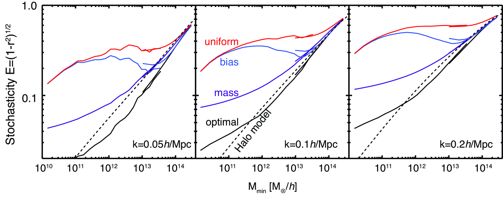
Figure 2 shows the stochasticity $E$ associated with these linear estimators $\hat{\delta}_{m}$ of the mass distribution, as a function of the minimum mass $M_{\rm min}$ of halos included in the sample. Black, purple, blue, and red solid curves show $E$ derived from optimal, mass, bias and uniform weighting of the halos. Weighting halos by their masses yields lower $E$ than bias weighting or equal weighting, but is significantly worse than the optimal when the halo catalog has $M_{\rm min}\approx 10^{13}h^{-1}M_{\odot}$ or lower. Bias weighting would be optimal if the standard biased Poisson model were correct, but is clearly far from optimal for halos in $N$-body simulations. The dashed curves show the halo model description of $E_{\rm opt}$ (equation 59). The model agrees with the measurements at $M_{\rm min}>10^{12}h^{-1}M_{\odot}$, but it does not predict the inflection we measure at smaller $M_{\rm min}$. We discuss this further in Section 3.6.

As an additional check of our numerical methods, we have verified that inclusion of the “dust bin” in the estimator leads to a perfect mass estimator ($E=0$) with optimal weights directly proportional to halo mass.

3.4 The scatter between the halo field and the mass field

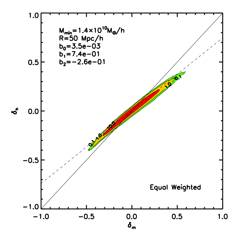
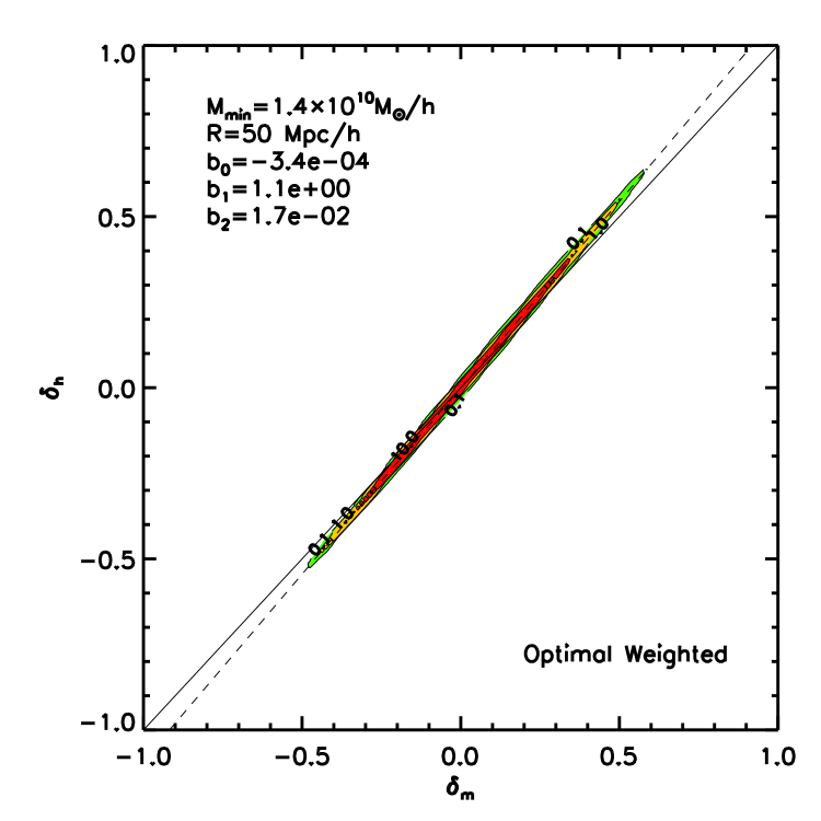
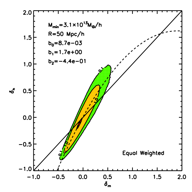
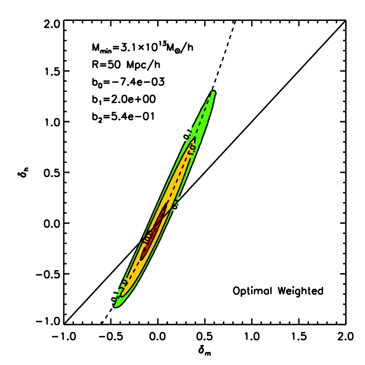
To illustrate the gain from applying the optimal weights, we show in Figure 3 the scatter between the fluctuations of the halo field $\delta_{m}$ and the mass density field $\delta_{m}$, before and after applying the optimal weights. Notice that $\delta_{h}$ and $\delta_{m}$ are both density contrasts in configuration space that are smoothed by the same spherical top-hat window function. We do the smoothing by multiplying the density contrasts in Fourier space with the Fourier transform of the window function, $\delta_{h,m}(k)=W_{R}(k)\delta_{h,m}(k)$, where $W_{R}(k)=3[\sin(kR)-kR\cos(kR)]/(kR)^{3}$ and $R$ is the radius of the window function. Then we Fourier transform back and get the smoothed $\delta_{h}$ and $\delta_{m}$.

We fit the scatter plots with the polynomial function $\delta_{h}=b_{0}+b_{1}\delta_{m}+b_{2}\delta_{m}^{2}$, to see if there is any indication of non-linear bias factor $b_{2}$. We usually find very small fitted values of $b_{2}$, especially for the optimal weighted cases. We also find an increase of $b_{2}$ value when increasing the low mass cut of the halo sample. In general, we see a significant improvment of applying the optimal weights, indicated by the shrinking of the scatter. This shows that the optimal weights indeed work well, without any higher-order bias correction.

3.5 Scale dependence of stochasticity

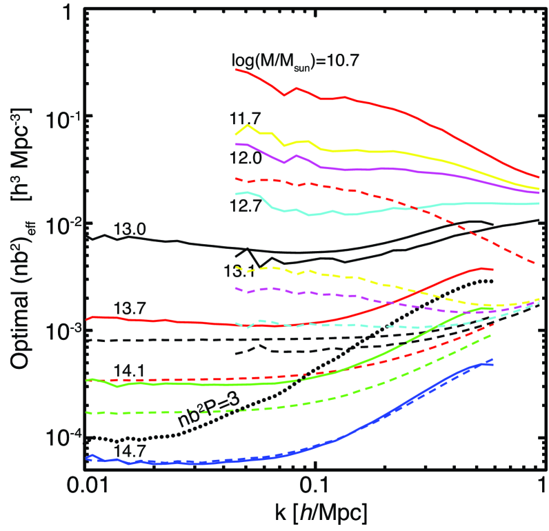
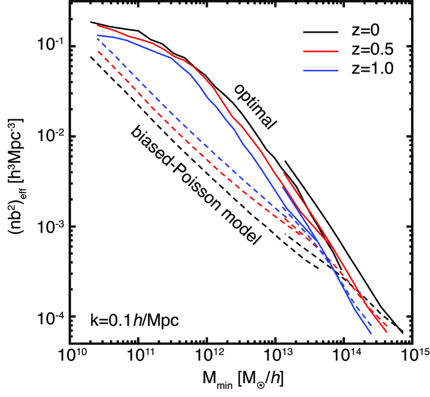
Figure 4 illustrates that the optimal $(nb^{2})_{\rm eff}$ is nearly independent of $k$ at fixed $M_{\rm min}$ in the linear regime, where $(nb^{2})_{\rm eff}$ is related to $E_{\rm opt}$ by equation (8). Since both $(nb^{2})_{\rm eff}$ and the Poisson prediction $(nb^{2})$ (the simple bias weighted sum over the halo population), are nearly constant across the linear regime, we compare them in the right panel of Figure 4 as a scale-independent measure of stochasticity. We find that at all redshifts and $M_{\rm min}$ values, the achievable $(nb^{2})_{\rm eff}$ is significantly better (higher) than would have been expected in the model where halos are a Poisson sampling of the mass. The ratio $(nb^{2})_{\rm eff}/(nb^{2})$ can be as high as $\approx 15$ for surveys of $M>10^{12}h^{-1}M_{\odot}$ halos at $z=0$. Even for surveys limited to massive clusters, $M_{\rm min}\approx 10^{14}h^{-1}M_{\odot}$, the effective source density of the optimal estimator is $\approx 2\times$ better than the Poisson model predicts.

3.6 Departures from the halo model

The dashed curve in Figure 2 plots the halo model prediction of the optimal $E$, which assumes the mass is comprised of halos that are Poisson-sampled from some halo field. The $E_{\rm opt}$ from simulations becomes shallower for $M_{\rm min}<10^{12}h^{-1}M_{\odot}$ where as the halo model does not. Either the halo model is not accurate at $M_{\rm min}<10^{12}h^{-1}M_{\odot}$, or there is some bias in the numerical estimation of $E_{\rm opt}$ from the simulation catalogs.

Calculating $E_{\rm opt}^{2}$ at $M_{\rm min}<10^{12}h^{-1}M_{\odot}$ sets heavy demands on the measurement of the covariances in the simulation, because $\mbox{\boldmath$b$}^{T}\mbox{\bf C}^{-1}\mbox{\boldmath$b$}$ must be calculated to a fractional accuracy of $E^{2}_{\rm opt}<10^{-3}$ in this regime. We have considered the possibility that $E_{\rm opt}$ levels off at small $M_{\rm min}$ because of discreteness effects. Specifically, in the simulations, mass comes in units of $m_{p}$, so the “dust” is not made of arbitrarily small halos. This makes ${\cal N}_{d}\to{\cal N}_{d}+1/n_{d}$ approximately. However, this additional factor is too small to explain the flattening we see. We have also verified that the plateau in $E_{\rm opt}$ is unaffected by the size of the bins in mass or $k$.

As noted earlier, the stochasticity $E$ will be degraded if halos of a given mass have varying internal structure, while we treat halos of a given mass as being identical point masses in the analysis. Within the halo model, the stochasticity adds to ${\cal N}_{m}$ as per (55). We test the magnitude of this effect by creating new halo overdensity maps from the full sample of $N$-body particles belonging to halos in each mass bin. These “true” halo mass maps are then used to create an optimal mass estimator. Figure 5 shows that the point-mass approximation has negligible impact on $E$ at $k<0.15h\,{\rm Mpc}^{-1}$, but at higher $k$ the mass estimator is increasingly degraded by the absence of information on the variability of internal structure of massive halos.

Figure 5: The optimal stochasticity $E$ as a function of wave-number $k$ from using all halos in the Millennium simulation is shown for two cases: the upper red curve treats each halo as a point mass, while the lower black curve uses the full spatial distribution of the particles comprising the mass of each halo. If the halo catalog does not contain information on the variability of internal halo structure at a given mass, it cannot fully map the mass distribution. This significantly degrades $E$ for $k>0.15h\,{\rm Mpc}^{-1}$, but does not explain the inflection in $E_{\rm opt}$ observed at $k\leq 0.1h\,{\rm Mpc}^{-1}$ for $M<10^{12}h^{-1}M_{\odot}$ in Figure 2.

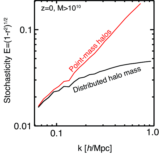
Even when we use the full halo mass distributions in our optimal estimator, the performance for $M_{\rm min}<10^{12}M_{\odot}$ remains worse than $E$ predicted by the halo model. It is possible that noise in $b$ and C  from having too few modes is compromising our measurements of $E_{\rm opt}$ in the Millennium simulation. This would most strongly affect the low-$k$ region where modes are scarcest, however the inflection does not exhibit this behavior.

We conclude that we have reached limits of the assumption that halos are a Poisson sampling of an underlying halo field. For $M\approx 10^{12}h^{-1}M_{\odot}$, $\eta_{d}\approx 0.66$ so the effects of exclusion/mass conservation are beginning to matter, so it is perhaps not surprising that the optimal mass reconstruction is poorly described by a model that presumes halos to be independently sampled from the halo field. We will defer to future work investigation of mass reconstruction in the presence of exclusion and other non-linear effects.

3.7 Explicit test of the sampling model

Are the observed covariance matrices of the halos consistent with their being stochastic discrete realizations of an underlying “halo field” $\delta_{h}$, the model of §2.4.1? We answer this question by asking how well the elements $C_{ij}$ of the simulations’ covariance matrices can be fit by appropriate values of the $v_{i}$ and $f_{i}$. We find the $\{v_{i},f_{i}\}$ which minimize the L2 norm of the residual to the model (34):

$$\lVert\delta\mbox{\bf C}\rVert_{2}\equiv\sum_{ij}\left(v_{i}v_{j}+\delta_{ij}f_{i}/n_{i}P-C_{ij}/P\right)^{2}.$$ (61)

(We use the mass power $P$ instead of $P_{h}$ in the fit, which slightly changes the values of $v_{i}$ and $f_{i}$ without affecting the quality of the fit.) Figure 6 plots the best-fitting values of $f_{i}$ and $v_{i}$ for each halo mass bin in the NYU simulations, along with the bias $b_{i}$. The fitted values of $f_{i}$ slightly exceed unity, but this is consistent with halos being a Poisson sampling ($f_{i}=1$) of a “halo field” because the mass-weighting within each halo bin will cause $f_{i}$ to rise slightly above unity, particularly in the most massive bin.

Figure 6: The best fit of the sampling model $C_{ij}=v_{i}v_{j}P+\delta_{ij}f_{i}/n_{i}$ to the $z=0$ halo catalog of the NYU simulation is shown as a function of $k$. The solid lines in the upper panel plot the bias $b_{i}$ of halos in each mass bin, while the dashed lines are the best-fit $v_{i}$ for each bin. Higher-mass bins have higher bias. Note that $v_{i}<b_{i}$ for massive halos, by an amount that grows at $k>0.1h\,{\rm Mpc}^{-1}$, but that $v_{i}>b_{i}$ at lower masses, as predicted. The lower panel shows the best-fit $f_{i}$. Poisson sampling would induce values slightly above $f_{i}=1$ because of the mass weighting within a halo bin, particularly for the most massive bin, as observed.

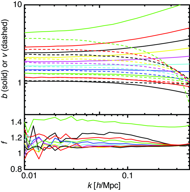
The fit to the sampling model does confirm a departure from the simple biased-Poisson model, however, in that the biases $v_{i}$ of the halos with respect to the parent halo field are not equal to the covariance biases $b_{i}$ with respect to the mass field. There is a divergence of $b$ from $v$ toward the trans-linear regime.

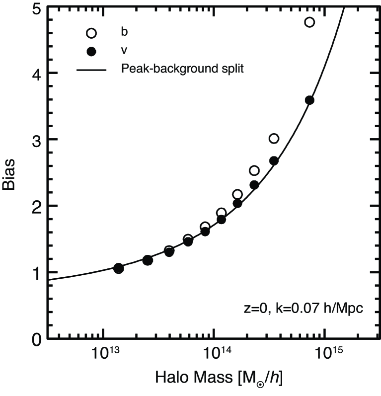
The peak-background split model yields an analytic prediction $b_{\rm pbs}$ for the bias of halos vs the underlying mass distribution. Figure 7 shows that for the NYU simulations, it is the bias $v$ of the halos vs the halo field $\delta_{h}$ that is best described by $b_{\rm pbs}$, not the bias $b$ of the halos vs the mass distribution. This observation should lead to a deeper theoretical understanding of the halo distribution. In particular, it may help resolve the discrepancy reported by Manera et al. (2010) between $b_{\rm pbs}$ and their measurements of halo bias, which were effectively what we call $b$, rather than $v$.

Figure 7: For the full NYU halo sample at $z=0$, we plot three types of bias. The open symbols are the covariance bias $b$ vs the mass distribution. The solid symbols are the bias $v$ vs the underlying continuum “halo field” $\delta_{h}$ in the sampling model that best fits the halo-mass covariance matrix. The curve is the analytic bias prediction of the peak-background split model.

The quality of the fit of the sampling model to the covariance matrix can be gauged by the ratio

$$R\equiv\frac{\sqrt{\lVert\delta\mbox{\bf C}\rVert}}{\lVert\mbox{\boldmath$v$}\rVert}.$$ (62)

This quantity measures the ratio of the RMS error in elements of C  to the RMS value of the model—excluding the diagonal elements, which are always perfectly fit by adjusting the $f_{i}$. For the NYU simulations at $z=0$ we find C well fit by this model: $0.01<R<0.035$ for all $k<0.25~{}h$Mpc^-1. For the bin at $k=0.07~{}h$Mpc^-1 in the NYU simulations, we would expect $R\approx 0.02$ from Gaussian sample variance in the estimation of the $C_{ij}$. At higher $k$, the sample variance in the estimation of C should drop, so it is likely that by $k=0.2$ the residuals of C to the sampling model are in excess of statistical errors. We expect effects such as halo exclusion and halo internal structure to induce departures from the simplest sampling models at scales approaching the halo sizes.

The sampling model is not able to fit the C matrix across the full mass range of the $z=0$ Millennium halo catalog, yielding $R>0.1$. Excluding the two most massive of 30 halo bins from C permits a solution with $R\approx 0.07$ in the linear regime, however this solution requires values of $f_{i}<1$ or even negative $f_{i}$ for the least massive halos. We take this as an additional sign that low-mass halos cannot be considered to populate the halo field independently, e.g. exclusion may be important. The much smaller volume of the Millennium simulation leads to larger statistical fluctuations in the elements of C, so at this time we refrain from detailed analysis of departures from the sampling model for less-massive halos.

4 Practical consequences

With an optimal (linear) mass reconstruction algorithm in hand, we can examine strategies for conducting cosmological measurements with maximal efficiency.

4.1 Power spectrum measurement with halo mass estimates

We first posit a survey attempting to measure the shape of the matter power spectrum near $k=0.2~{}h$Mpc^-1, e.g. a baryon acoustic oscillation measurement. Since the error in a power spectrum determination from $N_{m}$ modes of a stochastic estimator is $\sigma_{P}/P=[(1-E^{2})N_{m}/2]^{-1/2}$, it is typical to consider a survey with $E\leq 0.5$ as sample-variance limited. This is equivalent to the criterion $(nb^{2})_{\rm eff}P=3$. [Here we assume that the bias of the estimator is known or immaterial.]

If the redshift of a halo can be obtained with a single spectrum of its central galaxy, then clearly the strategy for attaining a mass estimator with a given stochasticity with the fewest redshift measurements is to measure redshifts for all halos above a chosen mass limit. In practice one could identify candidate halos from multicolor imaging data using a variant of red-sequence detection or cluster-finding with photometric redshifts (e.g. Koester et al., 2007; Gladders & Yee, 2000).

If imaging data can be used successfully to identify clusters and estimate their host halo masses, then the more expensive spectroscopic redshift survey need target only the brightest member of each cluster or group to determine a redshift for the presumed dark matter halo. X-ray or Sunyaev-Zeldovich survey data could also potentially contribute to halo finding and mass estimation.

What is the minimum number of spectra that one must obtain to make the volume-limited power spectrum measurement described above? We answer this question for the case when halos are optimally weighted, and also for comparison the (incorrect) prediction for halos that occupy the mass by the biased-Poisson model. We list in Table 2 the minimal mass of halos and minimal number density of halos for the above two cases in three different redshifts. The optimally weighted case needs a factor 4–12 fewer spectra than predicted by the biased-Poisson model to achieve the sample-variance limit $E\leq 0.5$.

To complete a volume-limited survey for $0<z<1$ that achieve $(nb^{2})_{\rm eff}P=3$ at the BAO scale $k\sim 0.2~{}h$Mpc^-1, the total number of spectra one needs is $\approx 6\times 10^{6}f_{\rm sky}$ if halos are optimal weighted. If the biased-Poisson model were correct, one would require $\approx 33\times 10^{6}f_{\rm sky}$, a factor of 5 more. For a redshift survey to $z<0.7$ such as the ongoing SDSS-III Baryon Oscillation Spectroscopic Survey (BOSS), the two cases yield $2\times 10^{6}f_{\rm sky}$ and $14\times 10^{6}f_{\rm sky}$, respectively. Hence BOSS at $f_{\rm sky}=0.25$ would require only 500,000 optimally targeted and weighted redshifts to achieve $(nb^{2})_{\rm eff}P=3$, while the survey plans to obtain 1.5 million redshifts. Given that precise halo masses are not easily accessible, the weighting for a real survey may be sub-optimal. We will show in Section 4.3 that if one weights halos by the numbers of LRGs, a factor of 3 more redshifts are required to attain $E<0.5$.

Table 2: The number density of halos $n^{\rm opt}$ and the corresponding minimal halo mass $M^{\rm opt}_{\rm min}$ needed to achieve $(nb)_{\rm eff}^{2}P=3$ ($E=0.5$) at BAO scales ($k=0.2h\,{\rm Mpc}^{-1}$) when applying the optimal weighting. For comparison, the minimal halo mass $M^{\rm P}_{\rm min}$ and number density $n^{\rm P}$ needed to achieve the same accuracy in a Poisson model are also listed. The last column gives the ratio of required redshift measurements in the two models.

$z$	$M^{\rm opt}_{\rm min}$	$M^{\rm P}_{\rm min}$	$n^{\rm opt}$	$n^{\rm P}$	$n^{P}/n^{opt}$
	$h^{-1}M_{\odot}$	$h^{-1}M_{\odot}$	($h~{}$Mpc)-3	($h~{}$Mpc)-3
0.0	$6.2\times 10^{13}$	$6.5\times 10^{12}$	$4.2\times 10^{-5}$	$5.7\times 10^{-4}$	13
0.5	$2.6\times 10^{13}$	$5.2\times 10^{12}$	$8.0\times 10^{-5}$	$5.7\times 10^{-4}$	7
1.0	$1.1\times 10^{13}$	$3.8\times 10^{12}$	$1.4\times 10^{-4}$	$5.8\times 10^{-4}$	4

4.2 Bias calibration with weak lensing

A more ambitious measurement is to cross-correlate the mass distribution estimated from a galaxy redshift survey with a weak gravitational lensing shear map, thereby calibrating the bias of the estimator (Pen, 2004). Measures of the redshift dependence of the cross-correlation between lensing and matter can also strongly constrain the curvature and $D(z)$ function of the Universe (Bernstein & Jain, 2004). A simplified analysis of these problems considers the covariance matrix between the gravitational convergence field $\kappa$ and the galaxy-based mass estimator $g$ to be

$$\mbox{\bf C}=\left(\begin{array}[]{cc}P+{\cal N}_{\kappa}&bP\\ bP&b^{2}P+{\cal N}_{g}\end{array}\right).$$ (63)

where ${\cal N}_{\kappa}$ is the noise in the weak lensing mass estimation. To fully exploit the lensing data, the mass estimator should attain $E^{-2}=1+b^{2}P/{\cal N}_{g}\geq P/{\cal N}_{\kappa}$ such that the $S/N$ ratio per mode of the mass estimator exceeds the $S/N$ ratio per mode of the lensing map.

If the lensing noise level ${\cal N}_{\kappa}$ is known and one is inferring $P,b,$ and ${\cal N}_{g}$ from the values of the lensing and mass estimators in $N_{m}$ modes of the sky, then the marginalized error in the estimate of $b$ becomes

$$\frac{\sigma_{b}}{b}=\sqrt{\frac{(1+{\cal N}_{\kappa}/P)\left(1/(nb^{2})_{\rm eff}P+{\cal N}_{\kappa}/P\right)+({\cal N}_{\kappa}/P)^{2}}{N_{m}}}.$$ (64)

When the lensing and mass reconstruction both have high $S/N$ per mode, this becomes

$$\frac{\sigma_{b}}{b}\approx\sqrt{\frac{{\cal N}_{\kappa}/P+E^{2}}{N_{m}}}.$$ (65)

As an example, consider a lensing source plane consisting of $n=30$ galaxies arcmin^-2 as $z_{s}=1$ being cross-correlated with a transverse mass mode at $k=0.1h/$Mpc at $z=0.5$, near the peak of the lensing kernel. The shear signal will appear at multipole $\ell=kD\approx 130$ where the total power in the shear signal is $C_{\ell}\approx 8\times 10^{-8}$. The shape noise power is $\sigma^{2}_{\gamma}/n\approx 2\times 10^{-10}$, giving $P/{\cal N}_{\kappa}\approx 400$, or a $S/N$ per mode of $\approx 20$. The cosmological measurements will hence continue to benefit from higher halo survey density until $E\ll 0.05$. Even with optimal halo weighting this does not occur until $M_{\rm min}<10^{12}M_{\odot}$. In most of the relevant regime, the optimal mass weighting require 10 or more times fewer surveyed redshifts than the Poisson formulae would have suggested.

Figure 8: The vertical axis is the number of modes $N_{m}$ that must be measured for a 1% measure of the bias of an optimal mass estimator using the cross-correlation of lensing and galaxy redshift survey. It is plotted vs the density of sources in the redshift survey. The solid lines are for an optimal survey which targets one galaxy in each halo above some mass limit. The dashed lines assume that target galaxies are predominantly selected from halos with $b\approx 1$. The dashed blue line follows $N_{m}\propto n^{-5/6}$, illustrating that the total number of galaxies $\propto nN_{m}$ required in the optimal survey is a weak function of survey depth.

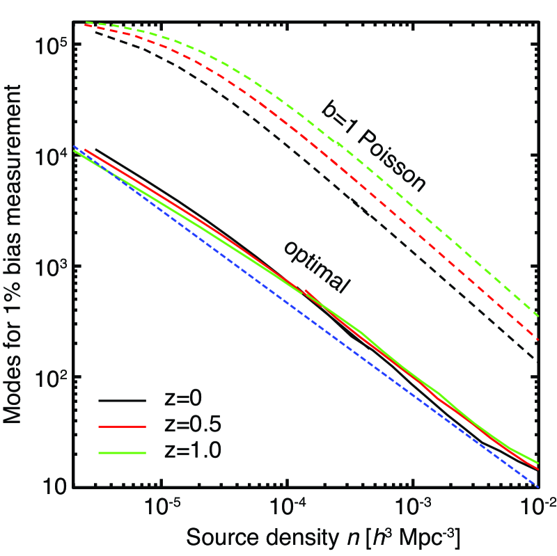
Given the high source density required to saturate the accuracy in $b$, we ask whether it is more efficient to conduct a deep survey or a shallower survey covering more sky and hence more modes. Figure 8 plots the number of modes that must be observed to determine $b$ to 1% accuracy, vs the space density $n$ of halos surveyed, as we lower $M_{\rm min}$ of the survey. We find $N_{m}\propto n^{-5/6}$ describes the results well. The total number of redshifts to be obtained in the survey is $nN_{m}\propto n^{1/6}$, hence this measure of the survey’s expense depends very weakly on depth. We also note that the source density required for the bias measurement is nearly independent of redshift using the optimal survey strategy. In contrast, a survey of number-weighted emission-line galaxies, plotted with the dashed lines, requires $>15\times$ higher $n$ than the optimal strategy at $z=0$, and galaxy densities that increase to $z=1$.

4.3 Galaxies as weights

Most measurements of large-scale structure to date have used galaxy densities as mass estimators. A spectroscopic survey of galaxies can be thought of as weighting halos by the number of galaxies per halo Scoccimarro et al. (2001). The halo occupancy distribution (HOD) gives the probability $p(N|M)$ of finding $N$ galaxies in a halo of mass $M$.

The use of galaxies as mass tracers will be inferior to an optimal halo-weighting scheme, in the sense of having higher stochasticity $E$ for a given number of redshifts, for three reasons:

1. Ideally only one redshift per halo is needed, so a galaxy survey is in some sense wasting spectroscopic resources if more than one galaxy is targeted per halo.

2. The mean HOD $g(M)\equiv\langle p(N|M)\rangle$ may not match the optimal halo weighting.

3. The occupancy of a given halo is an integer drawn from the HOD, which adds a source of stochasticity to the weight assignment and can propagate into increased stochasticity in the mass estimation, even if the mean HOD is a close to the optimal weight.

The first penalty is typically not large: the HOD is typically divided into the probability $f_{c}(M)$ of having a single central galaxy in the halo, plus a distribution $p(N_{s}|M)$ of the number $N_{s}$ of satellite galaxies. The latter is typically taken to be a Poisson distribution with a mean $\bar{N}_{s}(M)$. For most galaxy samples, the fraction of satellites is 10–20%, a small perturbation to the number of redshift targets.

This also implies, however, that $\approx 90\%$ of the halos detected in a survey are occupied by a single target galaxy, and hence given equal weight. We are then drawn to the second issue: does the mean HOD $g(M)$ serve as a nearly-optimal weight function? In Figures 1, we plot the mean number of blue galaxies (in cyan lines) and LRGs (in orange lines) in each halo as a function of halo mass, as determined from SDSS data.

For a simple HOD in which $f_{c}$ is a step function, the mean HOD is

$$g(M)=\begin{cases}1+\left(\frac{M}{M_{1}}\right)^{\alpha}&M\geq M_{0}\\ 0&M<M_{0}.\end{cases}$$ (66)

$M_{1}$, $\alpha$, and the cutoff $M_{0}$ are dependent upon the luminosity cut or other criteria used to define the galaxy sample. For luminosity-limited samples, typical values are $M_{1}\approx 20M_{0}$ and $\alpha\approx 1$ (Zehavi et al., 2005, 2010).

But note the similarity of this mean HOD functional form to Equations (44) and (56) for the optimal weight. The optimal weight for a catalog of halos with mass $M>M_{\rm min}$ is very well approximated by a function of the form $w(M)=1+(M/\beta M_{\rm min})^{\alpha}$, where $\alpha$ and $\beta$ depend on $M_{\rm min}$. For low $M_{\rm min}$, $\alpha\approx 1$, with $\alpha$ decreasing at higher $M_{\rm min}$. For $M_{\rm min}$ in the range $10^{11}$–$10^{13}M_{\odot}$ at $z=0$, values of $3<\beta<9$ yield the least stochasticity, with $E$ values indistinguishable from the optimal weighting.

Hence by a useful coincidence, the mean HOD for luminosity-selected galaxies bears close resemblance to an optimal halo weighting function, except that the HOD tends to have a longer flat low-mass plateau ($\beta\approx 20$) than the optimal weight ($\beta\approx 4$). H10 noted that the optimal weight function they derived is well approximated by equation (66), with $\beta\sim 3$, but they did not make the connection to galaxy HODs.

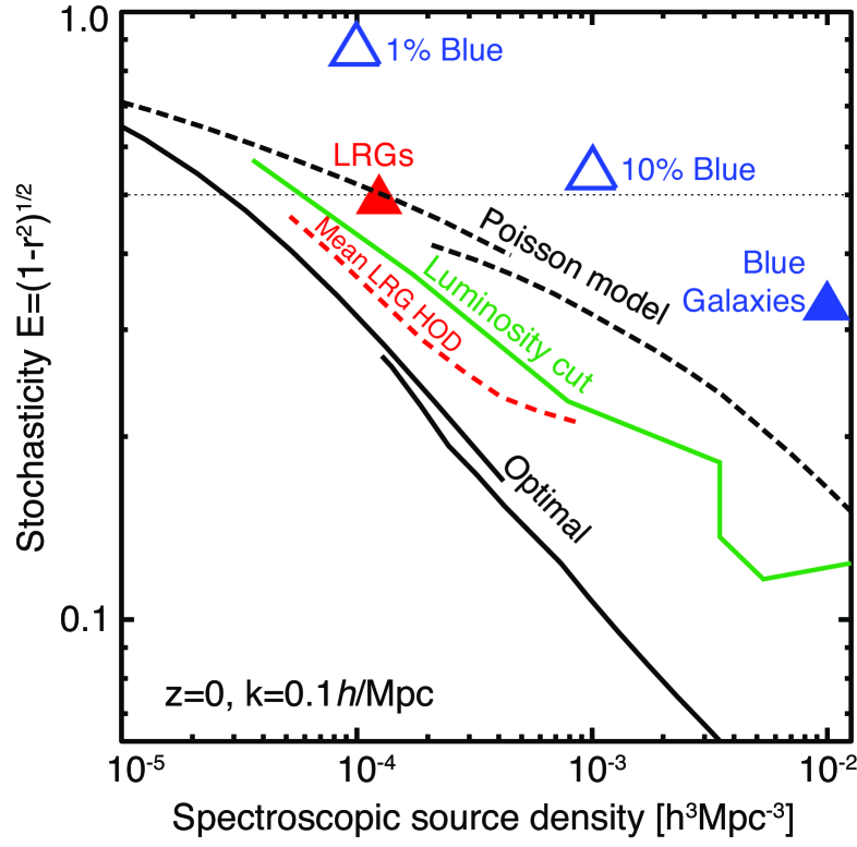
How far from optimal are the mean HODs? We examine the case of luminous red galaxies (LRGs) first. We obtain the mean number of LRGs from the HOD fitting results of Zheng et al. (2009), using equation (B3) in their paper to model the dependence of model parameter on $\sigma_{8}$. The mean HOD is shown in orange in Figure (1). Figure 9 plots the stochasticity $E$ vs the space density $n$ of target halos at $k=0.1h$Mpc^-1 and $z=0$, with the solid black line showing the best possible result from optimal targeting and weighting of halos ($M_{\rm min}$ is an implicit parameter for the black curve). The dashed red line shows the result of using the mean LRG HOD as a halo weight. A subtlety is that the LRG HOD does not have a step-function cutoff—the probability $f_{c}$ of a central galaxy follows an error function and hence has no single well-defined $M_{\rm min}$. The red dashed line shows the result of varying a low-mass cutoff applied to the LRG HOD. We find that the $E$ vs $n$ behavior is within 10–20% of the optimal result as long as we cut out halos with $f_{c}<0.1$. For LRGs, at least, the mean HOD is therefore a good choice of weight function. We will examine other galaxy classes below.

To examine the impact of item (iii), the stochasticity of the HOD, on mass-estimator performance, we populate the halos in the Millennium simulation with LRGs as per the HOD prescription. We place central galaxies in the specified fraction of halos, plus a Poisson-distributed number of satellite galaxies in the halos which host a central galaxy. The red triangle in Figure 9 shows the stochasticity $E$ vs the number density of LRGs. We find stochastically occupied halos achieve a factor of two higher (worse) $E$ than the deterministic weighting by the mean HOD. While the stochastic LRG HOD requires $\approx 3\times$ as many redshifts to reach $E=0.5$ as an ideal survey would require, it is similar to what one would predict from an optimal survey if the biased-Poisson model were a correct description of halo stochasticity (dashed black line).

The green solid curve in Figure 9 shows the result of weighting the halos by the number of galaxies drawn from HODs with varying minimum galaxy luminosities, from Zehavi et al. (2010). The behavior is similar to the LRG HOD: even though the mean number of galaxies per halo looks like the optimal weight, using the actual number of galaxies as weight results in larger $E$. The randomness in the number of galaxies in each halo introduces additional stochasticity that degrades the mass estimator.

If galaxies are to be used to provide optimal reconstructions of the mass, then they must themselves be weighted in some way so as to reduce the stochasticity in the weight applied to halos of a given mass. Determining the optimal mark is an interesting problem for the future. Formalism for treating this more general problem has been developed in Sheth (2005), and can be used directly, but is beyond the scope of this work.

Our results suggest that it is interesting to study how best to supplement the spectroscopic galaxies with a larger, deeper photometric-redshift sample. The spectroscopic galaxies can be weighted by the number of photo-z galaxies consistent with sharing the same halo. The deeper photo-z catalog potentially has lower stochasticity in halo mass estimates.

Figure 9: Stochasticity $E$ as a function of the number density of redshifts obtained in the survey.. The black lines plot the result of an ideal mass-reconstruction strategy, in which one redshift is obtained for each halo above a cutoff mass, and an optimal $w(M)$ is applied to each surveyed halo. The dotted black curve plots the stochasticity one would expect from this strategy if halos were a biased Poisson sampling of the mass—the optimal survey requires significantly fewer redshifts than predicted by the Poisson model for the same $E$. The green line gives $E$ resulting from weighting each halo by the number of galaxies above a luminosity cut—assuming galaxies occupy halos as per Zehavi et al. (2010). The blue and red triangles result from galaxy-weighting using the HODs for blue and luminous red galaxies, respectively, in the SDSS. The LRG and luminosity-cut surveys are worse than optimal primarily because of randomness in the halo occupancy; the dashed red line shows the result of eliminating this randomness by weighting each halo with the mean HOD. Blue galaxies are very inefficient for reconstructing the mass; if emission-line spectroscopic galaxies are a random 10% or 1% subsample of the blue population, they are also inefficient, not even attaining the $E=0.5$ required for a volume-limited power spectrum measurement.

Figure 10: We plot the stochasticity of an optimal mass estimator created from a catalog of halos in the Millennium simulation in the mass range $10^{12}h^{-1}M_{\odot}<M<M_{\rm max}$ vs the upper limit $M_{\rm max}$ of the halo catalog. This demonstrates that one cannot improve the stochasticity of the estimator below some floor unless one detects (and heavily weights) the rare halos above $\approx 10^{14}h^{-1}M_{\odot}$.

4.3.1 Surveys with blue or emission-line galaxies

We have seen that the mean HODs for LRGs and luminosity-selected galaxies are good approximations to the optimal weight, but the stochasticity in halo occupation degrades $E$ for a given source density $n$. Galaxy redshift surveys based on emission line detection will likely result in substantially different halo weightings, so we investigate the mass-reconstruction performance of such a survey relative to an LRG survey or optimal weighting.

We model the emission-line sample by starting with the mean HOD for blue galaxies given by equations (10) and (11) and Table 4 in (Zehavi et al., 2005):

$$g_{blue}(m)=\left(\frac{m}{M_{B}}\right)^{0.8}+0.7\,{\rm e}^{-[2\log(M/10^{12}h^{-1}M_{\odot})]^{2}}$$ (67)

where $M_{B}=7\times 10^{13}h^{-1}M_{\odot}$ and $\alpha_{B}=0.8$ (following Sheth & Diaferio, 2001). This is plotted as the cyan line in Figure 1. There is a bump in the number of blue galaxies between $\sim M^{11}~{}h^{-1}M_{\odot}$ to $\sim M^{12}~{}h^{-1}M_{\odot}$, which is very different from the optimal weight. The outcome of $E$ from weighting halos in the Millennium simulation according to galaxy counts drawn from this HOD is shown in the blue triangle of Figure (9). Although the blue galaxy sample achieves lower $E$ than the LRG does, notice that it requires $100\times$ more redshifts, i.e., is $100\times$ more costly than an optimally weighted sample. If we were to under-sample the blue galaxies—e.g. by obtaining redshifts for ten percent, or one percent of the sample with the brightest emission lines—then $E$ would rise to 0.54 and 0.86, respectively, if the sub-sampling rate is independent of halo properties. Clearly, emission line samples are a very inefficient way to reconstruct the mass, although this disadvantage is countered by the fact that emission lines can be much stronger and easily detected relative to LRG absorption features. Optimization of a survey would need to weigh these effects.

4.3.2 Surveys that under-weight massive clusters

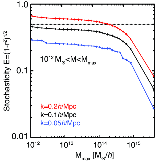
Galaxies in massive clusters tend to be strongly deficient in 21-cm emission and other gas-phase emission lines. A redshift survey selected by such criteria will tend to miss or under-weight the most massive clusters. In the Figure 10, we show that the absence of high-mass halos from a catalog sets a floor on the attainable stochasticity even with optimal mass estimation. When halos with $\sim 10^{12}h^{-1}M_{\odot}<M<M_{\rm max}$ are detected by the survey, we find that $E\approx 0.5$ is achievable at $z=0$, $k=0.2h$Mpc^-1 without detecting massive halos. However, cosmological inferences requiring lower values of $E$ require a means of detecting and appropriately weighting clusters above $10^{14}h^{-1}M_{\odot}$. Surveys without the ability to identify massive clusters reach a limit in $E$ that cannot be improved by addition of more low-mass halo detections.

The floor on $E$ can be estimated using equation (47). Consider the case when our halo catalog only contains objects below some $m_{d}$, so the “dust” is the mass in massive objects. Then $\sum_{j}n_{j}v_{j}^{2}$ can be large, so $E_{\rm pois}\to 0$. ${\cal N}_{m}$ is dominated by the most massive objects: at $z=0$, about 90% of ${\cal N}_{m}$ is contributed by objects with masses above $10^{14}h^{-1}M_{\odot}$ (we have assumed $\sigma_{8}=0.9$). If these are missing from the catalog, then ${\cal N}_{d}\to{\cal N}_{m}$, making $E_{\rm opt}\approx(1+P/{\cal N}_{m})^{-1/2}$; as a result, on scales of $k\sim 0.1h$Mpc^-1, $E_{\rm opt}$ cannot be made smaller than about 0.25.

5 Conclusion and Discussion

We have determined the weighting scheme that minimizes the stochasticity between the linearly weighted halo field and the associated mass density field. The optimal weight function depends on the mass range of the halo catalog, how much mass is missing from the halo catalogue, and how the halos cluster. (I.e., we showed how the weight is modified by a halo-mass dependent selection function.) We show that neither mass weighting nor bias weighting of the halos is optimal. The first principal component of the halo covariance matrix C is also usually not the optimal, although H10 show that the weakest PC of the altered noise matrix $\mbox{\bf C}-\mbox{\boldmath$b$}P\mbox{\boldmath$b$}^{T}$ is a good approximation to an optimal weight when the numbers of halos in all bins are equal. Rather, we demonstrate that, under very general circumstances, the optimal weight will be a mix of bias weighting and mass weighting, simply because the mass is comprised of the mass-weighted halo catalog plus the mass in the “dust bin” of structures below the halo detection threshold.

The halo model can generally give a reasonably good description for the optimal weight function and its associated stochasticity with two important alterations: first, it is necessary to treat the halos as though they sample a continuous “halo field” that is distinct from the mass distribution, and that they have a bias $v(M)$ with respect to the halo field that differs from the bias $b(M)$ with respect to mass. Second, halo catalogs extending below $10^{12}h^{-1}M_{\odot}$ do not reconstruct the mass as well as the halo model predicts. However, we find that the model generally overestimates the optimal stochasticity, even on the large scales where one might have expected to find good agreement. We suspect this is due to the combined effects of non-linear bias and halo exclusion, which our treatment currently ignores.

We also note that the randomness in the halo shapes at fixed mass—i.e. ellipticity, concentration, and/or substructure—introduces stochasticity into a mass estimator built from a halo catalog in which the halo profiles are reduced to points, setting a lower limit on the attainable $E$. In the Millennium catalog, this structure stochasticity substantially degrades the mass estimation for $k>0.2h\,{\rm Mpc}^{-1}$. Since information about halo shapes is difficult to obtain in observations, the lower limit on $E$ from point-like halos in simulations is also the best one can achieve in real observations – although, because galaxies are expected to be reasonably faithful tracers of halo profiles, it may be that they can be used to further reduce $E$ into the non-linear regime.

An optimally weighted halo catalog can have an effective number density $(nb^{2})_{\rm eff}$ up to $15\times$ better (higher) than one would have predicted for the same halo catalog in a biased-Poisson model of halo stochasticity. This gain means that a volume-limited measurement of the linear-regime power spectrum of matter for the entire observable $z<1$ universe could in principal be accomplished with only 6 million spectroscopic redshift measurements. Such a program would require outside information, perhaps a deep imaging photo-z survey, to identify halos and provide reliable mass estimates or marks to apply to spectroscopic targets. (See H10 for an estimate of the effect of mass-estimator degradation due to a generic log-normal error distribution in the estimation of halo masses.)

We use halo occupancy distribution models to estimate the stochasticity $E$ resulting from more traditional surveys which apply uniform weights to targeted galaxies. The mean HODs for luminosity-thresholded samples and LRGs are remarkably useful approximations to the optimal weight functions. However, additional stochasticity is introduced into the mass estimator by the random variations in halo occupancy about the mean. Hence luminosity-selected or LRG catalogs require $\approx 3\times$ more redshifts to reach a given $E$ than a survey with perfect knowledge of halo masses for which the optimal weighting can be applied. In contrast, HODs for blue or emission-line galaxies do not resemble the optimal weights, and hence require $\approx 100\times$ more redshift measurements than an optimally-weighted survey to obtain a given $E$. Random sub-sampling such galaxies to the same space density as LRGs yields $E$ values that are $2\times$ larger than those for LRGs. We also find that low-mass halos cannot reconstruct the shot noise contributed by the massive halos, setting an upper limit on the fidelity of the mass reconstruction for surveys that fail to identify the most massive clusters.

Application of optimal halo weighting can be even more beneficial for studies of cross-correlation between gravitational potential (i.e. mass) and other cosmological signals, since these experiments gain rapidly as the stochasticity $E$ drops below the $E=0.5$ needed to make volume-limited power-spectrum measurements. Park et al. (2010), find, for example, that mass weighting halos can greatly accuracy in estimation of gravitational potential if the halo catalog extends down to $\approx 10^{13}h^{-1}M_{\odot}$ or lower.

Applying the optimal weight is obviously efficient in reducing noise in the estimation of BAO from power spectra and in cross-correlation cosmological tests. In future work we will extend this study to the use of redshift space distortions to measure the growth rate of structure (e.g. Okumura & Jing, 2010). We are also investigating the potential for galaxy marking and non-linear mass estimators to further improve the ability to trace large-scale structure with observational data.

References

- Abbas & Sheth (2007) Abbas U., Sheth R. K., 2007, MNRAS, 378, 641
- Bardeen et al. (1986) Bardeen J. M., Bond J. R., Kaiser N., Szalay A. S., 1986, ApJ, 304, 15
- Bernstein & Jain (2004) Bernstein G., Jain B., 2004, ApJ, 600, 17
- Bonoli & Pen (2009) Bonoli S., Pen U. L., 2009, MNRAS, 396, 1610
- Cole & Kaiser (1989) Cole S., Kaiser N., 1989, MNRAS, 237, 1127
- Davis et al. (1985) Davis M., Efstathiou G., Frenk C. S., White S. D. M., 1985, ApJ, 292, 371
- Dekel & Lahav (1999) Dekel A., Lahav O., 1999, ApJ, 520, 24
- Gladders & Yee (2000) Gladders M. D., Yee H. K. C., 2000, AJ, 120, 2148
- Hamaus et al. (2010) Hamaus N., Seljak U., Desjacques V., Smith R. E., Baldauf T., 2010, ArXiv e-prints
- Hockney & Eastwood (1981) Hockney R. W., Eastwood J. W., 1981, Computer Simulation Using Particles
- Koester et al. (2007) Koester B. P., McKay T. A., Annis J., Wechsler R. H., Evrard A. E., Rozo E., Bleem L., Sheldon E. S., Johnston D., 2007, ApJ, 660, 221
- Manera et al. (2010) Manera M., Sheth R. K., Scoccimarro R., 2010, MNRAS, 402, 589
- Mo & White (1996) Mo H. J., White S. D. M., 1996, MNRAS, 282, 347
- Okumura & Jing (2010) Okumura T., Jing Y. P., 2010, ArXiv e-prints
- Park & Choi (2009) Park C., Choi Y., 2009, ApJ, 691, 1828
- Park et al. (2010) Park H., Kim J., Park C., 2010, ApJ, 714, 207
- Pen (2004) Pen U., 2004, MNRAS, 350, 1445
- Percival et al. (2004) Percival W. J., Verde L., Peacock J. A., 2004, MNRAS, 347, 645
- Scoccimarro (1998) Scoccimarro R., 1998, MNRAS, 299, 1097
- Scoccimarro et al. (2001) Scoccimarro R., Sheth R. K., Hui L., Jain B., 2001, ApJ, 546, 20
- Seljak et al. (2009) Seljak U., Hamaus N., Desjacques V., 2009, Physical Review Letters, 103, 091303
- Seljak & Warren (2004) Seljak U., Warren M. S., 2004, MNRAS, 355, 129
- Seljak & Zaldarriaga (1996) Seljak U., Zaldarriaga M., 1996, ApJ, 469, 437
- Sheth (2005) Sheth R. K., 2005, MNRAS, 364, 796
- Sheth et al. (2005) Sheth R. K., Connolly A. J., Skibba R., 2005, ArXiv Astrophysics e-prints
- Sheth & Diaferio (2001) Sheth R. K., Diaferio A., 2001, MNRAS, 322, 901
- Sheth & Jain (2003) Sheth R. K., Jain B., 2003, MNRAS, 345, 529
- Sheth & Lemson (1999) Sheth R. K., Lemson G., 1999, MNRAS, 304, 767
- Sheth & Tormen (1999) Sheth R. K., Tormen G., 1999, MNRAS, 308, 119
- Sheth & Tormen (2002) Sheth R. K., Tormen G., 2002, MNRAS, 329, 61
- Smith et al. (2007) Smith R. E., Scoccimarro R., Sheth R. K., 2007, Phys. Rev. D, 75, 063512
- Springel (2005) Springel V., 2005, MNRAS, 364, 1105
- Springel et al. (2005) Springel V., White S. D. M., Jenkins A., Frenk C. S., Yoshida N., Gao L., Navarro J., Thacker R., Croton D., Helly J., Peacock J. A., Cole S., Thomas P., Couchman H., Evrard A., Colberg J., Pearce F., 2005, Nature, 435, 629
- Sunyaev & Zeldovich (1972) Sunyaev R. A., Zeldovich Y. B., 1972, Comments on Astrophysics and Space Physics, 4, 173
- Tegmark et al. (1997) Tegmark M., Taylor A. N., Heavens A. F., 1997, ApJ, 480, 22
- White (1996) White S. D. M., 1996, in Schaeffer R., Silk J., Spiro M., Zinn-Justin J., eds, Cosmology and Large-Scale Structure, Elsevier, Amsterdam p. 349
- Zehavi et al. (2010) Zehavi I., Zheng Z., Weinberg D. H., Blanton M. R., Bahcall N. A., Berlind A. A., Brinkmann J., Frieman J. A. e. a., 2010, ArXiv e-prints
- Zehavi et al. (2005) Zehavi I., Zheng Z., Weinberg D. H., Frieman J. A., Berlind A. A., Blanton M. R., Scoccimarro R., Sheth R. K. e. a., 2005, ApJ, 630, 1
- Zheng et al. (2009) Zheng Z., Zehavi I., Eisenstein D. J., Weinberg D. H., Jing Y. P., 2009, ApJ, 707, 554