Approximate Nearest Neighbor Search for Low Dimensional Queries

Abstract

We study the Approximate Nearest Neighbor problem for metric spaces where the query points are constrained to lie on a subspace of low doubling dimension, while the data is high-dimensional. We show that this problem can be solved efficiently despite the high dimensionality of the data.

1 Introduction

The nearest neighbor problem is the following. Given a set $\mathsf{P}$ of $n$ data points in a metric space $\mathcal{X}$, preprocess $\mathsf{P}$, such that given a query point $\mathtt{q}\in\mathcal{X}$, one can find (quickly) the point $\mathsf{n}_{\mathtt{q}}\in\mathsf{P}$ closest to $\mathtt{q}$. Nearest neighbor search is a fundamental task used in numerous domains including machine learning, clustering, document retrieval, databases, statistics, and many others.

Exact nearest neighbor.

The (exact) nearest neighbor problem has a naive linear time algorithm without any preprocessing. However, by doing some nontrivial preprocessing, one can achieve a sublinear search time for the nearest neighbor. In $d$-dimensional Euclidean space (i.e., ${\rm I\!R}^{d}$) this is facilitated by answering point location queries using a Voronoi diagram [dBCvKO08]. However, this approach is only suitable for low dimensions, as the complexity of the Voronoi diagram is $\Theta\left({n^{\left\lceil{d/2}\right\rceil}}\right)$ in the worst case. Specifically, Clarkson [Cla88] showed a data-structure with query time $O\!\left({{\log n}}\right)$ time, and $O\!\left({{n^{\left\lceil{d/2}\right\rceil+\delta}}}\right)$ space, where $\delta>0$ is a prespecified constant (the $O(\cdot)$ notation here hides constants that are exponential in the dimension). One can tradeoff the space used and the query time [AM93]. Meiser [Mei93] provided a data-structure with query time $O\!\left({{d^{5}\log n}}\right)$, which has polynomial dependency on the dimension, where the space used is $O\!\left({{n^{d+\delta}}}\right)$. These solutions are impractical even for data-sets of moderate size if the dimension is larger than two.

Approximate nearest neighbor.

In typical applications, it is usually sufficient to return an approximate nearest neighbor (ANN). Given an ${\varepsilon}>0$, a $(1+{\varepsilon})$-ANN to a query point $\mathtt{q}$, is a point $y\in\mathsf{P}$, such that

$$\mathsf{d}\!\left({{\mathtt{q}},{y}}\right)\leq(1+{\varepsilon})\mathsf{d}\!\left({{\mathtt{q}},{\mathsf{n}_{\mathtt{q}}}}\right),$$

where $\mathsf{n}_{\mathtt{q}}\in\mathsf{P}$ is the nearest neighbor to $\mathtt{q}$ in $\mathsf{P}$. Considerable amount of work was done on this problem, see [Cla06] and references therein.

In high dimensional Euclidean space, Indyk and Motwani showed that ANN can be reduced to a small number of near neighbor queries [IM98, HIM12]. Next, using locality sensitive hashing they provide a data-structure that answers ANN queries in time (roughly) $\widetilde{O}\!\left({n^{1/(1+{\varepsilon})}}\right)$ and preprocessing time and space $\widetilde{O}\!\left({n^{1+1/(1+{\varepsilon})}}\right)$; here the $\widetilde{O}\!\left({\cdot}\right)$ hides terms polynomial in $\log n$ and $1/{\varepsilon}$. This was improved to $\widetilde{O}\!\left({n^{1/(1+{\varepsilon})^{2}}}\right)$ query time, and preprocessing time and space $\widetilde{O}\!\left({n^{1+1/(1+{\varepsilon})^{2}}}\right)$ [AI06, AI08]. These bounds are near optimal [MNP06, OWZ11].

In low dimensions (i.e., ${\rm I\!R}^{d}$), one can use linear space (independent of ${\varepsilon}$) and get ANN query time $O(\log n+1/{\varepsilon}^{d-1})$ [AMN⁺98, Har11]. Interestingly, for this data-structure, the approximation parameter ${\varepsilon}$ is not prespecified during the construction; one needs to provide it only during the query. An alternative approach is to use Approximate Voronoi Diagrams (AVD), introduced by Har-Peled [Har01], which are partition of space into regions, desirably of low complexity, typically with a representative point for each region that is an ANN for any point in the region. In particular, Har-Peled showed that there is such a decomposition of size $O\!\left({(n/{\varepsilon}^{d})\log^{2}n}\right)$, such that ANN queries can be answered in $O(\log(n/{\varepsilon}))$ time. Arya and Malamatos [AM02] showed how to build AVDs of linear complexity (i.e., $O(n/{\varepsilon}^{d})$). Their construction uses Well Separated Pair Decompositions [CK95]. Further tradeoffs between query and space for AVDs were studied by Arya et al. [AMM09].

Metric spaces.

One possible approach for the more general case when the data lies in some abstract metric space, is to define a notion of dimension and develop efficient algorithms in these settings. This approach is motivated by the belief that real world data is “low dimensional” in many cases, and should be easier to handle than true high dimensional data. An example of this approach is the notion of doubling dimension [Ass83, Hei01, GKL03]. The doubling constant of metric space $\mathcal{X}$ is the maximum, over all balls $\mathsf{b}$ in the metric space $\mathcal{X}$, of the minimum number of balls needed to cover $\mathsf{b}$, using balls with half the radius of $\mathsf{b}$. The logarithm of the doubling constant is the doubling dimension of the space. The doubling dimension can be thought of as a generalization of the Euclidean dimension, as ${\rm I\!R}^{d}$ has doubling dimension $\Theta(d)$. Furthermore, the doubling dimension extends the notion of growth restricted metrics of Karger and Ruhl [KR02].

The problem of ANN in spaces of low doubling dimension was studied before, see [KR02, HKMR04]. Talwar [Tal04] presented several algorithms for spaces of low doubling dimension. Some of them were however dependent on the spread of the point set. Krauthgamer and Lee [KL04] presented a net navigation algorithm for ANN in spaces of low doubling dimension. Har-Peled and Mendel [HM06] provided data-structures for ANN search that use linear space and match the bounds known for ${\rm I\!R}^{d}$ [AMN⁺98]. Clarkson [Cla06] presents several algorithms for nearest neighbor search in low dimensional spaces for various notions of dimensions.

ANN in high and low dimensions.

As indicated above, the ANN problem is easy in low dimensions (either Euclidean or bounded doubling dimension). If the dimension is high the problem is considerably more challenging. There is considerable work on ANN in high dimensional Euclidean space (see [IM98, KOR00, HIM12]) but the query time is only slightly sublinear if ${\varepsilon}$ is close to $0$. In general metric spaces, it is easy to argue that (in the worst case) the ANN algorithm must compute the distance of the query point to all the input points.

It is natural to ask therefore what happens when the data (or the queries) come from a low dimensional subspace that lies inside a high dimensional ambient space. Such cases are interesting as it is widely believed that in practice real world data usually lies on a low dimensional manifold (or is close to lying on such a manifold). Such low-dimensionality arises from the way the data is being acquired, inherent dependency between parameters, aggregation of data that leads to concentration of mass phenomena, etc.

Indyk and Naor [IN07] showed that if the data is in high dimensional Euclidean space, but lies on a manifold with low doubling dimension, then one can do a dimension reduction into constant dimension (i.e., similar in spirit to the JL lemma [JL84]), such that $(1+{\varepsilon})$-ANN to a query point (the query point might lie anywhere in the ambient space) is preserved with constant probability. Using an appropriate data-structure on the embedded space and repeating this process sufficient number of times results in a data-structure that can answer such ANN queries in polylog time (ignoring the dependency on ${\varepsilon}$).

The problem.

In this paper, we study the “reverse” problem. Here we are given a high dimensional data set $\mathsf{P}$, and we would like to preprocess it for ANN queries, where the queries come from a low-dimensional subspace/manifold $\mathcal{M}$. The question arises naturally when the given data is formed by merging together a large number of data sets, while the ANN queries come from a single data set.

In particular, the conceptual question here is whether this problem is low or high dimensional in nature. Note that direct dimension reduction as done by Indyk and Naor would not work in this case. Indeed, imagine the data lies densely on a slightly deformed sphere in high dimensions, and the query is the center of the sphere. Clearly, a random dimension reduction via projection into constant dimension would not preserve the $(1+{\varepsilon})$-ANN.

Our results.

Given a point set $\mathsf{P}$ lying in a general metric space $\mathcal{X}$ (which is not necessarily Euclidean and is conceptually high dimensional), and a subspace $\mathcal{M}$ having low doubling dimension $\tau$, we show how to preprocess $\mathsf{P}$ such that given any query point in $\mathcal{M}$ we can quickly answer $(1+{\varepsilon})$-ANN queries on $\mathsf{P}$. In particular, we get data-structures of (roughly) linear size that answer $(1+{\varepsilon})$-ANN queries in (roughly) logarithmic time.

Our construction uses ideas developed for handling the low dimensional case. Initially, we embed $\mathsf{P}$ and $\mathcal{M}$ into a space with low doubling dimension that (roughly) preserves distances between $\mathcal{M}$ and $\mathsf{P}$. We can use the embedded space to answer constant factor ANN queries. Getting a better approximation requires some further ideas. In particular, we build a data-structure over $\mathcal{M}$ that is somewhat similar to approximate Voronoi diagrams [Har01]. By sprinkling points carefully on the subspace $\mathcal{M}$ and using the net-tree data-structure [HM06] we can answer $(1+{\varepsilon})$-ANN queries in time $O({\varepsilon}^{-O(\tau)}+2^{O(\tau)}\log n)$.

To get a better query time requires some further work. In particular, we borrow ideas from the simplified construction of Arya and Malamatos [AM02] (see also [AMM09]). Naively, this requires us to use well separated pairs decomposition (i.e., WSPD) [CK95] for $\mathsf{P}$. Unfortunately, no such small WSPD exists for data in high dimensions. To overcome this problem, we build the WSPD in the embedded space. Next, we use this to guide us in the construction of the ANN data-structure. This results in a data-structure that can answer $(1+{\varepsilon})$-ANN queries in $O(2^{O(\tau)}\log n)$ time. See Section 5 for details.

We also present an algorithm for a weaker model, where the query subspace is not given to us directly. Instead, every time an ANN query is issued, the algorithm computes a region around the query point such that the returned point is a valid ANN for all the points in this region. Furthermore, the algorithm caches such regions, and whenever a query arrives it first checks if the query point is already contained in one of the regions computed, and if so it answers the ANN query immediately. Significantly, for this algorithm we need no prespecified knowledge about the query subspace. The resulting algorithm computes on the fly AVD on the query subspace. In particular, we show that if the queries come from a subspace with doubling dimension $\tau$, then the algorithm would create at most $n/{\varepsilon}^{O\left({{\tau}}\right)}$ regions overall. A limitation of this new algorithm is that we do not currently know how to efficiently perform a point-location query in a set of such regions, without assuming further knowledge about the subspace. Interestingly, the new algorithm can be interpreted as learning the underlying subspace/manifold the queries come from. See Section 6 for the precise result.

Organization.

In Section 2, we define some basic concepts, and as a warm-up exercise study the problem where the subspace $\mathcal{M}$ is a linear subspace of ${\rm I\!R}^{d}$ – this provides us with some intuition for the general case. We also present the embedding of $\mathsf{P}$ and $\mathcal{M}$ into the subspace $\mathcal{M}^{\prime}$, which has low doubling dimension while (roughly) preserving distances of interest. In Section 3, we provide a data-structure for constant factor ANN using this embedding. In Section 4, we use the constant ANN to get a data-structure for answering $(1+{\varepsilon})$-ANN. In Section 5, we use WSPD to build a data-structure that is similar in spirit to AVDs. This results in a data-structure with slightly faster ANN query time. The on the fly construction of AVD to answer ANN queries without assuming any knowledge of the query subspace is described in Section 6. Finally, conclusions are provided in Section 7.

2 Preliminaries

2.1 Problem and Model

The Problem.

We look at the ANN problem in the following setting. Given a set $\mathsf{P}$ of $n$ data points in a metric space $\mathcal{X}$, and a set $\mathcal{M}\subseteq\mathcal{X}$ of (hopefully low) doubling dimension $\tau$, and ${\varepsilon}>0$, we want to preprocess the points of $\mathsf{P}$, such that given a query point $\mathtt{q}\in\mathcal{M}$ one can efficiently find a $(1+{\varepsilon})$-ANN of $\mathtt{q}$ in $\mathsf{P}$.

Model.

We are given a metric space $\mathcal{X}$ and a subset $\mathcal{M}\subseteq\mathcal{X}$ of doubling dimension $\tau$. We assume that the distance between any pair of points can be computed in constant time in a black-box fashion. Specifically, for any $\mathsf{p},q\in\mathcal{X}$ we denote by $\mathsf{d}\!\left({{\mathsf{p}},{q}}\right)$ the distance between $\mathsf{p}$ and $q$. We also assume that one can build nets on $\mathcal{M}$. Specifically, given a point $\mathsf{p}\in\mathcal{M}$ and a radius $r>0$, we assume we can compute $2^{\tau}$ points $\mathsf{p}_{i}\in\mathcal{M}$, such that $\mathsf{ball}\!\left({{\mathsf{p}},{r}}\right)\cap\mathcal{M}\subseteq\bigcup\mathsf{ball}\!\left({{\mathsf{p}_{i}},{r/2}}\right)$. By applying this recursively we can compute an $r$-net $N$ for any $\mathsf{ball}\!\left({{\mathsf{p}},{R}}\right)$ centered at $\mathsf{p}$; that is, for any point $v\in\mathsf{ball}\!\left({{\mathsf{p}},{R}}\right)$ there exists a point $u\in N$ such that $\mathsf{d}\!\left({{v},{u}}\right)\leq r$. Let compNet$(\mathsf{p},R,r)$ denote this algorithm for computing this $r$-net. The size of $N$ is $(R/r)^{O(\tau)}$, and we assume this also bounds the time it takes to compute it. For example, in Euclidean space ${\rm I\!R}^{d}$, let $\mathsf{p}$ be the origin and consider the tiling of space by a grid of cubes of diameter $r$. One can compute an $r$-net, by simply enumerating all the vertices of the grid cells that intersect the cube $\left[{-R,R}\rule[0.0pt]{0.0pt}{8.5359pt}\right]^{d}$ surrounding $\mathsf{ball}\!\left({{\mathsf{p}},{R}}\right)=\mathsf{ball}\!\left({{0},{R}}\right)$.

Finally, given any point $\mathsf{p}\in\mathcal{X}$ we assume that one can compute, in $O\!\left({{1}}\right)$ time, a point $\alpha({\mathsf{p}})\in\mathcal{M}$ such that $\alpha({\mathsf{p}})$ is the closest point in $\mathcal{M}$ to $\mathsf{p}$. (Alternatively, $\alpha({\mathsf{p}})$ might be specified for each point of $\mathsf{P}$ in advance.)

Spread of a point set.

For a point set $\mathsf{P}$, the spread is the ratio $\frac{\max\limits_{\mathsf{p},v\in\mathsf{P}}\mathsf{d}\left({{\mathsf{p}},{v}}\right)}{\min\limits_{\mathsf{p},v\in\mathsf{P},\mathsf{p}\neq v}\mathsf{d}\left({{\mathsf{p}},{v}}\right)}$. The following result is elementary.

Lemma 2.1.

Let $\mathcal{M}$ be a metric space of doubling dimension $\tau$ and $\mathsf{P}\subseteq\mathcal{M}$ be a point set with spread $\lambda$. Then $\left\lvert{\mathsf{P}}\right\rvert\leq\lambda^{O\left({{\tau}}\right)}$.

Well separated pairs decomposition.

For a point set $\mathsf{P}$, a pair decomposition of $\mathsf{P}$ is a set of pairs $\mathcal{W}=\left\{{\rule[-5.69046pt]{0.0pt}{11.38092pt}\left\{{A_{1},B_{1}}\right\},\ldots,\left\{{A_{s},B_{s}}\right\}}\right\}$, such that (I) $A_{i},B_{i}\subset\mathsf{P}$for every $i$, (II) $A_{i}\cap B_{i}=\emptyset$for every $i$, and (III) $\cup_{i=1}^{s}A_{i}\otimes B_{i}=\mathsf{P}\otimes\mathsf{P}$. Here $X\otimes Y=\left\{{\rule[-5.69046pt]{0.0pt}{11.38092pt}\left\{{x,y}\right\}\,\left|\,{x}\rule[-5.69046pt]{0.0pt}{11.38092pt}\right.\in X,y\in Y,\text{ and }x\neq y}\right\}$.

A pair $\mathsf{Q}\subseteq\mathsf{P}$ and $\mathsf{R}\subseteq\mathsf{P}$ is $(1/{\varepsilon})$-separated if $\max\!\left({\mathrm{d{}i{}am}\!\left({\mathsf{Q}}\right),\mathrm{d{}i{}am}\!\left({\mathsf{R}}\right)}\right)\leq{\varepsilon}\cdot\mathsf{d}\!\left({{\mathsf{Q}},{\mathsf{R}}}\right)$, where $\mathsf{d}\!\left({{\mathsf{Q}},{\mathsf{R}}}\right)=\min_{\mathsf{p}\in\mathsf{Q},v\in\mathsf{R}}\mathsf{d}\!\left({{\mathsf{p}},{v}}\right)$. For a point set $\mathsf{P}$, a well-separated pair decomposition (WSPD) of $\mathsf{P}$ with parameter $1/{\varepsilon}$ is a pair decomposition of $\mathsf{P}$ with a set of pairs $\mathcal{W}=\left\{{\left\{{A_{1},B_{1}}\right\},\ldots,\left\{{A_{s},B_{s}}\right\}}\right\}$, such that, for any $i$, the sets $A_{i}$ and $B_{i}$ are ${\varepsilon}^{-1}$-separated [CK95].

2.1.1 Net-trees

The net-tree [HM06] is a data-structure that defines hierarchical nets in finite metric spaces. Formally, a net-tree is defined as follows: Let $\mathsf{P}\subseteq\mathcal{M}$ be a finite subset. A net-tree of $\mathsf{P}$ is a tree $T$ whose set of leaves is $\mathsf{P}$. Denote by $\mathsf{P}_{v}$ the set of leaves in the subtree rooted at a vertex $v\in T$. With each vertex $v$ is associated a point $\mathrm{rep}_{v}\in\mathsf{P}_{v}$. Internal vertices have at least two children. Each vertex $v$ has a level $l\!\left({v}\right)\in\mathbb{Z}\cup\left\{{-\infty}\right\}$. The levels satisfy $l\!\left({v}\right)<l\!\left({\overline{p}\!\left({v}\right)}\right)$, where $\overline{p}\!\left({v}\right)$ is the parent of $v$ in $T$. The levels of the leaves are $-\infty$. Let $\gamma$ be some large constant, say $\gamma=11$. The following properties are satisfied: (I) For every vertex $v\in T$, $\mathsf{ball}\!\left({{\mathrm{rep}_{v}},{\frac{2\gamma}{\gamma-1}\gamma^{l\left({v}\right)}}}\right)\supseteq\mathsf{P}_{v}$, (II) For every vertex $v\in T$ that is not the root, $\mathsf{ball}\!\left({{\mathrm{rep}_{v}},{\frac{\gamma-5}{2(\gamma-1)}\gamma^{l\left({\overline{p}\left({v}\right)}\right)-1}}}\right)\cap\mathsf{P}\subseteq\mathsf{P}_{v}$, (III) For every internal vertex $u\in T$, there exists a child $v\in T$ of $u$ such that $\mathrm{rep}_{u}=\mathrm{rep}_{v}$.

2.2 Warm-up exercise: Affine Subspace

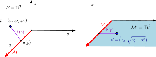
Figure 1: An example of embedding of space into two dimensions where $\mathcal{M}$ is the $x$-axis.

We first consider the case where our query subspace is an affine subspace embedded in $d$ dimensional Euclidean space. Thus let $\mathcal{X}={\rm I\!R}^{d}$ with the usual Euclidean metric. Suppose our query subspace $\mathcal{M}$ is an affine subspace of dimension $k$ where $k\ll d$. We are also given $n$ data points $\mathsf{P}=\left\{{\mathsf{p}_{1},\mathsf{p}_{2},\ldots,\mathsf{p}_{n}}\right\}$. We want to preprocess $\mathsf{P}$ such that given a $\mathtt{q}\in\mathcal{M}$ we can quickly find a point $\mathsf{p}_{i}\in\mathsf{P}$ which is a $(1+{\varepsilon})$-ANN of $\mathtt{q}$ in $\mathsf{P}$.

We choose an orthonormal system of coordinates for $\mathcal{M}$. Denote the projection of a point $\mathsf{p}$ to $\mathcal{M}$ as $\alpha({\mathsf{p}})$. Denote the coordinates of a point $\alpha({\mathsf{p}})\in\mathcal{M}$ in the chosen coordinate system as $(\mathsf{p}^{1},\mathsf{p}^{2},\dots,\mathsf{p}^{k})$. Let $0pt{\mathsf{p}}$ denote the distance of any $\mathsf{p}\in{\rm I\!R}^{d}$ from the subspace $\mathcal{M}$. Notice that $0pt{\mathsf{p}}=\left\|{\mathsf{p}}-{\alpha({\mathsf{p}})}\right\|$, and consider the following embedding.

Definition 2.2.

For the point $\mathsf{p}\in{\rm I\!R}^{d}$, the embedded point is $\mathsf{p}^{\prime}=\left({\rule[0.0pt]{0.0pt}{9.95863pt}\mathsf{p}^{1},\mathsf{p}^{2},\dots,\mathsf{p}^{k},0pt{\mathsf{p}}}\right)\in{\rm I\!R}^{k+1}$.

An example of the above embedding is shown in Figure 1. It is easy to see that for $x\in\mathcal{M}$ and $y\in{\rm I\!R}^{d}$, by the Pythagorean theorem, we have $\left\|{x}-{y}\right\|^{2}=\left\|{x}-{\alpha({y})}\right\|^{2}+\left\|{\alpha({y})}-{y}\right\|^{2}=\left\|{x}-{\alpha({y})}\right\|^{2}+0pt{y}^{2}=\left\|{x^{\prime}}-{y^{\prime}}\right\|^{2}$. So, $\left\|{x}-{y}\right\|=\left\|{x^{\prime}}-{y^{\prime}}\right\|$. That is, the above embedding preserves the distances between points on $\mathcal{M}$ and any point in ${\rm I\!R}^{d}$.

As such, given a query point $\mathtt{q}\in\mathcal{M}$, let $\mathsf{p}_{i}^{\prime}$ be its $(1+{\varepsilon})$-ANN in $\mathsf{P}^{\prime}\subseteq{\rm I\!R}^{k+1}$. Then the original point $\mathsf{p}_{i}\in\mathsf{P}$ (that generated $\mathsf{p}_{i}^{\prime}$) is a $(1+{\varepsilon})$-ANN of $\mathtt{q}$ in the original space ${\rm I\!R}^{d}$.

But this is easy to do using known data-structures for ANN [AMN⁺98], or the data-structures for approximate Voronoi diagram [Har01, AM02].

Thus, we have $n$ points in ${\rm I\!R}^{k+1}$ to preprocess and, without loss of generality, we can assume that $\mathsf{p}_{i}^{\prime}$ are all distinct. Now given ${\varepsilon}\leq 1/2$, we can preprocess the points $\left\{{\mathsf{p}_{1}^{\prime},\dots,\mathsf{p}_{n}^{\prime}}\right\}$ and construct an approximate Voronoi diagram consisting of $O\!\left({{n{\varepsilon}^{-(k+1)}\log{\varepsilon}^{-1}}}\right)$ regions [AM02]. Each such region is the difference of two cubes. Given a point $\mathtt{q}^{\prime}\in{\rm I\!R}^{k+1}$ we can find a $(1+{\varepsilon})$-ANN in $O\!\left({{\log\!\left({{n}/{{\varepsilon}}}\right)}}\right)$ time, using this data-structure.

2.3 An Embedding

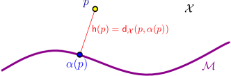
Figure 2: The quantities $\alpha({\mathsf{p}})$ and $0pt{\mathsf{p}}$.

Here, we show how to embed the points of $\mathsf{P}$ (and all of $\mathcal{X}$) into another metric space $\mathcal{M}^{\prime}$ with finite doubling dimension, such that the distances between $\mathsf{P}$ and $\mathcal{M}$ are roughly preserved.

For a point $\mathsf{p}\in\mathcal{X}$, let $\alpha({\mathsf{p}})$ denote the closest point in $\mathcal{M}$ to $\mathsf{p}$ (for the sake of simplicity of exposition we assume this point is unique). The height of a point $\mathsf{p}\in\mathcal{X}$ is the distance between $\mathsf{p}$ and $\alpha({\mathsf{p}})$; namely, $0pt{\mathsf{p}}=\mathsf{d}_{{\mathcal{X}}}\!\left({{\mathsf{p}},{\alpha({\mathsf{p}})}}\right)$. For a set $\mathsf{B}\subseteq\mathcal{X}$, let $\alpha({\mathsf{B}})$ denote the set $\left\{{\alpha({x})\,\left|\,{x\in\mathsf{B}}\rule[-5.69046pt]{0.0pt}{11.38092pt}\right.}\right\}$. An example is shown in Figure 2.

Definition 2.3 ($\mathcal{M}^{\prime}$ embedding.).

Consider the embedding of $\mathcal{X}$ into $\mathcal{M}^{\prime}=\mathcal{M}\times{\rm I\!R}^{+}$ induced by the distances of points of $\mathcal{X}$ from $\mathcal{M}$. Formally, for a point $\mathsf{p}\in\mathcal{X}$, the embedding is defined as

$$\mathsf{p}^{\prime}=\!\left({\rule[0.0pt]{0.0pt}{9.95863pt}\alpha({\mathsf{p}}),\,0pt{\mathsf{p}}}\right)\in\mathcal{M}^{\prime}.$$

The distance between any two points $\mathsf{p}^{\prime}=\!\left({\alpha({\mathsf{p}}),0pt{\mathsf{p}}}\right)$ and $v^{\prime}=\!\left({\alpha({v}),0pt{v}}\right)$ of $\mathcal{M}^{\prime}$ is defined as

$$\mathsf{d}_{{\mathcal{M}^{\prime}}}\!\left({{\mathsf{p}^{\prime}},{v^{\prime}}}\right)=\mathsf{d}_{{\mathcal{X}}}\!\left({{\rule[0.0pt]{0.0pt}{9.95863pt}\alpha({\mathsf{p}})},{\alpha({v})}}\right)+\left\lvert{0pt{\mathsf{p}}-0pt{v}}\right\rvert.$$

It is easy to verify that $\mathsf{d}_{{\mathcal{M}^{\prime}}}\!\left({{\cdot},{\cdot}}\right)$ complies with the triangle inequality. For the sake of simplicity of exposition, we assume that for any two distinct points $\mathsf{p}$ and $v$ in our (finite) input point set $\mathsf{P}$ it holds that $\mathsf{p}^{\prime}\neq v^{\prime}$ (that is, $\mathsf{d}_{{\mathcal{M}^{\prime}}}\!\left({{\mathsf{p}^{\prime}},{v^{\prime}}}\right)\neq 0$). This can be easily guaranteed by introducing symbolic perturbations.

Lemma 2.4.

The following holds: (A) For any two points $x,y\in\mathcal{M}$, we have $\mathsf{d}_{{\mathcal{M}^{\prime}}}\!\left({{x^{\prime}},{y^{\prime}}}\right)=\mathsf{d}_{{\mathcal{X}}}\!\left({{x},{y}}\right)$. (B) For any point $x\in\mathcal{M}$ and $y\in\mathcal{X}$, we have $\mathsf{d}_{{\mathcal{X}}}\!\left({{x},{y}}\right)\leq\mathsf{d}_{{\mathcal{M}^{\prime}}}\!\left({{x^{\prime}},{y^{\prime}}}\right)\leq 3\mathsf{d}_{{\mathcal{X}}}\!\left({{x},{y}}\right)$. (C) The space $\mathcal{M}^{\prime}$ has doubling dimension at most $2\tau+2$, where $\tau$ is the doubling dimension of $\mathcal{M}$.

Proof.

(A) Clearly, for $x,y\in\mathcal{M}$, we have $x^{\prime}=(x,0)$ and $y^{\prime}=(y,0)$. As such, $\mathsf{d}_{{\mathcal{M}^{\prime}}}\!\left({{x^{\prime}},{y^{\prime}}}\right)=\mathsf{d}_{{\mathcal{X}}}\!\left({{x},{y}}\right)+|0-0|=\mathsf{d}_{{\mathcal{X}}}\!\left({{x},{y}}\right)$.

(B) Let $x\in\mathcal{M}$ and $y\in\mathcal{X}$. We have $x^{\prime}=(x,0)$ and $y^{\prime}=\!\left({\rule[0.0pt]{0.0pt}{9.95863pt}\alpha({y}),\mathsf{d}_{{\mathcal{X}}}\!\left({{y},{\alpha({y})\rule[0.0pt]{0.0pt}{8.5359pt}}}\right)}\right)$. As such,

$$\mathsf{d}_{{\mathcal{M}^{\prime}}}\!\left({{x^{\prime}},{y^{\prime}}}\right) =\mathsf{d}_{{\mathcal{X}}}\!\left({{\alpha({x})},{\alpha({y})}}\right)+\left\lvert{0-0pt{y}}\right\rvert=\mathsf{d}_{{\mathcal{X}}}\!\left({{x},{\alpha({y})}}\right)+\mathsf{d}_{{\mathcal{X}}}\!\left({{\alpha({y})},{y}}\right)\geq\mathsf{d}_{{\mathcal{X}}}\!\left({{x},{y}}\right),$$

by the triangle inequality. On the other hand, because $\mathsf{d}_{{\mathcal{X}}}\!\left({{y},{\alpha({y})}}\right)=\mathsf{d}_{{\mathcal{X}}}\!\left({{y},{\mathcal{M}}}\right)\leq\mathsf{d}_{{\mathcal{X}}}\!\left({{x},{y}}\right)$, we have

$$\mathsf{d}_{{\mathcal{M}^{\prime}}}\!\left({{x^{\prime}},{y^{\prime}}}\right) =\mathsf{d}_{{\mathcal{X}}}\!\left({{\rule[0.0pt]{0.0pt}{9.95863pt}\alpha({x})},{\alpha({y})}}\right)+\left\lvert{0pt{x}-0pt{y}}\right\rvert=\mathsf{d}_{{\mathcal{X}}}\!\left({{\rule[0.0pt]{0.0pt}{9.95863pt}x},{\alpha({y})}}\right)+0pt{y}$$

$$=\mathsf{d}_{{\mathcal{X}}}\!\left({{x},{\alpha({y})}}\right)+\mathsf{d}_{{\mathcal{X}}}\!\left({{y},{\alpha({y})}}\right)\leq\!\left({\rule[0.0pt]{0.0pt}{9.95863pt}\mathsf{d}_{{\mathcal{X}}}\!\left({{x},{y}}\right)+\mathsf{d}_{{\mathcal{X}}}\!\left({{y},{\alpha({y})}}\right)}\right)+\mathsf{d}_{{\mathcal{X}}}\!\left({{y},{\alpha({y})}}\right)$$

$$=\mathsf{d}_{{\mathcal{X}}}\!\left({{x},{y}}\right)+2\mathsf{d}_{{\mathcal{X}}}\!\left({{y},{\alpha({y})}}\right)\leq 3\mathsf{d}_{{\mathcal{X}}}\!\left({{x},{y}}\right),$$

by the triangle inequality.

(C) Consider a point $(\mathsf{p},\psi)\in\mathcal{M}\times{\rm I\!R}^{+}=\mathcal{M}^{\prime}$ and the ball $\mathsf{b}=\mathsf{ball}_{\mathcal{M}^{\prime}}\!\left({{(\mathsf{p},\psi)},{r}}\right)\subseteq\mathcal{M}^{\prime}$ of radius $r$ centered at $(\mathsf{p},\psi)$. Consider the projection of $\mathsf{b}$ into $\mathcal{M}$; that is $\mathsf{P}_{\mathcal{M}}=\left\{{v\,\left|\,{\!\left({v,h}\right)\in\mathsf{b}}\rule[-5.69046pt]{0.0pt}{11.38092pt}\right.}\right\}$. Similarly, let $\mathsf{P}_{{\rm I\!R}}=\left\{{h\,\left|\,{\!\left({v,h}\right)\in\mathsf{b}}\rule[-5.69046pt]{0.0pt}{11.38092pt}\right.}\right\}$.

Clearly, $\mathsf{ball}_{\mathcal{M}^{\prime}}\!\left({{\rule[0.0pt]{0.0pt}{8.5359pt}(\mathsf{p},\psi)},{r}}\right)\subseteq\mathsf{P}_{\mathcal{M}}\times\mathsf{P}_{{\rm I\!R}}$, and $\mathsf{P}_{\mathcal{M}}$ is contained in $\mathsf{ball}_{\mathcal{M}}\!\left({{\mathsf{p}},{r}}\right)=\mathsf{ball}_{\mathcal{X}}\!\left({{\mathsf{p}},{r}}\right)\cap\mathcal{M}$. Since the doubling dimension of $\mathcal{M}$ is $\tau$, this ball can be covered by $2^{2\tau}$ balls of the form $\mathsf{ball}_{\mathcal{M}}\!\left({{\mathsf{p}_{i}},{r/4}}\right)$ with centers $\mathsf{p}_{i}\in\mathcal{M}$.

Also since $\mathsf{P}_{{\rm I\!R}}\subseteq{\rm I\!R}$ is contained in the interval $\left[{\psi-r,\psi+r}\rule[0.0pt]{0.0pt}{8.5359pt}\right]$ having length $2r$, it can be covered by at most $4$ intervals $I_{1},\ldots,I_{4}$ of length $r/2$ each, centered at values ${x_{1},\ldots,x_{4}}$, respectively. (Intuitively, each of the intervals $I_{j}$, is a “ball” of radius $r/4$.) Then,

$$\mathsf{ball}_{\mathcal{M}^{\prime}}\!\left({{\rule[-5.69046pt]{0.0pt}{11.38092pt}(\mathsf{p},\psi)},{r}}\right) \quad\subseteq\quad\mathsf{P}_{\mathcal{M}}\times\mathsf{P}_{{\rm I\!R}}\quad\subseteq\quad\!\left({\bigcup_{i}\mathsf{ball}_{\mathcal{M}}\!\left({{\mathsf{p}_{i}},{r/4}}\right)}\right)\times\!\left({\bigcup_{j=1}^{4}I_{j}}\right)$$

$$\quad\subseteq\quad\bigcup_{j=1}^{4}\bigcup_{i}\!\left({\mathsf{ball}_{\mathcal{M}}\!\left({{\mathsf{p}_{i}},{r/4}}\right)\times I_{j}}\right)\quad\subseteq\quad\bigcup_{j=1}^{4}\bigcup_{i}\mathsf{ball}_{\mathcal{M}^{\prime}}\!\left({{\rule[0.0pt]{0.0pt}{9.95863pt}\!\left({\mathsf{p}_{i},x_{j}}\right)},{r/2}}\right),$$

since the set $\mathsf{ball}_{\mathcal{M}}\!\left({{\rule[0.0pt]{0.0pt}{8.5359pt}\mathsf{p}_{i}},{r/4}}\right)\times I_{j}$ is contained in $\mathsf{ball}_{\mathcal{M}^{\prime}}\!\left({{\rule[0.0pt]{0.0pt}{8.5359pt}(\mathsf{p}_{i},x_{j})},{r/2}}\right)$. We conclude that $\mathsf{ball}_{\mathcal{M}^{\prime}}\!\left({{(\mathsf{p},\psi)},{r}}\right)$ can be covered using at most $2^{2\tau+2}$ balls of half the radius.

3 A Constant Factor ANN Algorithm

In this section we present a $6$-ANN algorithm. We refine this to a $(1+{\varepsilon})$-ANN in the next section.

Preprocessing.

In the preprocessing stage, we map the points of $\mathsf{P}$ into the metric space $\mathcal{M}^{\prime}$ of Lemma 2.4. Build a net-tree for the point set $\mathsf{P}^{\prime}=\left\{{\mathsf{p}^{\prime}\,\left|\,{\mathsf{p}\in\mathsf{P}}\rule[-5.69046pt]{0.0pt}{11.38092pt}\right.}\right\}$ in $\mathcal{M}^{\prime}$ and preprocess it for ANN queries using the net-tree data-structure (augmented for nearest neighbor queries) of Har-Peled and Mendel [HM06]. Let $\mathcal{D}$ denote the resulting data-structure.

Answering a query.

Given $\mathtt{q}\in\mathcal{M}$, we compute a $2$-ANN to $\mathtt{q}^{\prime}\in\mathcal{M}^{\prime}$ using $\mathcal{D}$. Let this be the point $y^{\prime}$. Return $\mathsf{d}_{{\mathcal{X}}}\!\left({{\mathtt{q}},{y}}\right)$, where $y$ is the original point in $\mathsf{P}$ corresponding to $y^{\prime}$.

Correctness.

Let $\mathsf{n}_{\mathtt{q}}$ be the nearest neighbor of $\mathtt{q}$ in $\mathsf{P}$ and let $y$ be the point returned. As $\mathtt{q}\in\mathcal{M}$ we have by Lemma 2.4 (B) that $\mathsf{d}_{{\mathcal{X}}}\!\left({{\mathtt{q}},{y}}\right)\leq\mathsf{d}_{{\mathcal{M}^{\prime}}}\!\left({{\mathtt{q}^{\prime}},{y^{\prime}}}\right)$ and $\mathsf{d}_{{\mathcal{M}^{\prime}}}\!\left({{\mathtt{q}^{\prime}},{\mathsf{n}_{\mathtt{q}}^{\prime}}}\right)\leq 3\mathsf{d}_{{\mathcal{X}}}\!\left({{\mathtt{q}},{\mathsf{n}_{\mathtt{q}}}}\right)$. As $y^{\prime}$ is a $2$-ANN for $\mathtt{q}^{\prime}$ it follows,

$$\mathsf{d}_{{\mathcal{X}}}\!\left({{\mathtt{q}},{y}}\right)\leq\mathsf{d}_{{\mathcal{M}^{\prime}}}\!\left({{\mathtt{q}^{\prime}},{y^{\prime}}}\right)\leq 2\mathsf{d}_{{\mathcal{M}^{\prime}}}\!\left({{\mathtt{q}^{\prime}},{\mathsf{n}_{\mathtt{q}}^{\prime}}}\right)\leq 6\mathsf{d}_{{\mathcal{X}}}\!\left({{\mathtt{q}},{\mathsf{n}_{\mathtt{q}}}}\right).$$

We thus proved the following.

Lemma 3.1.

Given a set $\mathsf{P}\subseteq\mathcal{X}$ of $n$ points and a subspace $\mathcal{M}$ of doubling dimension $\tau$, one can build a data-structure in $2^{O\left({{\tau}}\right)}n\log n$ expected time, such that given a query point $\mathtt{q}\in\mathcal{M}$, one can return a $6$-ANN to $\mathtt{q}$ in $\mathsf{P}$ in $2^{O\left({{\tau}}\right)}\log n$ query time. The space used by this data-structure is $2^{O\left({{\tau}}\right)}n$.

Proof.

Since the doubling dimension of $\mathcal{M}^{\prime}$ is at most $2\tau+2$, building the net-tree and preprocessing it for ANN queries takes $2^{O\left({{\tau}}\right)}n\log n$ expected time, and the space used is $2^{O\left({{\tau}}\right)}n$ [HM06]. The $2$-ANN query for a point $\mathtt{q}$ takes time $2^{O\left({{\tau}}\right)}\log n$.

4 Answering $(1+{\varepsilon})$-ANN

Once we have a constant factor approximation to the nearest-neighbor in $\mathsf{P}$ it is not too hard to boost it into $(1+{\varepsilon})$-ANN. To this end we need to understand what the net-tree [HM06] provides us with. See Har-Peled and Mendel [HM06] (see also Section 2.1.1) for a precise definition of the net-tree. Roughly speaking, the nodes at a given level $l$, define an $\gamma^{l}$-net for $\mathsf{Q}$. This means that one can compute an $r$-net for any desired $r$ by looking at nodes whose levels define the right resolution. Thus $r$-nets derived from the net-tree have a corresponding set of nodes in the net-tree. Suppose one needs to find an $r$-net for the points of $\mathsf{Q}$ inside a ball $\mathsf{ball}_{\mathcal{M}}\!\left({{\mathsf{p}},{R}}\right)$. One computes an ANN $y\in\mathsf{Q}$ of the center $\mathsf{p}$. This determines a leaf node $l$ of the net-tree. One then seeks out a vertex $v$ of the net-tree on the $l$ to root path, such that $l\in\mathsf{Q}_{v}$ and the $v$ associated ball radius is roughly $R$. By adding appropriate pointers, one can perform this hopping up the tree in logarithmic time. Now, exploring the top of the subtree rooted at $v$, and collecting the representative points of the vertices in that traversal, one can compute an $r$-net for the points in $\mathsf{Q}\cap\mathsf{ball}_{\mathcal{M}}\!\left({{\mathsf{p}},{R}}\right)$. In particular, using the ANN data-structure of Har-Peled and Mendel [HM06] this operation is readily supported.

Lemma 4.1 ([HM06]).

Given a net-tree for a set $\mathsf{Q}\subseteq\mathcal{M}$ of $n$ points in a metric space with doubling dimension $\tau$, and given a point $\mathsf{p}\in\mathcal{M}$ and radius $r\leq R$, one can compute an $r$-net $N\subseteq\mathsf{Q}$ of $\mathsf{Q}\cap\mathsf{ball}_{\mathcal{M}}\!\left({{\mathsf{p}},{R}}\right)$, such that the following properties hold:

1. For any point $v\in\mathsf{Q}\cap\mathsf{ball}_{\mathcal{M}}\!\left({{\mathsf{p}},{R}}\right)$ there exists a point $u\in N$ such that $\mathsf{d}_{{\mathcal{M}}}\!\left({{v},{u}}\right)\leq r$.

2. $\left\lvert{N}\right\rvert=(R/r)^{O(\tau)}$.

3. Each point $z\in N$ corresponds to a node $v(z)$ in the net-tree. Let $\mathsf{Q}_{v(z)}$ denote the subset of points of $\mathsf{Q}$ stored in the subtree of $v(z)$. The union $\bigcup_{z\in N}\mathsf{Q}_{v(z)}$ covers $\mathsf{Q}\cap\mathsf{ball}_{\mathcal{M}}\!\left({{\mathsf{p}},{R}}\right)$.

4. For any $z\in N$, the diameter of the point set $\mathsf{Q}_{v(z)}$ is bounded by $r$.

5. The time to compute $N$ is $2^{O(\tau)}\log n+O\!\left({\left\lvert{N}\right\rvert}\right)$.

Construction.

For every point $\mathsf{p}\in\mathsf{P}$ we compute an $r(\mathsf{p})$-net $U(\mathsf{p})$ for $\mathsf{ball}_{\mathcal{M}}\!\left({{\alpha({\mathsf{p}})},{R\!\left({\mathsf{p}}\right)}}\right)$, where $r(\mathsf{p})={\varepsilon}0pt{\mathsf{p}}/(20\mathpzc{c}_{1})$ and $R\!\left({\mathsf{p}}\right)=\mathpzc{c}_{1}0pt{\mathsf{p}}/{\varepsilon}$. Here $\mathpzc{c}_{1}$ is some sufficiently large constant. This net is computed using the algorithm compNet, see Subsection 2.1. This takes $1/{\varepsilon}^{O(\tau)}$ time to compute for each point of $\mathsf{P}$.

For each point $u$ of the net $U(\mathsf{p})\subseteq\mathcal{M}$ store the original point $\mathsf{p}$ it arises from, and the distance to the original point $\mathsf{p}$. We will refer to $\mathsf{s}\!\left({u}\right)=\mathsf{d}_{{\mathcal{X}}}\!\left({{u},{\mathsf{p}}}\right)$ as the reach of $u$.

Let $\mathsf{Q}\subseteq\mathcal{M}$ be union of all these nets. Clearly, we have that $\left\lvert{\mathsf{Q}}\right\rvert=n/{\varepsilon}^{O(\tau)}$. Build a net-tree $\mathcal{T}$ for the points of $\mathsf{Q}$. We compute in a bottom-up fashion for each node $v$ of the net-tree $\mathcal{T}$ the point with the smallest reach stored in $\mathsf{Q}_{v}$.

Answering a query.

Given a query point $\mathtt{q}\in\mathcal{M}$, compute using the algorithm of Lemma 3.1 a $6$-ANN to $\mathtt{q}$ in $\mathsf{P}$. Let $\Delta$ be the distance from $\mathtt{q}$ to this ANN. Let $R=20\Delta$, and $r^{\prime}={\varepsilon}\Delta/20$. Using $\mathcal{T}$ and Lemma 4.1, compute an $r^{\prime}$-net $N$ of $\mathsf{ball}_{\mathcal{M}}\!\left({{\mathtt{q}},{R}}\right)\cap\mathsf{Q}$.

Next, for each point $\mathsf{p}\in N$ consider its corresponding node $v(\mathsf{p})\in\mathcal{T}$. Each such node stores a point of minimum reach in $\mathsf{Q}_{v(\mathsf{p})}$. We compute the distance to each such minimum-reach point and return the nearest-neighbor found as the ANN.

Theorem 4.2.

Given a set $\mathsf{P}\subseteq\mathcal{X}$ of $n$ points and a subspace $\mathcal{M}$ of doubling dimension $\tau$, and a parameter ${\varepsilon}>0$, one can build a data-structure in $n{\varepsilon}^{-O\left({{\tau}}\right)}\log n$ expected time, such that given a query point $\mathtt{q}\in\mathcal{M}$, one can return a $(1+{\varepsilon})$-ANN to $\mathtt{q}$ in $\mathsf{P}$. The query time is $2^{O\left({{\tau}}\right)}\log n+{\varepsilon}^{-O\left({{\tau}}\right)}$. This data-structure uses $n{\varepsilon}^{-O\left({{\tau}}\right)}$ space.

Proof.

We only need to prove the bound on the quality of the approximation. Consider the nearest-neighbor $\mathsf{n}_{\mathtt{q}}$ to $\mathtt{q}$ in $\mathsf{P}$.

1. If there is a point $z\in U(\mathsf{n}_{\mathtt{q}})\subseteq\mathsf{Q}$ within distance $r^{\prime}$ from $\mathtt{q}$ then there is a net point $u$ of $N$ that contains $z$ in its subtree of $\mathcal{T}$. Let $w_{y}$ be the point of minimum reach in $\mathsf{Q}_{v(u)}$, and let $y\in\mathsf{P}$ be the corresponding original point. Now, we have

   $$\mathsf{d}_{{\mathcal{X}}}\!\left({{\mathtt{q}},{y}}\right)\leq\mathsf{d}_{{\mathcal{X}}}\!\left({{\mathtt{q}},{w_{y}}}\right)+\mathsf{d}_{{\mathcal{X}}}\!\left({{w_{y}},{y}}\right)\leq\mathsf{d}_{{\mathcal{X}}}\!\left({{\mathtt{q}},{w_{y}}}\right)+\mathsf{d}_{{\mathcal{X}}}\!\left({{z},{\mathsf{n}_{\mathtt{q}}}}\right)$$

   as the point $w_{y}$ has reach $\mathsf{d}_{{\mathcal{X}}}\!\left({{w_{y}},{y}}\right)$, $w_{y}$ is the point of minimal reach among all the points of $\mathsf{Q}_{v(u)}$, $z\in\mathsf{Q}_{v(u)}$, and $\mathsf{d}_{{\mathcal{X}}}\!\left({{z},{\mathsf{n}_{\mathtt{q}}}}\right)$ is the reach of $z$ and thus an upper bound on $\mathsf{d}_{{\mathcal{X}}}\!\left({{w_{y}},{y}}\right)$. By the triangle inequality, we have

   $$\mathsf{d}_{{\mathcal{X}}}\!\left({{\mathtt{q}},{y}}\right) \leq\mathsf{d}_{{\mathcal{X}}}\!\left({{\mathtt{q}},{w_{y}}}\right)+\mathsf{d}_{{\mathcal{X}}}\!\left({{\mathtt{q}},{\mathsf{n}_{\mathtt{q}}}}\right)+\mathsf{d}_{{\mathcal{X}}}\!\left({{z},{\mathtt{q}}}\right)$$

   $$\leq\!\left({\rule[0.0pt]{0.0pt}{9.95863pt}\mathsf{d}_{{\mathcal{X}}}\!\left({{\mathtt{q}},{z}}\right)+\mathsf{d}_{{\mathcal{X}}}\!\left({{z},{w_{y}}}\right)}\right)+\mathsf{d}_{{\mathcal{X}}}\!\left({{\mathtt{q}},{\mathsf{n}_{\mathtt{q}}}}\right)+\mathsf{d}_{{\mathcal{X}}}\!\left({{z},{\mathtt{q}}}\right)$$

   $$\leq\mathsf{d}_{{\mathcal{X}}}\!\left({{\mathtt{q}},{\mathsf{n}_{\mathtt{q}}}}\right)+3r^{\prime},$$

   as $z,w_{y}\in\mathsf{Q}_{v(u)}$, the diameter of $\mathsf{Q}_{v(u)}$ is at most $r^{\prime}$, and by assumption $\mathsf{d}_{{\mathcal{X}}}\!\left({{z},{\mathtt{q}}}\right)\leq r^{\prime}$. So we have,

   $$\mathsf{d}_{{\mathcal{X}}}\!\left({{\mathtt{q}},{y}}\right)\leq\mathsf{d}_{{\mathcal{X}}}\!\left({{\mathtt{q}},{\mathsf{n}_{\mathtt{q}}}}\right)+3{\varepsilon}\Delta/20\leq(1+{\varepsilon})\mathsf{d}_{{\mathcal{X}}}\!\left({{\mathtt{q}},{\mathsf{n}_{\mathtt{q}}}}\right).$$

2. Otherwise, it must be that, $\mathsf{d}_{{\mathcal{X}}}\!\left({{\mathtt{q}},{U(\mathsf{n}_{\mathtt{q}})}}\right)>r^{\prime}$. Observe that it must be that $r(\mathsf{n}_{\mathtt{q}})<r^{\prime}$ as $0pt{\mathsf{n}_{\mathtt{q}}}\leq\Delta$. It must be therefore that the query point is outside the region covered by the net $U(\mathsf{n}_{\mathtt{q}})$. As such, we have

   $$R(\mathsf{n}_{\mathtt{q}}) =\frac{\mathpzc{c}_{1}0pt{\mathsf{n}_{\mathtt{q}}}}{{\varepsilon}}<\mathsf{d}_{{\mathcal{X}}}\!\left({{\alpha({\mathsf{n}_{\mathtt{q}}})},{\mathtt{q}}}\right)\leq\mathsf{d}_{{\mathcal{X}}}\!\left({{\mathtt{q}},{\mathsf{n}_{\mathtt{q}}}}\right)+\mathsf{d}_{{\mathcal{X}}}\!\left({{\mathsf{n}_{\mathtt{q}}},{\alpha({\mathsf{n}_{\mathtt{q}}})}}\right)\leq 2\mathsf{d}_{{\mathcal{X}}}\!\left({{\mathsf{n}_{\mathtt{q}}},{\mathtt{q}}}\right)\leq 2\Delta,$$

   which means $0pt{\mathsf{n}_{\mathtt{q}}}\leq 2{\varepsilon}\Delta/\mathpzc{c}_{1}$. Namely, the height of the point $\mathsf{n}_{\mathtt{q}}$ is insignificant in comparison to its distance from $\mathtt{q}$ (and conceptually can be considered to be zero). In particular, consider the net point $u\in N$ that contains in its subtree the point $z\in U(\mathsf{n}_{\mathtt{q}})$ closest to $\alpha({\mathsf{n}_{\mathtt{q}}})$ i.e. $\mathsf{d}_{{\mathcal{M}}}\!\left({{\alpha({\mathsf{n}_{\mathtt{q}}})},{z}}\right)\leq r(\mathsf{n}_{\mathtt{q}})$. The point of smallest reach in this subtree provides a $(1+{\varepsilon})$-ANN as an easy but tedious argument similar to the one above shows.

5 Answering $(1+{\varepsilon})$-ANN faster

In this section, we extend the approach used in the above construction to get a data-structure which is similar in spirit to an AVD of $\mathsf{P}$ on $\mathcal{M}$. Specifically, we spread a set of points $\mathcal{C}$ on $\mathcal{M}$, and we associate a point of $\mathsf{P}$ with each one of them. Now, answering $2$-ANN on $\mathcal{C}$, and returning the point of $\mathsf{P}$ associated with this point, results in the desired $(1+{\varepsilon})$-ANN.

5.1 The construction

For a set $Z^{\prime}\subseteq\mathsf{P}^{\prime}$ let

$$\mathsf{h}_{\max}\!\left({Z^{\prime}}\right)=\max_{(\mathsf{p},h)\in Z^{\prime}}h.$$

The preprocessing stage is presented in Figure 3, and the algorithm for finding the $(1+{\varepsilon})$-ANN for a given query is presented in Figure 4.

algBuildANN$(\mathsf{P},\mathcal{M})$. $\mathsf{P}^{\prime}=\left\{{x^{\prime}\,\left|\,{x\in\mathsf{P}}\rule[-5.69046pt]{0.0pt}{11.38092pt}\right.}\right\}\subseteq\mathcal{M}^{\prime}$ Compute a $8$-WSPD $\mathcal{W}=\left\{{\left\{{A_{1}^{\prime},B_{1}^{\prime}}\right\},\ldots,\left\{{A_{s}^{\prime},B_{s}^{\prime}}\right\}}\right\}$ of $\mathsf{P}^{\prime}$ for $\left\{{A_{i}^{\prime},B_{i}^{\prime}}\right\}\in\mathcal{W}$ do Choose points $a_{i}^{\prime}\in A_{i}^{\prime}$ and $b_{i}^{\prime}\in B_{i}^{\prime}$. $t_{i}=\mathsf{d}_{{\mathcal{M}^{\prime}}}\!\left({{a_{i}^{\prime}},{b_{i}^{\prime}}}\right)$,    $T_{i}=t_{i}+\mathsf{h}_{\max}\!\left({A_{i}^{\prime}}\right)+\mathsf{h}_{\max}\!\left({B_{i}^{\prime}}\right)$ $R_{i}=\mathpzc{c}_{2}T_{i}/{\varepsilon}$,    $r_{i}={\varepsilon}T_{i}/\mathpzc{c}_{2}$ $N_{i}={{{\color[rgb]{0.59,0,0.66}\texttt{\bf{compNet}}}}}(\alpha({a_{i}}),R_{i},r_{i})\cup{{{\color[rgb]{0.59,0,0.66}\texttt{\bf{compNet}}}}}(\alpha({b_{i}}),R_{i},r_{i})$. $\mathcal{C}=N_{1}\cup\ldots\cup N_{s}$ $\mathcal{N}_{\mathcal{C}}\leftarrow$ Net-tree for $\mathcal{C}$ [HM06] for $\mathsf{p}\in\mathcal{C}$ do Compute $\mathsf{n{}n}\!\left({\mathsf{p},\mathsf{P}}\right)$ and store it with $\mathsf{p}$

Figure 3: Preprocessing the subspace $\mathcal{M}$ to answer $(1+{\varepsilon})$-ANN queries on $\mathsf{P}$. Here $\mathpzc{c}_{2}$ is a sufficiently large constant.

algANN ( $\mathtt{q}\in\mathcal{M}$ ) $\mathsf{p}\leftarrow$ $2$-ANN of $\mathtt{q}$ in $\mathcal{C}$ (Use net-tree $\mathcal{N}_{\mathcal{C}}$ [HM06] to compute $\mathsf{p}$.) $y\leftarrow$ the point in $\mathsf{P}$ associated with $\mathsf{p}$. return $y$

Figure 4: Computing a $(1+O\!\left({{{\varepsilon}}}\right))$-ANN in $\mathsf{P}$ for a query point $\mathtt{q}\in\mathcal{M}$.

5.2 Analysis

Suppose the data-structure returned $y$ and the actual nearest neighbor of $\mathtt{q}$ is $\mathsf{n}_{\mathtt{q}}$. If $y=\mathsf{n}_{\mathtt{q}}$ then the algorithm returned the exact nearest-neighbor to $\mathtt{q}$ and we are done. Otherwise, by our general position assumption, we can assume that $y^{\prime}\neq\mathsf{n}_{\mathtt{q}}^{\prime}$. Note that there is a WSPD pair $\left\{{{A}^{\prime},{B}^{\prime}}\right\}\in\mathcal{W}$ that separates $y^{\prime}$ from $\mathsf{n}_{\mathtt{q}}^{\prime}$ in $\mathcal{M}^{\prime}$; namely, $y^{\prime}\in{A}^{\prime}$ and $\mathsf{n}_{\mathtt{q}}^{\prime}\in{B}^{\prime}$. Let

$$t=\mathsf{d}_{{\mathcal{M}^{\prime}}}\!\left({{{a}^{\prime}},{{b}^{\prime}}}\right),$$

where ${a}^{\prime}$ and ${b}^{\prime}$ are the representative points of ${A}^{\prime}$ and ${B}^{\prime}$, respectively. Let ${a}$ and ${b}$ be the points of $\mathsf{P}$ corresponding to ${a}^{\prime}$ and ${b}^{\prime}$, respectively. Now, let

$$T=\mathsf{h}_{\max}\!\left({{A}^{\prime}}\right)+\mathsf{h}_{\max}\!\left({{B}^{\prime}}\right)+t,\qquad R=\mathpzc{c}_{2}T/{\varepsilon}\qquad\text{and}\qquad r={\varepsilon}T/\mathpzc{c}_{2}.$$

Observation 5.1.

By the definition of a $8$-WSPD and the triangle inequality, for any $x^{\prime}\in{A}^{\prime}$ and $y^{\prime}\in{B}^{\prime}$, we have that $\mathsf{d}_{{\mathcal{M}^{\prime}}}\!\left({{x^{\prime}},{y^{\prime}}}\right)\leq\mathrm{d{}i{}am}\!\left({{A}^{\prime}}\right)+\mathrm{d{}i{}am}\!\left({{B}^{\prime}}\right)+\mathsf{d}_{{\mathcal{M}^{\prime}}}\!\left({{{a}^{\prime}},{{b}^{\prime}}}\right)\leq\left({5/4}\right)t$.

We study the two possible cases, $\mathtt{q}\notin\mathsf{ball}_{\mathcal{M}}\!\left({{\alpha({{{a}}})},{R}}\right)$ $\cup$ $\mathsf{ball}_{\mathcal{M}}\!\left({{\alpha({{{b}}})},{R}}\right)$ (Lemma 5.2) and $\mathtt{q}\in\mathsf{ball}_{\mathcal{M}}\!\left({{\alpha({{{a}}})},{R}}\right)$ $\cup$ $\mathsf{ball}_{\mathcal{M}}\!\left({{\alpha({{{b}}})},{R}}\right)$ (Lemma 5.3).

Lemma 5.2.

If $\mathtt{q}\notin\mathsf{ball}_{\mathcal{M}}\!\left({{\alpha({{{a}}})},{R}}\right)\cup\mathsf{ball}_{\mathcal{M}}\!\left({{\alpha({{{b}}})},{R}}\right)$ then the algorithm from Figure 4 returns a $(1+{\varepsilon})$-ANN in $\mathsf{P}$ to the query point $\mathtt{q}$ (assuming $\mathpzc{c}_{2}$ is sufficient large). Restated informally – if $\mathtt{q}$ is far from both $y$ and $\mathsf{n}_{\mathtt{q}}$ (compared to the distance between them) then the ANN computed is correct.

Proof.

We have $\mathsf{d}_{{\mathcal{X}}}\!\left({{\alpha({\mathsf{n}_{\mathtt{q}}})},{\alpha({y})}}\right)\leq\mathsf{d}_{{\mathcal{M}^{\prime}}}\!\left({{\mathsf{n}_{\mathtt{q}}^{\prime}},{y^{\prime}}}\right)\leq 5/4t$ by Observation 5.1. So, by the triangle inequality, we have $\mathsf{d}_{{\mathcal{X}}}\!\left({{\mathsf{n}_{\mathtt{q}}},{y}}\right)\leq 0pt{{\mathsf{n}_{\mathtt{q}}}}+\mathsf{d}_{{\mathcal{X}}}\!\left({{\alpha({\mathsf{n}_{\mathtt{q}}})},{\alpha({y})}}\right)+0pt{{y}}\leq\mathsf{h}_{\max}\!\left({{A}^{\prime}}\right)+(5/4)t+\mathsf{h}_{\max}\!\left({{B}^{\prime}}\right)\leq({5}/{4})T$.

Since $\mathsf{n}_{\mathtt{q}}^{\prime},{b}^{\prime}\in{B}^{\prime}$, we have $\mathsf{d}_{{\mathcal{X}}}\!\left({{\alpha({\mathsf{n}_{\mathtt{q}}})},{\alpha({{b}})}}\right)\leq\mathsf{d}_{{\mathcal{M}^{\prime}}}\!\left({{\mathsf{n}_{\mathtt{q}}^{\prime}},{{b}^{\prime}}}\right)\leq\mathrm{d{}i{}am}\!\left({{B}^{\prime}}\right)\leq t/8\leq T/8$. Therefore,

$$\mathsf{d}_{{\mathcal{X}}}\!\left({{\mathtt{q}},{\alpha({\mathsf{n}_{\mathtt{q}}})}}\right) \geq\mathsf{d}_{{\mathcal{X}}}\!\left({{\mathtt{q}},{\alpha({{{b}}})}}\right)-\mathsf{d}_{{\mathcal{X}}}\!\left({{\alpha({\mathsf{n}_{\mathtt{q}}})},{\alpha({{{b}}})}}\right)\geq R-\mathrm{d{}i{}am}\!\left({{B}^{\prime}}\right)=\mathpzc{c}_{2}\frac{T}{{\varepsilon}}-\mathrm{d{}i{}am}\!\left({{B}^{\prime}}\right)$$

$$\geq T\!\left({\frac{\mathpzc{c}_{2}}{{\varepsilon}}-\frac{1}{8}}\right)\geq\frac{\mathpzc{c}_{2}T}{2{\varepsilon}},$$

assuming ${\varepsilon}\leq 1$ and $\mathpzc{c}_{2}\geq 1$. Now, $\mathsf{d}_{{\mathcal{X}}}\!\left({{\mathtt{q}},{\mathsf{n}_{\mathtt{q}}}}\right)\geq\mathsf{d}_{{\mathcal{X}}}\!\left({{\mathsf{n}_{\mathtt{q}}},{\mathcal{M}}}\right)=\mathsf{d}_{{\mathcal{X}}}\!\left({{\mathsf{n}_{\mathtt{q}}},{\alpha({\mathsf{n}_{\mathtt{q}}})}}\right)$, and thus by the triangle inequality, we have

$$\mathsf{d}_{{\mathcal{X}}}\!\left({{\mathtt{q}},{\mathsf{n}_{\mathtt{q}}}}\right)\geq\frac{\mathsf{d}_{{\mathcal{X}}}\!\left({{\mathtt{q}},{\mathsf{n}_{\mathtt{q}}}}\right)+\mathsf{d}_{{\mathcal{X}}}\!\left({{\mathsf{n}_{\mathtt{q}}},{\alpha({\mathsf{n}_{\mathtt{q}}})}}\right)}{2}\geq\frac{\mathsf{d}_{{\mathcal{X}}}\!\left({{\mathtt{q}},{\alpha({\mathsf{n}_{\mathtt{q}}})}}\right)}{2}\geq\frac{\mathpzc{c}_{2}T}{4{\varepsilon}}.$$

This implies that $\mathsf{d}_{{\mathcal{X}}}\!\left({{\mathtt{q}},{y}}\right)\leq\mathsf{d}_{{\mathcal{X}}}\!\left({{\mathtt{q}},{\mathsf{n}_{\mathtt{q}}}}\right)+\mathsf{d}_{{\mathcal{X}}}\!\left({{\mathsf{n}_{\mathtt{q}}},{y}}\right)\leq\mathsf{d}_{{\mathcal{X}}}\!\left({{\mathtt{q}},{\mathsf{n}_{\mathtt{q}}}}\right)+(5/4)T\leq(1+{\varepsilon})\mathsf{d}_{{\mathcal{X}}}\!\left({{\mathtt{q}},{\mathsf{n}_{\mathtt{q}}}}\right)$, assuming $\mathpzc{c}_{2}\geq 5$.

Lemma 5.3.

If $\mathtt{q}\in\mathsf{ball}_{\mathcal{M}}\!\left({{\alpha({{{a}}})},{R}}\right)\cup\mathsf{ball}_{\mathcal{M}}\!\left({{\alpha({{{b}}})},{R}}\right)$ then the algorithm returns a $(1+{\varepsilon})$-ANN in $\mathsf{P}$ to the query point $\mathtt{q}$.

Proof.

Since the algorithm covered the set $\mathsf{ball}_{\mathcal{M}}\!\left({{\alpha({{{a}}})},{R}}\right)\cup\mathsf{ball}_{\mathcal{M}}\!\left({{\alpha({{{b}}})},{R}}\right)$ with a net of radius $r={\varepsilon}T/\mathpzc{c}_{2}$, it follows that $\mathsf{d}_{{\mathcal{X}}}\!\left({{\mathtt{q}},{\mathcal{C}}}\right)\leq r$. Let $\overline{\mathrm{c}}$ be the point in the $2$-ANN search to $\mathtt{q}$ in $\mathcal{N}_{\mathcal{C}}$. We have $\mathsf{d}_{{\mathcal{X}}}\!\left({{\mathtt{q}},{\overline{\mathrm{c}}}}\right)\leq 2r$. Now, the algorithm returned the nearest neighbor to $\overline{\mathrm{c}}$ as the ANN; that is, $y$ is the nearest neighbor of $\overline{\mathrm{c}}$ in $\mathsf{P}$.

Now,

$$\mathsf{d}_{{\mathcal{X}}}\!\left({{\mathtt{q}},{y}}\right) \leq\mathsf{d}_{{\mathcal{X}}}\!\left({{\overline{\mathrm{c}}},{y}}\right)+\mathsf{d}_{{\mathcal{X}}}\!\left({{\mathtt{q}},{\overline{\mathrm{c}}}}\right)\leq\mathsf{d}_{{\mathcal{X}}}\!\left({{\overline{\mathrm{c}}},{y}}\right)+2r\leq\mathsf{d}_{{\mathcal{X}}}\!\left({{\overline{\mathrm{c}}},{\mathsf{n}_{\mathtt{q}}}}\right)+2r$$

$$\leq\mathsf{d}_{{\mathcal{X}}}\!\left({{\mathtt{q}},{\mathsf{n}_{\mathtt{q}}}}\right)+\mathsf{d}_{{\mathcal{X}}}\!\left({{\overline{\mathrm{c}}},{\mathtt{q}}}\right)+2r\leq\mathsf{d}_{{\mathcal{X}}}\!\left({{\mathtt{q}},{\mathsf{n}_{\mathtt{q}}}}\right)+4r=\mathsf{d}_{{\mathcal{X}}}\!\left({{\mathtt{q}},{\mathsf{n}_{\mathtt{q}}}}\right)+4\frac{{\varepsilon}T}{\mathpzc{c}_{2}},$$

by the triangle inequality. Therefore, if $\mathsf{d}_{{\mathcal{X}}}\!\left({{\mathtt{q}},{y}}\right)\geq T/40$ then,

$$\mathsf{d}_{{\mathcal{X}}}\!\left({{\mathtt{q}},{\mathsf{n}_{\mathtt{q}}}}\right) \geq\mathsf{d}_{{\mathcal{X}}}\!\left({{\mathtt{q}},{y}}\right)-4\frac{{\varepsilon}T}{\mathpzc{c}_{2}}\geq(1-{\varepsilon}/2)\mathsf{d}_{{\mathcal{X}}}\!\left({{\mathtt{q}},{y}}\right),$$

assuming $\mathpzc{c}_{2}\geq 320$. Since $1/(1-{\varepsilon}/2)\leq 1+{\varepsilon}$, we have that $\mathsf{d}_{{\mathcal{X}}}\!\left({{\mathtt{q}},{y}}\right)\leq(1+{\varepsilon})\mathsf{d}_{{\mathcal{X}}}\!\left({{\mathtt{q}},{\mathsf{n}_{\mathtt{q}}}}\right)$.

Similarly, if $\mathsf{d}_{{\mathcal{X}}}\!\left({{\mathtt{q}},{\mathsf{n}_{\mathtt{q}}}}\right)\geq T/40$ then,

$$\mathsf{d}_{{\mathcal{X}}}\!\left({{\mathtt{q}},{y}}\right) \leq\mathsf{d}_{{\mathcal{X}}}\!\left({{\mathtt{q}},{\mathsf{n}_{\mathtt{q}}}}\right)+4\frac{{\varepsilon}T}{\mathpzc{c}_{2}}\leq(1+{\varepsilon})\mathsf{d}_{{\mathcal{X}}}\!\left({{\mathtt{q}},{\mathsf{n}_{\mathtt{q}}}}\right),$$

assuming $\mathpzc{c}_{2}\geq 160$.

We prove by contradiction that the case $\mathsf{d}_{{\mathcal{X}}}\!\left({{\mathtt{q}},{\mathsf{n}_{\mathtt{q}}}}\right)\leq{T}/{40}$ and $\mathsf{d}_{{\mathcal{X}}}\!\left({{\mathtt{q}},{y}}\right)\leq{T}/{40}$ is impossible. That is, intuitively, $T$ is roughly the distance between $\mathsf{n}_{\mathtt{q}}$ to $y$, and there is no point that can be close to both $\mathsf{n}_{\mathtt{q}}$ and $y$. Indeed, under those assumptions, $0pt{\mathsf{n}_{\mathtt{q}}}\leq\mathsf{d}_{{\mathcal{X}}}\!\left({{\mathtt{q}},{\mathsf{n}_{\mathtt{q}}}}\right)\leq{T}/{40}$ and $0pt{y}\leq\mathsf{d}_{{\mathcal{X}}}\!\left({{\mathtt{q}},{y}}\right)\leq{T}/{40}$. Observe that

$$\mathsf{h}_{\max}\!\left({{A}^{\prime}}\right)\leq 0pt{y}+\mathrm{d{}i{}am}\!\left({{A}^{\prime}}\right)\leq{T}/{40}+\frac{t}{8}\leq\frac{3T}{20}.$$

and similarly $\mathsf{h}_{\max}\!\left({{B}^{\prime}}\right)\leq{3T}/{20}$. This implies that

$$(3/4)t =t\!\left({1-\frac{1}{8}-\frac{1}{8}}\right)$$

$$\leq\mathsf{d}_{{\mathcal{M}^{\prime}}}\!\left({{{a}^{\prime}},{{b}^{\prime}}}\right)-\mathrm{d{}i{}am}\!\left({{A}^{\prime}}\right)-\mathrm{d{}i{}am}\!\left({{B}^{\prime}}\right)\leq\mathsf{d}_{{\mathcal{M}^{\prime}}}\!\left({{\mathsf{n}_{\mathtt{q}}^{\prime}},{y^{\prime}}}\right)$$

$$=\left\lvert{0pt{\mathsf{n}_{\mathtt{q}}}-0pt{y}}\right\rvert+\mathsf{d}_{{\mathcal{X}}}\!\left({{\alpha({\mathsf{n}_{\mathtt{q}}})},{\alpha({y})}}\right)\leq T/40+\mathsf{d}_{{\mathcal{X}}}\!\left({{\alpha({\mathsf{n}_{\mathtt{q}}})},{\mathsf{n}_{\mathtt{q}}}}\right)+\mathsf{d}_{{\mathcal{X}}}\!\left({{\mathsf{n}_{\mathtt{q}}},{y}}\right)+\mathsf{d}_{{\mathcal{X}}}\!\left({{y},{\alpha({y})}}\right)$$

$$\leq T/40+0pt{\mathsf{n}_{\mathtt{q}}}+(\mathsf{d}_{{\mathcal{X}}}\!\left({{\mathsf{n}_{\mathtt{q}}},{\mathtt{q}}}\right)+\mathsf{d}_{{\mathcal{X}}}\!\left({{\mathtt{q}},{y}}\right))+0pt{y}$$

$$\leq T/40+3T/20+T/40+T/40+3T/20\leq 3T/8$$

This implies that $t\leq T/2$ and thus $T=t+\mathsf{h}_{\max}\!\left({{A}^{\prime}}\right)+\mathsf{h}_{\max}\!\left({{B}^{\prime}}\right)\leq T/2+3T/20+3T/20=(4/5)T$. This implies that $T\leq 0$. We conclude that $\mathsf{d}_{{\mathcal{M}^{\prime}}}\!\left({{{a}^{\prime}},{{b}^{\prime}}}\right)=t\leq T\leq 0$. That implies that ${a}^{\prime}={b}^{\prime}$, which is impossible, as no two points of $\mathsf{P}$ get mapped to the same point in $\mathcal{M}^{\prime}$. (And of course, no point can appear in both sides of a pair in the WSPD.)

The preprocessing time of the above algorithm is dominated by the task of computing for each point of $\mathcal{C}$ its nearest neighbor in $\mathsf{P}$. Observe that the algorithm would work even if we only use $(1+O({\varepsilon}))$-ANN. Using Theorem 4.2 to answer these queries, we get the following result.

Theorem 5.4.

Given a set of $\mathsf{P}\subseteq\mathcal{X}$ of $n$ points, and a subspace $\mathcal{M}$ of doubling dimension $\tau$, one can construct a data-structure requiring space $n{\varepsilon}^{-O\left({{\tau}}\right)}$, such that given a query point $\mathtt{q}\in\mathcal{M}$ one can find a $(1+{\varepsilon})$-ANN to $\mathtt{q}$ in $\mathsf{P}$. The query time is $2^{O\left({{\tau}}\right)}\log(n/{\varepsilon})$, and the preprocessing time to build this data-structure is $n{\varepsilon}^{-O\left({{\tau}}\right)}\log n$.

6 Online ANN

The algorithms of Section 4 and Section 5 require that the subspace of the query points is known, in that we can compute the closest point $\alpha({\mathsf{p}})$ on $\mathcal{M}$ given a $\mathsf{p}\in\mathcal{X}$, and that we can find a net for a ball on $\mathcal{M}$ using compNet, see Subsection 2.1. In this section we show that if we are able to efficiently answer membership queries in regions that are the difference of two balls, then we do not need such explicit access to $\mathcal{M}$. We construct an AVD on $\mathcal{M}$ in an online manner as the query points arrive. When a new query point arrives, we test for membership among the existing regions of the AVD. If a region contains the point we immediately output its associated ANN that is already stored with the region. Otherwise we use an appropriate algorithm to find a nearest neighbor for the query point and add a new region to the AVD.

Here we present our algorithm to compute the AVD in this online setting and prove that when the query points come from a subspace of low doubling dimension, the number of regions created is linear.

6.1 Online AVD Construction and ANN Queries

The algorithm algBuildAVD$(\mathsf{P},\mathcal{R},\mathtt{q})$ is presented in Figure 5. The algorithm maintains a set of regions $\mathcal{R}$ that represent the partially constructed AVD. Given a query point $\mathtt{q}$ it returns an ANN from $\mathsf{P}$ and if needed adds a region $C_{\mathtt{q}}$ to $\mathcal{R}$. The quantity $\mathsf{D}^{\prime}$ is a $2$-approximation to the diameter $\mathsf{D}$ of $\mathsf{P}$, and can be precomputed in $O\!\left({{n}}\right)$ time. Let $\mathsf{p}$ be an arbitrary fixed point of $\mathsf{P}$.

algBuildAVD$(\mathsf{P},\mathcal{R},\mathtt{q})$. // $\mathsf{p}$ is an arbitrary fixed point in $\mathsf{P}$. // $\mathsf{D}^{\prime}$ is a $2$-approximation to $\mathsf{diam}\!\left({{\mathsf{P}}}\right)$. if $\mathsf{d}_{{\mathcal{X}}}\!\left({{\mathtt{q}},{\mathsf{p}}}\right)\geq 4\mathsf{D}^{\prime}/{\varepsilon}$ then return $\mathsf{p}$. if $\exists C\in\mathcal{R}$ with $\mathtt{q}\in C$ then return the point associated with $C$. Compute $(1+{\varepsilon}/10)$-ANN $y_{1}$ of $\mathtt{q}$ in $\mathsf{P}$. $r_{1}\leftarrow\mathsf{d}_{{\mathcal{X}}}\!\left({{\mathtt{q}},{y_{1}}}\right)$. if there is no point in $\mathsf{P}\setminus\mathsf{ball}_{\mathcal{X}}\!\left({{y_{1}},{{\varepsilon}r_{1}/3}}\right)$ then $C_{\mathtt{q}}\leftarrow\mathsf{ball}_{\mathcal{X}}\!\left({{\mathtt{q}},{\mathsf{D}^{\prime}/4}}\right)$. else $f_{1}\leftarrow$ furthest point from $y_{1}$ in $\mathsf{P}\cap\mathsf{ball}_{\mathcal{X}}\!\left({{y_{1}},{{\varepsilon}r_{1}/3}}\right)$. $\rho_{1}\leftarrow\mathsf{d}_{{\mathcal{X}}}\!\left({{y_{1}},{f_{1}}}\right)$.   // $\rho_{1}\leq{\varepsilon}r_{1}/3$. // One can use any ANN algorithm, or even brute-force to compute $y_{2}$. $y_{2}\leftarrow(1+{\varepsilon}/10)$-ANN of $\mathtt{q}$ in $\mathsf{P}\setminus\mathsf{ball}_{\mathcal{X}}\!\left({{y_{1}},{{\varepsilon}r_{1}/3}}\right)$. $r_{2}\leftarrow\mathsf{d}_{{\mathcal{X}}}\!\left({{\mathtt{q}},{y_{2}}}\right)$. $C_{\mathtt{q}}\leftarrow\mathsf{ball}_{\mathcal{X}}\!\left({{\mathtt{q}},{{\varepsilon}r_{2}/5}}\right)\setminus\mathsf{ball}_{\mathcal{X}}\!\left({{y_{1}},{5\rho_{1}/4{\varepsilon}}}\right)$. Associate $y_{1}$ with $C_{\mathtt{q}}$. $\mathcal{R}\leftarrow\mathcal{R}\cup C_{\mathtt{q}}$. return $y_{1}$ as the ANN for $\mathtt{q}$.

Figure 5: Answering $(1+{\varepsilon})$-ANN and constructing AVD.

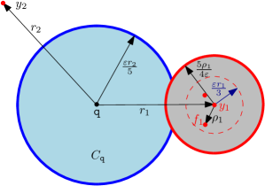
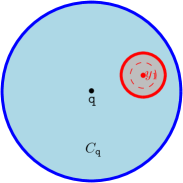
Figure 6: Examples of a computed AVD region $C_{\mathtt{q}}$.

The regions created by the algorithm in Figure 5 are the difference of two balls. An example region when the balls $\mathsf{ball}_{\mathcal{X}}\!\left({{\mathtt{q}},{{\varepsilon}r_{2}/5}}\right)$ and $\mathsf{ball}_{\mathcal{X}}\!\left({{y_{1}},{5\rho_{1}/4{\varepsilon}}}\right)$ intersect is shown in Figure 6. The intuition as to why $y_{1}$ is a valid ANN inside this region is as follows. Since the distance of $\mathtt{q}$ to $y_{1}$ is $r_{1}$, the points inside $\mathsf{ball}_{\mathcal{X}}\!\left({{y_{1}},{{\varepsilon}r_{1}/3}}\right)$ are all roughly the same distance from $\mathtt{q}$ when $\mathtt{q}$ is far enough from $y_{1}$. The next distance of interest, $\mathsf{d}_{{\mathcal{X}}}\!\left({{\mathtt{q}},{y_{2}}}\right)=r_{2}$, is the distance to a ANN of points outside this ball. As long as we are inside $\mathsf{ball}_{\mathcal{X}}\!\left({{\mathtt{q}},{{\varepsilon}r_{2}/5}}\right)$ and far enough from $y_{1}$ i.e. $\mathsf{d}_{{\mathcal{X}}}\!\left({{\mathtt{q}},{y_{1}}}\right)>5\rho_{1}/4{\varepsilon}$, the points outside $\mathsf{ball}_{\mathcal{X}}\!\left({{y_{1}},{{\varepsilon}r_{1}/3}}\right)$ are too far and cannot be a $(1+{\varepsilon})$-ANN. But if we get too close to $y_{1}$ we can no longer be certain that $y_{1}$ is a valid $(1+{\varepsilon})$-ANN, as it is no more true that distances to points inside $\mathsf{ball}_{\mathcal{X}}\!\left({{y_{1}},{{\varepsilon}r_{1}/3}}\right)$ look all roughly the same. In other words, there may be points much closer than $y_{1}$, when we are close enough to $y_{1}$. Thus in a small enough neighborhood around $y_{1}$ we need to zoom in and possibly create a new region.

6.2 Correctness

Lemma 6.1.

If $\mathsf{d}_{{\mathcal{X}}}\!\left({{\mathtt{q}},{\mathsf{p}}}\right)\geq 2\mathsf{D}^{\prime}+2\mathsf{D}^{\prime}/{\varepsilon}$ then $\mathsf{p}$ is a valid $(1+{\varepsilon})$-ANN.

Proof.

Since $\mathsf{D}^{\prime}$ is a $2$-approximation to the diameter of $\mathsf{P}$, so $2\mathsf{D}^{\prime}\geq\mathsf{D}=\mathrm{d{}i{}am}\!\left({\mathsf{P}}\right)$. This means $\mathsf{d}_{{\mathcal{X}}}\!\left({{\mathtt{q}},{\mathsf{p}}}\right)\geq\mathsf{D}+\mathsf{D}/{\varepsilon}$. Let $\mathsf{n}_{\mathtt{q}}\in\mathsf{P}$ be the closest point to $\mathtt{q}$. By the triangle inequality,

$$\mathsf{D}+\mathsf{D}/{\varepsilon}\leq\mathsf{d}_{{\mathcal{X}}}\!\left({{\mathtt{q}},{\mathsf{p}}}\right)\leq\mathsf{d}_{{\mathcal{X}}}\!\left({{\mathtt{q}},{\mathsf{n}_{\mathtt{q}}}}\right)+\mathsf{d}_{{\mathcal{X}}}\!\left({{\mathsf{n}_{\mathtt{q}}},{\mathsf{p}}}\right)\leq\mathsf{d}_{{\mathcal{X}}}\!\left({{\mathtt{q}},{\mathsf{n}_{\mathtt{q}}}}\right)+\mathsf{D}.$$

As such $\mathsf{D}\leq{\varepsilon}\mathsf{d}_{{\mathcal{X}}}\!\left({{\mathtt{q}},{\mathsf{n}_{\mathtt{q}}}}\right)$. We conclude $\mathsf{d}_{{\mathcal{X}}}\!\left({{\mathtt{q}},{\mathsf{p}}}\right)\leq\mathsf{d}_{{\mathcal{X}}}\!\left({{\mathtt{q}},{\mathsf{n}_{\mathtt{q}}}}\right)+\mathsf{d}_{{\mathcal{X}}}\!\left({{\mathsf{n}_{\mathtt{q}}},{\mathsf{p}}}\right)\leq(1+{\varepsilon})\mathsf{d}_{{\mathcal{X}}}\!\left({{\mathtt{q}},{\mathsf{n}_{\mathtt{q}}}}\right)$.

Lemma 6.2.

If there is no region in $\mathcal{R}$ containing $\mathtt{q}$ then the algorithm outputs a valid $(1+{\varepsilon}/10)$-ANN.

Proof.

We output $y_{1}$ which is a $(1+{\varepsilon}/10)$-ANN of $\mathtt{q}$.

Lemma 6.3.

The $(1+{\varepsilon}/10)$-ANN $y_{1}$ found in the algorithm is a $(1+{\varepsilon})$-ANN for any point $\overline{\mathtt{q}}\in C_{\mathtt{q}}$.

Proof.

Let $r_{1}=\mathsf{d}_{{\mathcal{X}}}\!\left({{\mathtt{q}},{y_{1}}}\right)$ and $r_{2}=\mathsf{d}_{{\mathcal{X}}}\!\left({{\mathtt{q}},{y_{2}}}\right)$. There are two possibilities.

If the region $C_{\mathtt{q}}$ is the ball $\mathsf{ball}_{\mathcal{X}}\!\left({{\mathtt{q}},{\mathsf{D}^{\prime}/4}}\right)$ constructed when there is no point in $\mathsf{P}\setminus\mathsf{ball}_{\mathcal{X}}\!\left({{y_{1}},{{\varepsilon}r_{1}/3}}\right)$, then $\mathsf{D}=\mathrm{d{}i{}am}\!\left({\mathsf{P}}\right)\leq 2{\varepsilon}r_{1}/3$. As such,

$$\mathsf{d}_{{\mathcal{X}}}\!\left({{\mathtt{q}},{\mathsf{P}}}\right)\geq\frac{\mathsf{d}_{{\mathcal{X}}}\!\left({{\mathtt{q}},{y_{1}}}\right)}{1+{\varepsilon}/10}=\frac{r_{1}}{1+{\varepsilon}/10}\geq\frac{3\mathsf{D}}{2{\varepsilon}(1+{\varepsilon}/10)}=\frac{3\mathsf{D}}{2{\varepsilon}+{\varepsilon}^{2}/5}\geq(4/3)\frac{\mathsf{D}}{{\varepsilon}}.$$

It is not hard to see that in this case, $y_{1}$ is a valid $(1+{\varepsilon})$-ANN for any point inside $\mathsf{ball}_{\mathcal{X}}\!\left({{\mathtt{q}},{\mathsf{D}^{\prime}/4}}\right)\subseteq\mathsf{ball}_{\mathcal{X}}\!\left({{\mathtt{q}},{\mathsf{D}/4}}\right)$, as $\mathsf{d}_{{\mathcal{X}}}\!\left({{\mathsf{ball}_{\mathcal{X}}\!\left({{\mathtt{q}},{\mathsf{D}/4}}\right)},{\mathsf{P}}}\right)\geq\mathsf{D}/{\varepsilon}$, for ${\varepsilon}$ sufficiently small.

Otherwise, if the set $\mathsf{P}\setminus\mathsf{ball}_{\mathcal{X}}\!\left({{y_{1}},{{\varepsilon}r_{1}/3}}\right)$ is nonempty then let $y_{2}$ be a $(1+{\varepsilon}/10)$-ANN of $\mathtt{q}$ in $\mathsf{P}\setminus\mathsf{ball}_{\mathcal{X}}\!\left({{y_{1}},{{\varepsilon}r_{1}/3}}\right)$ and let $r_{2}=\mathsf{d}_{{\mathcal{X}}}\!\left({{\mathtt{q}},{y_{2}}}\right)$. We break the analysis into two cases.

1. If $r_{2}\leq 2r_{1}$, then let $\overline{\mathtt{q}}$ be any point in $C_{\mathtt{q}}$ and let $\mathsf{n}_{\overline{\mathtt{q}}}\in\mathsf{P}$ be its nearest neighbor. If $\mathsf{n}_{\overline{\mathtt{q}}}=y_{1}$ there is nothing to show. Otherwise $\mathsf{d}_{{\mathcal{X}}}\!\left({{\mathtt{q}},{\overline{\mathtt{q}}}}\right)\leq{\varepsilon}r_{2}/5$ and by the triangle inequality we have

   $$\mathsf{d}_{{\mathcal{X}}}\!\left({{\overline{\mathtt{q}}},{\mathsf{n}_{\overline{\mathtt{q}}}}}\right) \geq\mathsf{d}_{{\mathcal{X}}}\!\left({{\mathtt{q}},{\mathsf{n}_{\overline{\mathtt{q}}}}}\right)-\mathsf{d}_{{\mathcal{X}}}\!\left({{\mathtt{q}},{\overline{\mathtt{q}}}}\right)\geq\mathsf{d}_{{\mathcal{X}}}\!\left({{\mathtt{q}},{\mathsf{n}_{\overline{\mathtt{q}}}}}\right)-{\varepsilon}r_{2}/5$$

   $$\geq\mathsf{d}_{{\mathcal{X}}}\!\left({{\mathtt{q}},{y_{1}}}\right)/(1+{\varepsilon}/10)-{\varepsilon}2r_{1}/5$$

   $$\geq(1-{\varepsilon}/2)r_{1},$$

   as $\mathsf{d}_{{\mathcal{X}}}\!\left({{\mathtt{q}},{\mathsf{n}_{\overline{\mathtt{q}}}}}\right)\geq\mathsf{d}_{{\mathcal{X}}}\!\left({{\mathtt{q}},{\mathsf{P}}}\right)\geq\mathsf{d}_{{\mathcal{X}}}\!\left({{\mathtt{q}},{y_{1}}}\right)/(1+{\varepsilon}/10)$ and $r_{1}=\mathsf{d}_{{\mathcal{X}}}\!\left({{\mathtt{q}},{y_{1}}}\right)$. Again, by the triangle inequality and the above, we have

   $$\mathsf{d}_{{\mathcal{X}}}\!\left({{\overline{\mathtt{q}}},{y_{1}}}\right) \leq\mathsf{d}_{{\mathcal{X}}}\!\left({{\mathtt{q}},{y_{1}}}\right)+\mathsf{d}_{{\mathcal{X}}}\!\left({{\mathtt{q}},{\overline{\mathtt{q}}}}\right)\leq\mathsf{d}_{{\mathcal{X}}}\!\left({{\mathtt{q}},{y_{1}}}\right)+2{\varepsilon}r_{1}/5=(1+2{\varepsilon}/5)r_{1}$$

   $$\leq\frac{1+2{\varepsilon}/5}{1-{\varepsilon}/2}\mathsf{d}_{{\mathcal{X}}}\!\left({{\overline{\mathtt{q}}},{\mathsf{n}_{\overline{\mathtt{q}}}}}\right)\leq(1+{\varepsilon})\mathsf{d}_{{\mathcal{X}}}\!\left({{\overline{\mathtt{q}}},{\mathsf{n}_{\overline{\mathtt{q}}}}}\right),$$

   for ${\varepsilon}\leq 1/5$.

2. If $r_{2}>2r_{1}$ then let $f_{1}$ be the furthest point from $y_{1}$ inside $\mathsf{ball}_{\mathcal{X}}\!\left({{y_{1}},{{\varepsilon}r_{1}/3}}\right)$ and let $\rho_{1}=\mathsf{d}_{{\mathcal{X}}}\!\left({{y_{1}},{f_{1}}}\right)$. Let $\overline{\mathtt{q}}$ be any point in $C_{\mathtt{q}}$ and as before let $\mathsf{n}_{\overline{\mathtt{q}}}\in\mathsf{P}$ be its nearest neighbor. We claim that the nearest neighbor of $\overline{\mathtt{q}}$ in $\mathsf{P}$ lies in $\mathsf{ball}_{\mathcal{X}}\!\left({{y_{1}},{\rho_{1}}}\right)$. To see this, let $z$ be any point in $\mathsf{P}\setminus\mathsf{ball}_{\mathcal{X}}\!\left({{y_{1}},{\rho_{1}}}\right)$. Noting that the distance from $\mathtt{q}$ to the closest point in $\mathsf{P}$ outside $\mathsf{ball}_{\mathcal{X}}\!\left({{y_{1}},{\rho_{1}}}\right)$ is at least $r_{2}/(1+{\varepsilon}/10)$ and by triangle inequality we have,

   $$\mathsf{d}_{{\mathcal{X}}}\!\left({{\overline{\mathtt{q}}},{z}}\right) \geq\mathsf{d}_{{\mathcal{X}}}\!\left({{\mathtt{q}},{z}}\right)-\mathsf{d}_{{\mathcal{X}}}\!\left({{\mathtt{q}},{\overline{\mathtt{q}}}}\right)\geq\mathsf{d}_{{\mathcal{X}}}\!\left({{\mathtt{q}},{z}}\right)-{\varepsilon}r_{2}/5$$

   $$\geq r_{2}/(1+{\varepsilon}/10)-{\varepsilon}r_{2}/5>(1-3{\varepsilon}/10)r_{2}.$$

   On the other hand, as $r_{1}=\mathsf{d}_{{\mathcal{X}}}\!\left({{\mathtt{q}},{y_{1}}}\right)$ and $r_{1}<r_{2}/2$, we have

   $$\mathsf{d}_{{\mathcal{X}}}\!\left({{\overline{\mathtt{q}}},{y_{1}}}\right) \leq\mathsf{d}_{{\mathcal{X}}}\!\left({{\mathtt{q}},{y_{1}}}\right)+\mathsf{d}_{{\mathcal{X}}}\!\left({{\mathtt{q}},{\overline{\mathtt{q}}}}\right)\leq\mathsf{d}_{{\mathcal{X}}}\!\left({{\mathtt{q}},{y_{1}}}\right)+{\varepsilon}r_{2}/5=r_{1}+{\varepsilon}r_{2}/5<r_{2}/2+{\varepsilon}r_{2}/5$$

   $$\leq(1-3{\varepsilon}/10)r_{2}<\mathsf{d}_{{\mathcal{X}}}\!\left({{\overline{\mathtt{q}}},{z}}\right),$$

   by the above. As such, no point in $\mathsf{P}\setminus\mathsf{ball}_{\mathcal{X}}\!\left({{y_{1}},{\rho_{1}}}\right)$ can be the nearest neighbor of $\overline{\mathtt{q}}$ for ${\varepsilon}<1$. As such $\mathsf{n}_{\overline{\mathtt{q}}}\in\mathsf{ball}_{\mathcal{X}}\!\left({{y_{1}},{\rho_{1}}}\right)$. Now,

   $$\mathsf{d}_{{\mathcal{X}}}\!\left({{\overline{\mathtt{q}}},{y_{1}}}\right)\leq\mathsf{d}_{{\mathcal{X}}}\!\left({{\overline{\mathtt{q}}},{\mathsf{n}_{\overline{\mathtt{q}}}}}\right)+\mathsf{d}_{{\mathcal{X}}}\!\left({{\mathsf{n}_{\overline{\mathtt{q}}}},{y_{1}}}\right)\leq\mathsf{d}_{{\mathcal{X}}}\!\left({{\overline{\mathtt{q}}},{\mathsf{n}_{\overline{\mathtt{q}}}}}\right)+\rho_{1}.$$ (1)

   Now $\overline{\mathtt{q}}\in C_{\mathtt{q}}=\mathsf{ball}_{\mathcal{X}}\!\left({{\mathtt{q}},{{\varepsilon}r_{2}/5}}\right)\setminus\mathsf{ball}_{\mathcal{X}}\!\left({{y_{1}},{5\rho_{1}/4{\varepsilon}}}\right)$, and thus $\mathsf{d}_{{\mathcal{X}}}\!\left({{\overline{\mathtt{q}}},{y_{1}}}\right)>5\rho_{1}/4{\varepsilon}$. Thus,

   $$\mathsf{d}_{{\mathcal{X}}}\!\left({{\overline{\mathtt{q}}},{\mathsf{n}_{\overline{\mathtt{q}}}}}\right)\geq\mathsf{d}_{{\mathcal{X}}}\!\left({{\overline{\mathtt{q}}},{y_{1}}}\right)-\mathsf{d}_{{\mathcal{X}}}\!\left({{y_{1}},{\mathsf{n}_{\overline{\mathtt{q}}}}}\right)\geq\mathsf{d}_{{\mathcal{X}}}\!\left({{\overline{\mathtt{q}}},{y_{1}}}\right)-\rho_{1}\geq\!\left({\frac{5}{4{\varepsilon}}-1}\right)\rho_{1}.$$ (2)

   Therefore from (1) and (2), we have

   $$\mathsf{d}_{{\mathcal{X}}}\!\left({{\overline{\mathtt{q}}},{y_{1}}}\right) \leq\mathsf{d}_{{\mathcal{X}}}\!\left({{\overline{\mathtt{q}}},{\mathsf{n}_{\overline{\mathtt{q}}}}}\right)+\rho_{1}\leq\!\left({\rule[0.0pt]{0.0pt}{9.95863pt}1+\frac{1}{5/4{\varepsilon}-1}}\right)\mathsf{d}_{{\mathcal{X}}}\!\left({{\overline{\mathtt{q}}},{\mathsf{n}_{\overline{\mathtt{q}}}}}\right)=\!\left({\rule[0.0pt]{0.0pt}{9.95863pt}1+\frac{4{\varepsilon}}{5-4{\varepsilon}}}\right)\mathsf{d}_{{\mathcal{X}}}\!\left({{\overline{\mathtt{q}}},{\mathsf{n}_{\overline{\mathtt{q}}}}}\right)$$

   $$\leq(1+{\varepsilon})\mathsf{d}_{{\mathcal{X}}}\!\left({{\overline{\mathtt{q}}},{\mathsf{n}_{\overline{\mathtt{q}}}}}\right).$$

   for ${\varepsilon}\leq 1/4$.

6.3 Bounding the number of regions created

The online algorithm presented in Figure 5 is valid for any general metric space $\mathcal{X}$, without any restriction on the subspace of query points. However, when the query points are restricted to lie in a subspace $\mathcal{M}$ of low doubling dimension $\tau$, then one can show that at most $n{\varepsilon}^{-O\left({{\tau}}\right)}$ regions are created overall, where $n=\left\lvert{\mathsf{P}}\right\rvert$. There are two types of regions created. The outer regions are created when $\mathsf{P}\setminus\mathsf{ball}_{\mathcal{X}}\!\left({{y_{1}},{{\varepsilon}r_{1}/3}}\right)$ is empty and the inner regions are created when this condition does not hold. An example of an inner region is shown in Figure 6.

6.3.1 Bounding the number of outer regions

First we show that there are at most ${\varepsilon}^{-O\left({{\tau}}\right)}$ outer regions created.

Lemma 6.4.

When all the queries to the algorithm come from a subspace of doubling dimension $\tau$, then at most ${\varepsilon}^{-O\left({{\tau}}\right)}$ outer regions are created overall.

Proof.

Any two query points creating distinct outer regions occur at a distance of at least $\mathsf{D}^{\prime}/4$ from each other. However all of them occur inside a ball of radius $4\mathsf{D}^{\prime}/{\varepsilon}$ around $\mathsf{p}$. Thus the spread of the set containing all these query points is bounded by $\!\left({4\mathsf{D}^{\prime}/{\varepsilon}}\right)\,/\,\left({\mathsf{D}^{\prime}/4}\right)=O(1/{\varepsilon})$. As such, there are at most ${\varepsilon}^{-O\left({{\tau}}\right)}$ such points.

6.3.2 Bounding the number of inner regions

We now consider the inner regions created by the algorithm. Consider the mapped point set $\mathsf{P}^{\prime}$ in the space $\mathcal{M}^{\prime}$, see Section 2.3. Fix a $c$-WSPD $\left\{{\rule[0.0pt]{0.0pt}{9.95863pt}\!\left\{{A_{1}^{\prime},B_{1}^{\prime}}\right\},\dots,\left\{{A_{s}^{\prime},B_{s}^{\prime}}\right\}}\right\}$ of $\mathsf{P}^{\prime}$ where $c$ is a constant to be specified shortly and $s=c^{O\left({{\tau}}\right)}n$ is the number of pairs. Let $A_{i},B_{i}\subseteq\mathsf{P}$ denote the corresponding “unmapped” points corresponding to $A_{i}^{\prime},B_{i}^{\prime}$, that is, $A_{i}=\left\{{\mathsf{p}\in\mathsf{P}~{}|~{}\mathsf{p}^{\prime}\in A_{i}^{\prime}}\right\}$ and $B_{i}=\left\{{\mathsf{p}\in\mathsf{P}~{}|~{}\mathsf{p}^{\prime}\in B_{i}^{\prime}}\right\}$. If a query point $\mathtt{q}$ creates a new inner region we shall assign it to a set $\mathcal{U}_{i}$ associated with the pair $\left\{{A_{i}^{\prime},B_{i}^{\prime}}\right\}$, if the pair of points $y_{1}^{\prime},y_{2}^{\prime}$ of the algorithm satisfy $y_{1}^{\prime}\in A_{i}^{\prime}$ and $y_{2}^{\prime}\in B_{i}^{\prime}$. Similarly assign $\mathtt{q}$ to the set $\mathcal{V}_{i}$ if $y_{1}^{\prime}\in B_{i}^{\prime}$ and $y_{2}^{\prime}\in A_{i}^{\prime}$.

Thus, the query points that gave rise to new regions are now associated with pairs of the WSPD. Our analysis bounds the size of the sets $\mathcal{U}_{i}$ and $\mathcal{V}_{i}$ associated with a pair $\left\{{A_{i}^{\prime},B_{i}^{\prime}}\right\}$, for $i=1,\ldots,s$, thus bounding the total number of regions created.

Let $\mathcal{U}_{i}^{\prime}=\left\{{\mathtt{q}^{\prime}\,\left|\,{\mathtt{q}\in\mathcal{U}_{i}}\rule[-5.69046pt]{0.0pt}{11.38092pt}\right.}\right\}\subseteq\mathcal{M}^{\prime}$ and $\mathcal{V}_{i}^{\prime}=\left\{{\mathtt{q}^{\prime}\,\left|\,{\mathtt{q}\in\mathcal{V}_{i}}\rule[-5.69046pt]{0.0pt}{11.38092pt}\right.}\right\}$, for $i=1,\ldots,s$. For a pair $\left\{{A_{i}^{\prime},B_{i}^{\prime}}\right\}$ of the WSPD we define the numbers $\mathsf{h}_{\max}\!\left({A_{i}^{\prime}}\right)=\max_{(u,h)\in A_{i}^{\prime}}h$. Similarly let $\mathsf{h}_{\max}\!\left({B_{i}^{\prime}}\right)=\max_{(z,h)\in B_{i}^{\prime}}h$. Also, let

$$\mathsf{l}_{i}=\max_{u^{\prime}\in A_{i}^{\prime},z^{\prime}\in B_{i}^{\prime}}\mathsf{d}_{{\mathcal{X}}}\!\left({{\alpha({u})},{\alpha({z})}}\right)\qquad\text{ and }\qquad\mathsf{L}_{i}=\mathsf{l}_{i}+\mathsf{h}_{\max}\!\left({A_{i}^{\prime}}\right)+\mathsf{h}_{\max}\!\left({B_{i}^{\prime}}\right).$$

The following sequence of lemmas establish our claim. The basic strategy is to show that the set $\mathcal{U}_{i}^{\prime}$ has spread $O\!\left({{1/{\varepsilon}^{2}}}\right)$. This holds analogously for $\mathcal{V}_{i}^{\prime}$ and so we will only work with $\mathcal{U}_{i}^{\prime}$. We will assume that $c$ is a sufficiently large constant and ${\varepsilon}$ is sufficiently small.

Lemma 6.5.

For any $i$, we have $\mathrm{d{}i{}am}_{\mathcal{M}^{\prime}}\!\left({A_{i}^{\prime}}\right)\leq\mathsf{L}_{i}/c$ and $\mathrm{d{}i{}am}_{\mathcal{M}^{\prime}}\!\left({B_{i}^{\prime}}\right)\leq\mathsf{L}_{i}/c$.

Proof.

By the construction of the WSPD, we have that $\mathrm{d{}i{}am}_{\mathcal{M}^{\prime}}\!\left({A_{i}^{\prime}}\right)\leq\mathsf{d}_{{\mathcal{M}^{\prime}}}\!\left({{A_{i}^{\prime}},{B_{i}^{\prime}}}\right)/c$. Moreover, we have

$$\mathsf{d}_{{\mathcal{M}^{\prime}}}\!\left({{A_{i}^{\prime}},{B_{i}^{\prime}}}\right) =\min_{\mathsf{p}^{\prime}\in A_{i}^{\prime},v^{\prime}\in B_{i}^{\prime}}\mathsf{d}_{{\mathcal{M}^{\prime}}}\!\left({{\mathsf{p}^{\prime}},{v^{\prime}}}\right)=\min_{\mathsf{p}^{\prime}\in A_{i}^{\prime},v^{\prime}\in B_{i}^{\prime}}\!\left({\rule[-5.69046pt]{0.0pt}{11.38092pt}\mathsf{d}_{{\mathcal{X}}}\!\left({{\rule[0.0pt]{0.0pt}{9.95863pt}\alpha({\mathsf{p}})},{\alpha({v})}}\right)+\left\lvert{0pt{\mathsf{p}}-0pt{v}}\right\rvert}\right)$$

$$\leq\,\mathsf{l}_{i}+\min_{\mathsf{p}^{\prime}\in A_{i}^{\prime},v^{\prime}\in B_{i}^{\prime}}\!\left({\rule[-5.69046pt]{0.0pt}{11.38092pt}\left\lvert{0pt{\mathsf{p}}}\right\rvert+\left\lvert{0pt{v}}\right\rvert}\right)\leq\mathsf{l}_{i}+\mathsf{h}_{\max}\!\left({A_{i}^{\prime}}\right)+\mathsf{h}_{\max}\!\left({B_{i}^{\prime}}\right)=\mathsf{L}_{i}.$$

This implies that $\mathrm{d{}i{}am}_{\mathcal{M}^{\prime}}\!\left({A_{i}^{\prime}}\right)\leq\mathsf{L}_{i}/c$, and similarly $\mathrm{d{}i{}am}_{\mathcal{M}^{\prime}}\!\left({B_{i}^{\prime}}\right)\leq\mathsf{L}_{i}/c$.

Lemma 6.6.

We have $\mathsf{diam}\!\left({{\mathcal{U}_{i}^{\prime}}}\right)=O\!\left({{\mathsf{L}_{i}/{\varepsilon}}}\right)$.

Proof.

Let $\mathtt{q}$ be a (query) point in $\mathcal{U}_{i}$. By assumption we have $y_{1}^{\prime}\in A_{i}^{\prime}$ and $y_{2}^{\prime}\in B_{i}^{\prime}$. By the triangle inequality,

$$\mathsf{d}_{{\mathcal{X}}}\!\left({{y_{1}},{y_{2}}}\right) \leq\mathsf{d}_{{\mathcal{X}}}\!\left({{y_{1}},{\alpha({y_{1}})}}\right)+\mathsf{d}_{{\mathcal{X}}}\!\left({{\alpha({y_{1}})},{\alpha({y_{2}})}}\right)+\mathsf{d}_{{\mathcal{X}}}\!\left({{\alpha({y_{2}})},{y_{2}}}\right)\leq\mathsf{h}_{\max}\!\left({A_{i}^{\prime}}\right)+\mathsf{l}_{i}+\mathsf{h}_{\max}\!\left({B_{i}^{\prime}}\right)$$

$$\leq\mathsf{L}_{i}.$$

On the other hand, since the point $y_{2}$ is outside $\mathsf{ball}_{\mathcal{X}}\!\left({{y_{1}},{{\varepsilon}r_{1}/3}}\right)$, we have that $\mathsf{d}_{{\mathcal{X}}}\!\left({{y_{1}},{y_{2}}}\right)>{\varepsilon}r_{1}/3$, where $r_{1}=\mathsf{d}_{{\mathcal{X}}}\!\left({{\mathtt{q}},{y_{1}}}\right)$. This gives us $r_{1}<(3/{\varepsilon})\mathsf{d}_{{\mathcal{X}}}\!\left({{y_{1}},{y_{2}}}\right)<3\mathsf{L}_{i}/{\varepsilon}$. By Lemma 2.4, $\mathsf{d}_{{\mathcal{M}^{\prime}}}\!\left({{\mathtt{q}^{\prime}},{y_{1}^{\prime}}}\right)\leq 3\mathsf{d}_{{\mathcal{X}}}\!\left({{\mathtt{q}},{y_{1}}}\right)=3r_{1}<9\mathsf{L}_{i}/{\varepsilon}$. Also, we have,

$$\mathsf{d}_{{\mathcal{M}^{\prime}}}\!\left({{y_{1}^{\prime}},{y_{2}^{\prime}}}\right) =\mathsf{d}_{{\mathcal{X}}}\!\left({{\alpha({y_{1}})},{\alpha({y_{2}})}}\right)+\left|{0pt{y_{1}}-0pt{y_{2}}}\right|\leq\mathsf{l}_{i}+\mathsf{h}_{\max}\!\left({A_{i}^{\prime}}\right)+\mathsf{h}_{\max}\!\left({B_{i}^{\prime}}\right)=\mathsf{L}_{i}.$$ (3)

Let $\overline{\mathtt{q}}$ be any other point in $\mathcal{U}_{i}$, and let the points $\overline{y_{1}\!}$ and $\overline{y_{2}\!}\,$ be the points found by the algorithm such that $\overline{y_{1}\!}^{\prime}\in A_{i}^{\prime}$ and $\overline{y_{2}\!}\,^{\prime}\in B_{i}^{\prime}$. Since $y_{1}^{\prime}$ is also in $A_{i}^{\prime}$, we have by Lemma 6.5 that $\mathsf{d}_{{\mathcal{M}^{\prime}}}\!\left({{y_{1}^{\prime}},{\overline{y_{1}\!}^{\prime}}}\right)\leq\mathrm{d{}i{}am}_{\mathcal{M}^{\prime}}\!\left({A_{i}}\right)\leq\mathsf{L}_{i}/c$. As such,

$$\mathsf{diam}\!\left({{\mathcal{U}_{i}^{\prime}}}\right) =\max\limits_{\mathtt{q}^{\prime},\overline{\mathtt{q}}^{\prime}\in\mathcal{U}_{i}^{\prime}}\mathsf{d}_{{\mathcal{M}^{\prime}}}\!\left({{\mathtt{q}^{\prime}},{\overline{\mathtt{q}}^{\prime}}}\right)\leq\max\limits_{\mathtt{q}^{\prime},\overline{\mathtt{q}}^{\prime}\in\mathcal{U}_{i}^{\prime}}(\mathsf{d}_{{\mathcal{M}^{\prime}}}\!\left({{\mathtt{q}^{\prime}},{y_{1}^{\prime}}}\right)+\mathsf{d}_{{\mathcal{M}^{\prime}}}\!\left({{y_{1}^{\prime}},{\overline{y_{1}\!}^{\prime}}}\right)+\mathsf{d}_{{\mathcal{M}^{\prime}}}\!\left({{\overline{\mathtt{q}}^{\prime}},{\overline{y_{1}\!}^{\prime}}}\right))$$

$$\leq 9\mathsf{L}_{i}/{\varepsilon}+\mathsf{L}_{i}/c+9\mathsf{L}_{i}/{\varepsilon}=O\!\left({{\mathsf{L}_{i}/{\varepsilon}}}\right),$$

for ${\varepsilon}$ small enough.

Lemma 6.7.

For a query point $\mathtt{q}$, the associated distances $r_{2}$ and $\mathsf{L}_{i}$ satisfy $r_{2}\geq\mathsf{L}_{i}/18$.

Proof.

Let $u^{\prime}$ be the point with maximum height in $A_{i}^{\prime}$; that is $0pt{u}=\mathsf{h}_{\max}\!\left({A_{i}^{\prime}}\right)$. By Lemma 6.5, we have $\mathsf{d}_{{\mathcal{M}^{\prime}}}\!\left({{u^{\prime}},{y_{1}^{\prime}}}\right)\leq\mathsf{L}_{i}/c$. The definition of the distance in $\mathcal{M}^{\prime}$, gives

$$\mathsf{h}_{\max}\!\left({A_{i}^{\prime}}\right)-0pt{y_{1}}\leq\left\lvert{\mathsf{h}_{\max}\!\left({A_{i}^{\prime}}\right)-0pt{y_{1}}}\right\rvert=\left\lvert{0pt{u}-0pt{y_{1}}}\right\rvert\leq\mathsf{d}_{{\mathcal{M}^{\prime}}}\!\left({{u^{\prime}},{y_{1}^{\prime}}}\right)\leq\mathsf{L}_{i}/c,$$

and so $0pt{y_{1}}\geq\mathsf{h}_{\max}\!\left({A_{i}^{\prime}}\right)-\mathsf{L}_{i}/c$. Similarly we have, $0pt{y_{2}}\geq\mathsf{h}_{\max}\!\left({B_{i}^{\prime}}\right)-\mathsf{L}_{i}/c$. We have $r_{1}=\mathsf{d}_{{\mathcal{X}}}\!\left({{\mathtt{q}},{y_{1}}}\right)\geq\mathsf{d}_{{\mathcal{X}}}\!\left({{y_{1}},{\mathcal{M}}}\right)=\mathsf{d}_{{\mathcal{X}}}\!\left({{y_{1}},{\alpha({y_{1}})}}\right)=0pt{y_{1}}$ and similarly $r_{2}=\mathsf{d}_{{\mathcal{X}}}\!\left({{\mathtt{q}},{y_{2}}}\right)\geq 0pt{y_{2}}$. Noting that, $r_{2}\geq\mathsf{d}_{{\mathcal{X}}}\!\left({{\mathtt{q}},{\mathsf{P}}}\right)\geq r_{1}/(1+{\varepsilon}/10)\geq(10/11)r_{1}$ we get,

$$2.1r_{2}=r_{2}+\frac{11}{10}r_{2}\geq r_{2}+r_{1}\geq 0pt{y_{2}}+0pt{y_{1}}\geq\mathsf{h}_{\max}\!\left({A_{i}^{\prime}}\right)+\mathsf{h}_{\max}\!\left({B_{i}^{\prime}}\right)-\frac{2\mathsf{L}_{i}}{c}.$$ (4)

Let $z^{\prime}\in A_{i}^{\prime}$ and $w^{\prime}\in B_{i}^{\prime}$ be such that $\mathsf{d}_{{\mathcal{X}}}\!\left({{\alpha({z})},{\alpha({w})}}\right)=\mathsf{l}_{i}$. Observing that $\mathsf{d}_{{\mathcal{M}^{\prime}}}\!\left({{\mathtt{q}^{\prime}},{y_{1}^{\prime}}}\right)\leq 3\mathsf{d}_{{\mathcal{X}}}\!\left({{\mathtt{q}},{y_{1}}}\right)=3r_{1}$ and similarly $\mathsf{d}_{{\mathcal{M}^{\prime}}}\!\left({{\mathtt{q}^{\prime}},{y_{2}^{\prime}}}\right)\leq 3\mathsf{d}_{{\mathcal{X}}}\!\left({{\mathtt{q}},{y_{2}}}\right)=3r_{2}$, we have by the triangle inequality that

$$\mathsf{d}_{{\mathcal{M}^{\prime}}}\!\left({{\mathtt{q}^{\prime}},{z^{\prime}}}\right)\leq\mathsf{d}_{{\mathcal{M}^{\prime}}}\!\left({{\mathtt{q}^{\prime}},{y_{1}^{\prime}}}\right)+\mathsf{d}_{{\mathcal{M}^{\prime}}}\!\left({{y_{1}^{\prime}},{z^{\prime}}}\right)\leq 3r_{1}+\mathrm{d{}i{}am}\!\left({A_{i}^{\prime}}\right)\leq 3r_{1}+\mathsf{L}_{i}/c,$$

and $$\mathsf{d}_{{\mathcal{M}^{\prime}}}\!\left({{\mathtt{q}^{\prime}},{w^{\prime}}}\right)\leq\mathsf{d}_{{\mathcal{M}^{\prime}}}\!\left({{\mathtt{q}^{\prime}},{y_{2}^{\prime}}}\right)+\mathsf{d}_{{\mathcal{M}^{\prime}}}\!\left({{y_{2}^{\prime}},{w^{\prime}}}\right)\leq 3r_{2}+\mathrm{d{}i{}am}\!\left({B_{i}^{\prime}}\right)\leq 3r_{2}+\mathsf{L}_{i}/c,$$

by Lemma 6.5. By the triangle inequality, we have

$$\mathsf{l}_{i} \leq\mathsf{d}_{{\mathcal{M}^{\prime}}}\!\left({{z^{\prime}},{w^{\prime}}}\right)\leq\mathsf{d}_{{\mathcal{M}^{\prime}}}\!\left({{z^{\prime}},{\mathtt{q}^{\prime}}}\right)+\mathsf{d}_{{\mathcal{M}^{\prime}}}\!\left({{\mathtt{q}^{\prime}},{w^{\prime}}}\right)\leq 3r_{1}+3r_{2}+\frac{2\mathsf{L}_{i}}{c}\leq 6.3r_{2}+\frac{2\mathsf{L}_{i}}{c},$$

as $r_{1}\leq(11/10)r_{2}$. Thus we have,

$$6.3r_{2}\geq\mathsf{l}_{i}-\frac{2\mathsf{L}_{i}}{c}.$$ (5)

By Eq. (4) and Eq. (5), we have, for $c\geq 8$, that

$$9r_{2}\geq 2.1r_{2}+6.3r_{2} \geq\!\left({\mathsf{h}_{\max}\!\left({A_{i}^{\prime}}\right)+\mathsf{h}_{\max}\!\left({B_{i}^{\prime}}\right)-\frac{2\mathsf{L}_{i}}{c}}\right)+\!\left({\mathsf{l}_{i}-\frac{2\mathsf{L}_{i}}{c}}\right)$$

$$=\mathsf{h}_{\max}\!\left({A_{i}^{\prime}}\right)+\mathsf{h}_{\max}\!\left({B_{i}^{\prime}}\right)+\mathsf{l}_{i}-\frac{4\mathsf{L}_{i}}{c}\geq\mathsf{L}_{i}-\frac{\mathsf{L}_{i}}{2}=\frac{\mathsf{L}_{i}}{2},$$

which implies $\mathsf{L}_{i}\leq 18r_{2}$.

Suppose $\overline{\mathtt{q}}$ was added to $\mathcal{U}_{i}$ after $\mathtt{q}$. We want to show that for $\mathtt{q},\overline{\mathtt{q}}\in\mathcal{U}_{i}$ we must have $\mathsf{d}_{{\mathcal{M}^{\prime}}}\!\left({{\mathtt{q}^{\prime}},{\overline{\mathtt{q}}^{\prime}}}\right)>{\varepsilon}r_{2}/5$ where $r_{2}=\mathsf{d}_{{\mathcal{X}}}\!\left({{\mathtt{q}},{y_{2}}}\right)$. We establish this through a sequence of lemmas. The proof is essentially by contradiction, and the next four lemmas assume the contrary to derive a contradiction. Roughly speaking, the assumption that $\mathsf{d}_{{\mathcal{M}^{\prime}}}\!\left({{\mathtt{q}^{\prime}},{\overline{\mathtt{q}}^{\prime}}}\right)=\mathsf{d}_{{\mathcal{X}}}\!\left({{\mathtt{q}},{\overline{\mathtt{q}}}}\right)\leq{\varepsilon}r_{2}/5$ places $\overline{\mathtt{q}}$ in the chipped off region of the crescent region $C_{\mathtt{q}}$. It turns out that $\overline{\mathtt{q}}$ is far from both the approximate nearest neighbor of $\mathtt{q}$, which is $y_{1}$ and the approximate nearest neighbor of $\mathtt{q}$ outside an environ of $y_{1}$, which is $y_{2}$. Under the assumption $\mathtt{q},\overline{\mathtt{q}}\in\mathcal{U}_{i}$ we should however be able to find the corresponding approximate nearest neighbors for $\overline{\mathtt{q}}$ close to those of $\mathtt{q}$. Enforcing the constraint that the approximate nearest neighbor of $\overline{\mathtt{q}}$ cannot be the second approximate nearest neighbor of $\mathtt{q}$, which is $y_{2}$, leads to either counting discrepancies or geometric contradictions arising from the triangle inequality.

Lemma 6.8.

Let $\mathtt{q},\overline{\mathtt{q}}$ be two points of $\mathcal{U}_{i}$, such that $\overline{\mathtt{q}}$ was added after $\mathtt{q}$. If $\mathsf{d}_{{\mathcal{X}}}\!\left({{\mathtt{q}},{\overline{\mathtt{q}}}}\right)\leq{\varepsilon}r_{2}/5$, then (i) $\mathsf{d}_{{\mathcal{X}}}\!\left({{\overline{\mathtt{q}}},{y_{1}}}\right)\leq(5/4{\varepsilon})\rho_{1}$, and (ii) $r_{2}\geq(2/{\varepsilon})r_{1}$.

Proof.

Since $\overline{\mathtt{q}}$ created a new region it lies outside $C_{\mathtt{q}}=\mathsf{ball}_{\mathcal{X}}\!\left({{\mathtt{q}},{{\varepsilon}r_{2}/5}}\right)\setminus\mathsf{ball}_{\mathcal{X}}\!\left({{y_{1}},{5\rho_{1}/4{\varepsilon}}}\right)$. Since by assumption $\overline{\mathtt{q}}\in\mathsf{ball}_{\mathcal{X}}\!\left({{\mathtt{q}},{{\varepsilon}r_{2}/5}}\right)$, it must be the case that $\overline{\mathtt{q}}\in\mathsf{ball}_{\mathcal{X}}\!\left({{y_{1}},{5\rho_{1}/4{\varepsilon}}}\right)$, as otherwise $\overline{\mathtt{q}}\in C_{\mathtt{q}}$. Thus, these two balls intersect, and

$$\frac{{\varepsilon}}{5}r_{2}+\frac{5}{4{\varepsilon}}\rho_{1}\geq\mathsf{d}_{{\mathcal{X}}}\!\left({{\mathtt{q}},{y_{1}}}\right)=r_{1}.$$

But $\rho_{1}\leq{\varepsilon}r_{1}/3$ and so $r_{1}\geq(3/{\varepsilon})\rho_{1}$, implying

$$\frac{{\varepsilon}}{5}r_{2}+\frac{5}{12}r_{1}\geq\frac{{\varepsilon}}{5}r_{2}+\frac{5}{12}\cdot\frac{3}{{\varepsilon}}\rho_{1}=\frac{{\varepsilon}}{5}r_{2}+\frac{5}{4{\varepsilon}}\rho_{1}\geq r_{1}\quad\implies\quad r_{2}\geq\frac{35}{12{\varepsilon}}r_{1}\geq\frac{2}{{\varepsilon}}r_{1}.$$

Lemma 6.9.

Let $\mathtt{q},\overline{\mathtt{q}}$ be two points in $\mathcal{U}_{i}$ such that $\overline{\mathtt{q}}$ was added after $\mathtt{q}$. If $\mathsf{d}_{{\mathcal{X}}}\!\left({{\mathtt{q}},{\overline{\mathtt{q}}}}\right)\leq{\varepsilon}r_{2}/5$ then, for sufficiently small ${\varepsilon}$ and sufficiently large $c$, we have that

1. $r_{1}\leq{\varepsilon}\mathsf{L}_{i}$.

2. $\mathsf{d}_{{\mathcal{X}}}\!\left({{y_{1}},{\overline{\mathtt{q}}}}\right)\leq 5r_{1}/12\leq{\varepsilon}\mathsf{L}_{i}$.

3. $\mathsf{d}_{{\mathcal{X}}}\!\left({{\overline{\mathtt{q}}},{B_{i}}}\right)\geq\mathsf{L}_{i}/120$.

Proof.

(A) By Eq. (3) we have $\mathsf{d}_{{\mathcal{M}^{\prime}}}\!\left({{y_{1}^{\prime}},{y_{2}^{\prime}}}\right)\leq\mathsf{L}_{i}$. Now, by Lemma 6.8, we have $r_{2}\geq(2/{\varepsilon})r_{1}$. As such, by the triangle inequality, and by Lemma 2.4, we have $\displaystyle\mathsf{L}_{i}$ $\displaystyle\geq\mathsf{d}_{{\mathcal{M}^{\prime}}}\!\left({{y_{1}^{\prime}},{y_{2}^{\prime}}}\right)\geq\mathsf{d}_{{\mathcal{M}^{\prime}}}\!\left({{\mathtt{q}^{\prime}},{y_{2}^{\prime}}}\right)-\mathsf{d}_{{\mathcal{M}^{\prime}}}\!\left({{\mathtt{q}^{\prime}},{y_{1}^{\prime}}}\right)\geq\mathsf{d}_{{\mathcal{X}}}\!\left({{\mathtt{q}},{y_{2}}}\right)-3\mathsf{d}_{{\mathcal{X}}}\!\left({{\mathtt{q}},{y_{1}}}\right)$ (6) $\displaystyle\geq r_{2}-3r_{1}\geq 2r_{1}/{\varepsilon}-3r_{1}\geq r_{1}/{\varepsilon},$ for ${\varepsilon}\leq 1/3$. Thus $\mathsf{L}_{i}\geq r_{1}/{\varepsilon}$. (B) In terms of $r_{2}$, by Eq. (6), we have $\displaystyle\mathsf{d}_{{\mathcal{M}^{\prime}}}\!\left({{y_{1}^{\prime}},{y_{2}^{\prime}}}\right)$ $\displaystyle\geq r_{2}-3r_{1}\geq r_{2}-\frac{3{\varepsilon}r_{2}}{2}\geq\frac{r_{2}}{2}\geq\frac{\mathsf{L}_{i}}{36},$ (7) since by Lemma 6.7 $r_{2}\geq\mathsf{L}_{i}/{18}$ for ${\varepsilon}\leq 1/3$ and by Lemma 6.8 $r_{1}\leq{\varepsilon}r_{2}/2$. Now $\overline{\mathtt{q}}$ lies inside $\mathsf{ball}_{\mathcal{X}}\!\left({{y_{1}},{(5/4{\varepsilon})\rho_{1}}}\right)$ and as $\rho_{1}\leq({\varepsilon}/3)r_{1}$ (see Figure 6), we have $\displaystyle\mathsf{d}_{{\mathcal{X}}}\!\left({{y_{1}},{\overline{\mathtt{q}}}}\right)\leq(5/4{\varepsilon})\rho_{1}\leq(5/4{\varepsilon})({\varepsilon}/3)r_{1}\leq 5r_{1}/12\leq r_{1}\leq{\varepsilon}\mathsf{L}_{i},$ by (A). (C) Let $z$ be an arbitrary point in $B_{i}$ and notice that by Eq. (7) and the triangle inequality we have, $\displaystyle\mathsf{d}_{{\mathcal{M}^{\prime}}}\!\left({{\overline{\mathtt{q}}^{\prime}},{z^{\prime}}}\right)$ $\displaystyle\geq\mathsf{d}_{{\mathcal{M}^{\prime}}}\!\left({{y_{1}^{\prime}},{z^{\prime}}}\right)-\mathsf{d}_{{\mathcal{M}^{\prime}}}\!\left({{\overline{\mathtt{q}}^{\prime}},{y_{1}^{\prime}}}\right)\geq\mathsf{d}_{{\mathcal{M}^{\prime}}}\!\left({{y_{1}^{\prime}},{y_{2}^{\prime}}}\right)-\mathsf{d}_{{\mathcal{M}^{\prime}}}\!\left({{y_{2}^{\prime}},{z^{\prime}}}\right)-\mathsf{d}_{{\mathcal{M}^{\prime}}}\!\left({{\overline{\mathtt{q}}^{\prime}},{y_{1}^{\prime}}}\right)$ $\displaystyle\geq\frac{\mathsf{L}_{i}}{36}-\mathrm{d{}i{}am}\!\left({B_{i}^{\prime}}\right)-3\mathsf{d}_{{\mathcal{X}}}\!\left({{\overline{\mathtt{q}}},{y_{1}}}\right)\geq\frac{\mathsf{L}_{i}}{36}-\frac{\mathsf{L}_{i}}{c}-3{\varepsilon}\mathsf{L}_{i}\geq\frac{\mathsf{L}_{i}}{40},$ by Lemma 2.4 (B) and Lemma 6.5 for sufficiently small ${\varepsilon}$ and sufficiently large $c$. Thus, Lemma 2.4 (B), implies that $\mathsf{d}_{{\mathcal{X}}}\!\left({{\overline{\mathtt{q}}},{z}}\right)\geq\mathsf{d}_{{\mathcal{M}^{\prime}}}\!\left({{\overline{\mathtt{q}}^{\prime}},{z^{\prime}}}\right)/3\geq\mathsf{L}_{i}/120$.

Lemma 6.10.

Let $\mathtt{q},\overline{\mathtt{q}}$ be two points in $\mathcal{U}_{i}$ such that $\overline{\mathtt{q}}$ was added after $\mathtt{q}$, and suppose $\mathsf{d}_{{\mathcal{X}}}\!\left({{\mathtt{q}},{\overline{\mathtt{q}}}}\right)\leq{\varepsilon}r_{2}/5$. Let ${A}^{+}_{i}=A_{i}\cup\left\{{f_{1}}\right\}$, where $f_{1}$ is the furthest point from $y_{1}$ in the set $\mathsf{ball}_{\mathcal{X}}\!\left({{y_{1}},{{\varepsilon}r_{1}/3}}\right)\cap\mathsf{P}$. Then, for sufficiently small ${\varepsilon}$ and sufficiently large $c$, we have $B_{i}\cap{A}^{+}_{i}=\emptyset$. In particular, we have $\mathsf{d}_{{\mathcal{X}}}\!\left({{\overline{\mathtt{q}}},{B_{i}}}\right)>2\max_{u\in{A}^{+}_{i}}\mathsf{d}_{{\mathcal{X}}}\!\left({{\overline{\mathtt{q}}},{u}}\right)$.

Proof.

First, let $u$ be any point in $A_{i}$. Then, by Lemma 2.4 (B), the triangle inequality, Lemma 6.5 and Lemma 6.9 we have, for $c$ sufficiently large and ${\varepsilon}$ sufficiently small, that

$$\mathsf{d}_{{\mathcal{X}}}\!\left({{\overline{\mathtt{q}}},{u}}\right) \leq\mathsf{d}_{{\mathcal{M}^{\prime}}}\!\left({{\overline{\mathtt{q}}^{\prime}},{u^{\prime}}}\right)\leq\mathsf{d}_{{\mathcal{M}^{\prime}}}\!\left({{\overline{\mathtt{q}}^{\prime}},{y_{1}^{\prime}}}\right)+\mathsf{d}_{{\mathcal{M}^{\prime}}}\!\left({{y_{1}^{\prime}},{u^{\prime}}}\right)\leq 3\mathsf{d}_{{\mathcal{X}}}\!\left({{\overline{\mathtt{q}}},{y_{1}}}\right)+\mathrm{d{}i{}am}_{\mathcal{M}^{\prime}}\!\left({A_{i}^{\prime}}\right)$$

$$\leq 3{\varepsilon}\mathsf{L}_{i}+\frac{\mathsf{L}_{i}}{c}<\frac{\mathsf{L}_{i}}{240}.$$

We also have by the triangle inequality,

$$\mathsf{d}_{{\mathcal{X}}}\!\left({{\overline{\mathtt{q}}},{f_{1}}}\right)\leq\mathsf{d}_{{\mathcal{X}}}\!\left({{\overline{\mathtt{q}}},{y_{1}}}\right)+\mathsf{d}_{{\mathcal{X}}}\!\left({{y_{1}},{f_{1}}}\right)\leq{\varepsilon}\mathsf{L}_{i}+\frac{{\varepsilon}}{3}r_{1}\leq{\varepsilon}\mathsf{L}_{i}+\frac{{\varepsilon}^{2}}{3}\mathsf{L}_{i}<\frac{\mathsf{L}_{i}}{240},$$

since $\mathsf{d}_{{\mathcal{X}}}\!\left({{y_{1}},{f_{1}}}\right)\leq{\varepsilon}r_{1}/3$ and by Lemma 6.9. As such, for sufficiently large $c$ and small ${\varepsilon}$, we have

$$\max_{u\in{A}^{+}_{i}}\mathsf{d}_{{\mathcal{X}}}\!\left({{\overline{\mathtt{q}}},{u}}\right)<\frac{\mathsf{L}_{i}}{240}.$$ (8)

On the other hand, for any $z\in B_{i}$, we have by Lemma 6.9 (C) that $\mathsf{d}_{{\mathcal{X}}}\!\left({{\overline{\mathtt{q}}},{z}}\right)\geq\mathsf{L}_{i}/120$. As such, by Eq. (8), we have

$$\mathsf{d}_{{\mathcal{X}}}\!\left({{\overline{\mathtt{q}}},{B_{i}}}\right)=\min_{z\in B_{i}}\mathsf{d}_{{\mathcal{X}}}\!\left({{\overline{\mathtt{q}}},{z}}\right)\geq\frac{\mathsf{L}_{i}}{120}=2\frac{\mathsf{L}_{i}}{240}>2\max_{u\in{A}^{+}_{i}}\mathsf{d}_{{\mathcal{X}}}\!\left({{\overline{\mathtt{q}}},{u}}\right).$$

We conclude that $B_{i}\cap{A}^{+}_{i}=\emptyset$.

Remark 6.11.

A subtle (but minor) technicality is that we require $\rho_{1}\neq 0$, where $\rho_{1}=\mathsf{d}_{{\mathcal{X}}}\!\left({{y_{1}},{f_{1}}}\right)$. This can be enforced by replicating every point of $\mathsf{P}$, and assigning infinitesimally small positive to the distance between a point and its copy. Clearly, for this modified point set this condition holds.

Lemma 6.12.

Let $\mathtt{q},\overline{\mathtt{q}}$ be two points in $\mathcal{U}_{i}$, such that $\overline{\mathtt{q}}$ was added after $\mathtt{q}$. For a sufficiently small ${\varepsilon}$ and a sufficiently large $c$, we have that $\mathsf{d}_{{\mathcal{X}}}\!\left({{\mathtt{q}},{\overline{\mathtt{q}}}}\right)>{\varepsilon}r_{2}/5$.

Proof.

We assume for the sake of contradiction that $\mathsf{d}_{{\mathcal{X}}}\!\left({{\mathtt{q}},{\overline{\mathtt{q}}}}\right)\leq{\varepsilon}r_{2}/5$. Let $\overline{y_{1}\!}\in A_{i}$ be the $(1+{\varepsilon}/10)$-ANN found by the algorithm for $\overline{\mathtt{q}}$, and let $\overline{y_{2}\!}\,$ be the $(1+{\varepsilon}/10)$-ANN of $\overline{\mathtt{q}}$ in $\mathsf{P}\setminus\mathsf{ball}_{\mathcal{X}}\!\left({{\overline{y_{1}\!}},{{\varepsilon}\overline{r_{1}}/3}}\right)$, where $\overline{r_{1}}=\mathsf{d}_{{\mathcal{X}}}\!\left({{\overline{\mathtt{q}}},{\overline{y_{1}\!}}}\right)$. We have

$$\overline{r_{1}}=\mathsf{d}_{{\mathcal{X}}}\!\left({{\overline{\mathtt{q}}},{\overline{y_{1}\!}}}\right)\leq\!\left({1+\frac{{\varepsilon}}{10}}\right)\mathsf{d}_{{\mathcal{X}}}\!\left({{\overline{\mathtt{q}}},{\mathsf{P}}}\right)\leq\!\left({1+\frac{{\varepsilon}}{10}}\right)\mathsf{d}_{{\mathcal{X}}}\!\left({{\overline{\mathtt{q}}},{y_{1}}}\right)\leq\frac{5}{4{\varepsilon}}\!\left({1+\frac{{\varepsilon}}{10}}\right)\rho_{1}<\frac{3}{2{\varepsilon}}\rho_{1},$$

by Lemma 6.8 (i) and as $\overline{y_{1}\!}$ is a $(1+{\varepsilon}/10)$-ANN of $\overline{\mathtt{q}}$ in $\mathsf{P}$. The strict inequality follows under the assumption $\rho_{1}>0$, see Remark 6.11. As in Lemma 6.10 let ${A}^{+}_{i}=A_{i}\cup\left\{{f_{1}}\right\}$. By Lemma 6.10, we have

$$\mathsf{d}_{{\mathcal{X}}}\!\left({{\overline{\mathtt{q}}},{B_{i}}}\right)>(1+{\varepsilon}/10)\max_{u\in{A}^{+}_{i}}\mathsf{d}_{{\mathcal{X}}}\!\left({{\overline{\mathtt{q}}},{u}}\right),$$

as $\mathsf{d}_{{\mathcal{X}}}\!\left({{\overline{\mathtt{q}}},{B_{i}}}\right)>2\max_{u\in{A}^{+}_{i}}\mathsf{d}_{{\mathcal{X}}}\!\left({{\overline{\mathtt{q}}},{u}}\right)$. If ${A}^{+}_{i}$ is not contained in $\mathsf{ball}_{\mathcal{X}}\!\left({{\overline{y_{1}\!}},{{\varepsilon}\overline{r_{1}}/3}}\right)$, then there is a point in ${A}^{+}_{i}\setminus\mathsf{ball}_{\mathcal{X}}\!\left({{\overline{y_{1}\!}},{{\varepsilon}\overline{r_{1}}/3}}\right)$ that is, by a factor of $(1+{\varepsilon}/10)$, closer to $\overline{\mathtt{q}}$ than $B_{i}$. But this implies that $\overline{y_{2}\!}\,\notin B_{i}$, and this is a contradiction to the definition of $\overline{\mathtt{q}}$ ($\overline{\mathtt{q}}$ by definition has $\overline{y_{1}\!}\in A_{i}$ and $\overline{y_{2}\!}\,\in B_{i}$). Thus, ${A}^{+}_{i}$ is contained in $\mathsf{ball}_{\mathcal{X}}\!\left({{\overline{y_{1}\!}},{{\varepsilon}\overline{r_{1}}/3}}\right)$.

As such, we have $y_{1}\in A_{i}\subseteq{A}^{+}_{i}\subseteq\mathsf{ball}_{\mathcal{X}}\!\left({{\overline{y_{1}\!}},{{\varepsilon}\overline{r_{1}}/3}}\right)$ (and, by definition $f_{1}\in{A}^{+}_{i}$, and thus $f_{1}$ also belongs to this ball). We conclude

$$\rho_{1}=\mathsf{d}_{{\mathcal{X}}}\!\left({{y_{1}},{f_{1}}}\right)\leq\mathsf{d}_{{\mathcal{X}}}\!\left({{y_{1}},{\overline{y_{1}\!}}}\right)+\mathsf{d}_{{\mathcal{X}}}\!\left({{\overline{y_{1}\!}},{f_{1}}}\right)\leq 2\frac{{\varepsilon}\overline{r_{1}}}{3}<\frac{2{\varepsilon}}{3}\cdot\frac{3}{2{\varepsilon}}\rho_{1}=\rho_{1},$$

for ${\varepsilon}$ sufficiently small. This is a contradiction.

Lemma 6.13.

Let $\mathtt{q},\overline{\mathtt{q}}$ be two points in $\mathcal{U}_{i}$, such that $\overline{\mathtt{q}}$ was added after $\mathtt{q}$. Then for sufficiently small ${\varepsilon}$ and sufficiently large $c$ we have, $\mathsf{d}_{{\mathcal{M}^{\prime}}}\!\left({{\mathtt{q}^{\prime}},{\overline{\mathtt{q}}^{\prime}}}\right)=\mathsf{d}_{{\mathcal{X}}}\!\left({{\mathtt{q}},{\overline{\mathtt{q}}}}\right)>{\varepsilon}r_{2}/5=\Omega\left({{\varepsilon}\mathsf{L}_{i}}\right)$.

Proof.

Since $\mathtt{q},\overline{\mathtt{q}}\in\mathcal{M}$ it follows from Lemma 2.4 that $\mathsf{d}_{{\mathcal{M}^{\prime}}}\!\left({{\mathtt{q}^{\prime}},{\overline{\mathtt{q}}^{\prime}}}\right)=\mathsf{d}_{{\mathcal{X}}}\!\left({{\mathtt{q}},{\overline{\mathtt{q}}}}\right)$. By Lemma 6.12, we have $\mathsf{d}_{{\mathcal{X}}}\!\left({{\mathtt{q}},{\overline{\mathtt{q}}}}\right)>{\varepsilon}r_{2}/5$. From Lemma 6.7 it follows that ${\varepsilon}r_{2}/5=\Omega\left({{\varepsilon}\mathsf{L}_{i}}\right)$.

Lemma 6.14.

We have that $\max\!\left({\left\lvert{\mathcal{U}_{i}}\right\rvert,\left\lvert{\mathcal{V}_{i}}\right\rvert}\right)={\varepsilon}^{-O\left({{\tau}}\right)}$.

Proof.

From Lemma 6.6 and Lemma 6.13 it follows that the spread of the set $\mathcal{U}_{i}^{\prime}$ is bounded by

$$O\!\left({{\frac{\mathsf{L}_{i}/{\varepsilon}}{{\varepsilon}\mathsf{L}_{i}}}}\right)=O\!\left({{\frac{1}{{\varepsilon}^{2}}}}\right).$$

Since $\mathcal{U}_{i}^{\prime}\subseteq\mathcal{M}^{\prime}$ which is a space of doubling dimension $O\left({{\tau}}\right)$ it follows that $\left\lvert{\mathcal{U}_{i}^{\prime}}\right\rvert={\varepsilon}^{-O\left({{\tau}}\right)}$. The same argument works for $\mathcal{V}_{i}^{\prime}$. For any $\mathtt{q}\in\mathcal{M},\mathtt{q}^{\prime}=(\mathtt{q},0)$ and it is easy to see that the mapping $\mathtt{q}\to\mathtt{q}^{\prime}$ is bijective. As such $\left\lvert{\mathcal{U}_{i}^{\prime}}\right\rvert=\left\lvert{\mathcal{U}_{i}}\right\rvert$, and similarly $\left\lvert{\mathcal{V}_{i}^{\prime}}\right\rvert=\left\lvert{\mathcal{V}_{i}}\right\rvert$, and the claimed bounds follow.

The next lemma bounds the number of regions created.

Lemma 6.15.

The number of regions created by the algorithm is $n/{\varepsilon}^{O\left({{\tau}}\right)}$.

Proof.

As shown in Lemma 6.4 the number of outer regions created is bounded by ${\varepsilon}^{-O\left({{\tau}}\right)}$. Consider an inner region $C_{\mathtt{q}}$. For this point $\mathtt{q}$ the algorithm found a valid $y_{1}$ and $y_{2}$. Now from the definition of a WSPD there is some $i$ such that $y_{1}^{\prime}\in A_{i}^{\prime},y_{2}^{\prime}\in B_{i}^{\prime}$ or $y_{1}^{\prime}\in B_{i}^{\prime},y_{2}^{\prime}\in A_{i}^{\prime}$. In other words there is some $i$ such that $\mathtt{q}\in\mathcal{U}_{i}$ or $\mathtt{q}\in\mathcal{V}_{i}$. As shown in Lemma 6.14 the size of each of these is bounded by ${\varepsilon}^{-O\left({{\tau}}\right)}$. Since the total number of such sets is $2m$ where $m=nc^{O\left({{\tau}}\right)}$ is the number of pairs of the WSPD, it follows that the total number of inner regions created is bounded by $\left({c/{\varepsilon}}\right)^{O\left({{\tau}}\right)}n\leq n{\varepsilon}^{-O\left({{\tau}}\right)}$, for ${\varepsilon}$ sufficiently small.

6.4 The result

We summarize the result of this section.

Theorem 6.16.

The online algorithm presented in Figure 5 always returns a $(1+{\varepsilon})$-ANN. If the query points are constrained to lie on a subspace of doubling dimension $\tau$, then the maximum number of regions created for the online AVD by the algorithm throughout its execution is $n/{\varepsilon}^{O\left({{\tau}}\right)}$.

7 Conclusions

In this paper, we considered the ANN problem when the data points can come from an arbitrary metric space (not necessarily an Euclidean space) but the query points come from a subspace of low doubling dimension. We demonstrate that this problem is inherently low dimensional by providing fast ANN data-structures obtained by combining and extending ideas that were previously used to solve ANN for spaces with low doubling dimensions.

Interestingly, one can extend Assouad’s type embedding to an embedding that $(1+{\varepsilon})$-preserves distances from $\mathsf{P}$ to $\mathcal{M}$ (see [HM06] for an example of a similar embedding into the $\ell_{\infty}$ norm). This extension requires some work and is not completely obvious. The target dimension is roughly $1/{\varepsilon}^{O(\tau)}$ in this case. If one restricts oneself to the case where both $\mathsf{P}$ and $\mathcal{M}$ are in Euclidean space, then it seems one should be able to extend the embedding of Gottlieb and Krauthgamer [GK11] to get a similar result, with the target dimension having only polynomial dependency on $\tau$. However, computing either embedding efficiently seems quite challenging. Furthermore, even if the embedded points are given, the target dimension in both cases is quite large, and yields results that are significantly weaker than the ones presented here.

The on the fly construction of AVD without any knowledge of the query subspace (Section 6) seems like a natural candidate for a practical algorithm for ANN. Such an implementation would require an efficient way to perform point-location in the generated regions. We leave the problem of developing such a data-structure as an open question for further research. In particular, there might be a middle ground between our two ANN data-structures that yields an efficient and practical ANN data-structure while having very limited access to the query subspace.

References

- [AI06] A. Andoni and P. Indyk. Near-optimal hashing algorithms for approximate nearest neighbor in high dimensions. In Proc. 47th Annu. IEEE Sympos. Found. Comput. Sci., pages 459–468, 2006.
- [AI08] A. Andoni and P. Indyk. Near-optimal hashing algorithms for approximate nearest neighbor in high dimensions. Commun. ACM, 51(1):117–122, 2008.
- [AM93] P. K. Agarwal and J. Matoušek. Ray shooting and parametric search. SIAM J. Comput., 22:540–570, 1993.
- [AM02] S. Arya and T. Malamatos. Linear-size approximate Voronoi diagrams. In Proc. 13th ACM-SIAM Sympos. Discrete Algorithms, pages 147–155, 2002.
- [AMM09] S. Arya, T. Malamatos, and D. M. Mount. Space-time tradeoffs for approximate nearest neighbor searching. J. Assoc. Comput. Mach., 57(1):1–54, 2009.
- [AMN+98] S. Arya, D. M. Mount, N. S. Netanyahu, R. Silverman, and A. Y. Wu. An optimal algorithm for approximate nearest neighbor searching in fixed dimensions. J. Assoc. Comput. Mach., 45(6):891–923, 1998.
- [Ass83] P. Assouad. Plongements lipschitziens dans . Bull. Soc. Math. France, 111(4):429–448, 1983.
- [CK95] P. B. Callahan and S. R. Kosaraju. A decomposition of multidimensional point sets with applications to -nearest-neighbors and -body potential fields. J. Assoc. Comput. Mach., 42:67–90, 1995.
- [Cla88] K. L. Clarkson. A randomized algorithm for closest-point queries. SIAM J. Comput., 17:830–847, 1988.
- [Cla06] K. L. Clarkson. Nearest-neighbor searching and metric space dimensions. In G. Shakhnarovich, T. Darrell, and P. Indyk, editors, Nearest-Neighbor Methods for Learning and Vision: Theory and Practice, pages 15–59. MIT Press, 2006.
- [dBCvKO08] M. de Berg, O. Cheong, M. van Kreveld, and M. H. Overmars. Computational Geometry: Algorithms and Applications. Springer-Verlag, 3rd edition, 2008.
- [GK11] L.A. Gottlieb and R. Krauthgamer. A nonlinear approach to dimension reduction. In Proc. 22nd ACM-SIAM Sympos. Discrete Algorithms, pages 888–899, 2011.
- [GKL03] A. Gupta, R. Krauthgamer, and J. R. Lee. Bounded geometries, fractals, and low-distortion embeddings. In Proc. 44th Annu. IEEE Sympos. Found. Comput. Sci., pages 534–543, 2003.
- [Har01] S. Har-Peled. A replacement for Voronoi diagrams of near linear size. In Proc. 42nd Annu. IEEE Sympos. Found. Comput. Sci., pages 94–103, 2001.
- [Har11] S. Har-Peled. Geometric Approximation Algorithms. Amer. Math. Soc., 2011.
- [Hei01] J. Heinonen. Lectures on analysis on metric spaces. Universitext. Springer-Verlag, New York, 2001.
- [HIM12] S. Har-Peled, P. Indyk, and R. Motwani. Approximate nearest neighbors: Towards removing the curse of dimensionality. Theory Comput., 8:321–350, 2012. Special issue in honor of Rajeev Motwani.
- [HK11] S. Har-Peled and N. Kumar. Approximate nearest neighbor search for low dimensional queries. In Proc. 22nd ACM-SIAM Sympos. Discrete Algorithms, pages 854–867, 2011.
- [HKMR04] K. Hildrum, J. Kubiatowicz, S. Ma, and S. Rao. A note on the nearest neighbor in growth-restricted metrics. In Proc. 15th ACM-SIAM Sympos. Discrete Algorithms, pages 560–561. Society for Industrial and Applied Mathematics, 2004.
- [HM06] S. Har-Peled and M. Mendel. Fast construction of nets in low dimensional metrics, and their applications. SIAM J. Comput., 35(5):1148–1184, 2006.
- [IM98] P. Indyk and R. Motwani. Approximate nearest neighbors: Towards removing the curse of dimensionality. In Proc. 30th Annu. ACM Sympos. Theory Comput., pages 604–613, 1998.
- [IN07] P. Indyk and A. Naor. Nearest neighbor preserving embeddings. ACM Trans. Algo., 3:1–12, 2007.
- [JL84] W. B. Johnson and J. Lindenstrauss. Extensions of lipschitz mapping into hilbert space. Contemporary Mathematics, 26:189–206, 1984.
- [KL04] R. Krauthgamer and J. R. Lee. Navigating nets: simple algorithms for proximity search. In Proc. 15th ACM-SIAM Sympos. Discrete Algorithms, pages 798–807. Society for Industrial and Applied Mathematics, 2004.
- [KOR00] E. Kushilevitz, R. Ostrovsky, and Y. Rabani. Efficient search for approximate nearest neighbor in high dimensional spaces. SIAM J. Comput., 2(30):457–474, 2000.
- [KR02] D. R. Karger and M. Ruhl. Finding nearest neighbors in growth-restricted metrics. In Proc. 34th Annu. ACM Sympos. Theory Comput., pages 741–750, 2002.
- [Mei93] S. Meiser. Point location in arrangements of hyperplanes. Inform. Comput., 106:286–303, 1993.
- [MNP06] R. Motwani, A. Naor, and R. Panigrahi. Lower bounds on locality sensitive hashing. In Proc. 22nd Annu. ACM Sympos. Comput. Geom., pages 154–157, 2006.
- [OWZ11] R. O’Donnell, Y. Wu, and Y. Zhou. Optimal lower bounds for locality sensitive hashing (except when is tiny). In Innov. Comp. Sci., pages 275–283, 2011.
- [Tal04] K. Talwar. Bypassing the embedding: algorithms for low dimensional metrics. In Proc. 36th Annu. ACM Sympos. Theory Comput., pages 281–290, 2004.