Dissecting the Red Sequence. IV. The Role of Truncation in the Two-Dimensional Family of Early-Type Galaxy Star Formation Histories

Abstract

In the three-dimensional parameter space defined by velocity dispersion ($\sigma$), effective radius ($R_{e}$), and effective surface brightness ($I_{e}$), early-type galaxies are observed to populate a two-dimensional fundamental plane (FP) with finite thickness. In Paper III of this series, we showed that the thickness of the FP is predominantly due to variations in the stellar mass surface density ($\Sigma_{\star}$) inside the effective radius $R_{e}$. These variations represent differences in the dark matter fraction inside $R_{e}$ (or possibly differences in the initial mass function) from galaxy to galaxy. This means that galaxies do not wind up below the FP at lower surface brightness due to the passive fading of their stellar populations; they are structurally different. Here, we show that these variations in $\Sigma_{\star}$ at fixed dynamical mass ($M_{dyn}$) are linked to differences in the galaxy stellar populations, and therefore to differences in their star formation histories. We demonstrate that the ensemble of stellar population and $\Sigma_{\star}$ variations through the FP thickness can be explained by a model in which early-type galaxies at fixed $M_{dyn}$ have their star formation truncated at different times. The thickness of the FP can therefore be interpreted as a sequence of truncation times. Galaxies below the FP have earlier truncation times for a given $M_{dyn}$, resulting in lower $\Sigma_{\star}$, older ages, lower metallicities in both [Fe/H] and [Mg/H], and higher [Mg/Fe]. We show that this model is quantitatively consistent with simple expectations for chemical enrichment in galaxies. We also present fitting functions for luminosity-weighted age, [Fe/H], [Mg/H], and [Mg/Fe] as functions of the FP parameters $\sigma$, $R_{e}$, and $I_{e}$. These provide a new tool for estimating the stellar population properties of quiescent early-type galaxies for which high-quality spectra are not available.

1. Introduction

In the cold dark matter (CDM) paradigm, galaxies form hierarchically. However, more massive galaxies are composed of older stellar populations than are less massive galaxies (so-called “archeological down-sizing”, e.g., Thomas et al. 2005). Modern semi-analytic models (SAMs) for galaxy formation have shown that archeological down-sizing can be produced within the current $\Lambda$CDM framework of concordance cosmology (e.g., De Lucia et al. 2006; Cattaneo et al. 2008; Somerville et al. 2008; Wang et al. 2008). The key to reconciling archeological down-sizing with hierarchical assembly is to recognize that the first process refers to the formation of stars, while the second process refers to the mass build-up of a galaxy, and that these two processes can be decoupled. At the same time, galaxies are an orderly family and obey numerous scaling relations between their stellar populations and structural properties. The tightness of the relations indicates that star formation in galaxies and the mass assembly process, though decoupled, cannot be combined at random.

This is particularly true of the quiescent, non-star-forming galaxies discussed in this series of papers. To zeroth-order, early-type galaxies form a one-dimensional (1D) sequence, with their star formation histories and many of their structural properties showing strong trends with galaxy mass. However, they are not a purely 1D family: early-type galaxies populate the two-dimensional Fundamental Plane (Djorgovski & Davis 1987; Dressler et al. 1987, FP) in the three-dimensional parameter space of galaxy properties defined by central velocity dispersion ($\sigma$), effective radius ($R_{e}$), and effective surface brightness ($I_{e}\equiv L/2\pi R_{e}^{2}$, where $L$ is galaxy luminosity). In fact, the FP has finite thickness, which adds a third dimension to the early-type galaxy structural parameter space. Thus the 1D nature of many galaxy scaling relations disguises a multi-dimensional galaxy family.

While the high-mass FP appears nearly unchanged since $z\sim 1$ other than expected passive evolution in $M_{\star}/L$, low-mass galaxies are still “settling” onto the FP since $z\sim 1$ (van der Wel et al. 2004; Treu et al. 2005a, b; van der Wel et al. 2005). The local FP should then be expected to include at least some galaxies that are relatively recent arrivals. This is supported by the results of Forbes et al. (1998) and Terlevich & Forbes (2002), who find that residuals from the FP correlate with age such that galaxies offset to higher (lower) surface brightness have younger (older) ages than those occupying the FP, based on simple stellar population (SSP, i.e., single burst) models. The thickness of the FP may therefore be an age sequence, with the most recent arrivals lying at higher surface brightness than the midplane. This thickness reveals a (narrow) third dimension to the structural parameters of early-type galaxies.

This paper is the fourth installment in a series of papers that seeks to connect the star formation histories of early-type galaxies to their global structural parameters. We explore these relations in an explicitly multi-dimensional parameter space, which allows us to identify the fundamental trends in a model-free fashion.

It has been well-documented that the stellar population properties of early-type galaxies scale with their stellar mass ($M_{\star}$) or with $\sigma$ (e.g., Kuntschner & Davies 1998; Trager et al. 2000a; Terlevich & Forbes 2002; Proctor & Sansom 2002; Thomas et al. 2005; Nelan et al. 2005; Gallazzi et al. 2005; Smith et al. 2007; Graves et al. 2007). However, just as the Faber-Jackson relation (Faber & Jackson 1976) turns out to be a 1D projection of the 2D Fundamental Plane, we showed in Papers I and II of this series (Graves et al. 2009a, b) that the above-mentioned familiar stellar population trends are in fact 1D projections of an underlying 2D family of stellar population properties.

The main dimension consists of correlations between stellar population properties and $\sigma$ (e.g., Proctor & Sansom 2002; Thomas et al. 2005; Nelan et al. 2005). One of our main findings in Papers I and II was to demonstrate that in fact the star formation histories of galaxies depend most strongly on the velocity dispersion $\sigma$ and not on stellar mass, dynamical mass, or luminosity. Thus the various “mass-dependent” relations are in reality $\sigma$-dependent relations. This conclusion has been corroborated by the results of van der Wel et al. (2009) and Rogers et al. (2010). In addition to this first dimension of variation, numerous authors have reported a spread in stellar population ages and metallicties at fixed $\sigma$, with an anti-correlation observed between age and metallicity (e.g., Worthey et al. 1995; Colless et al. 1999; Jørgensen 1999; Trager et al. 2000a; Kuntschner et al. 2001; Smith et al. 2008a). In Papers I and II, we not only confirm the existence of this second dimension of variation, we also show that it is strongly correlated with other global galaxy properties.

Paper I mapped the 2D family of stellar population properties onto a familiar 1D early-type galaxy scaling relation: the color-magnitude relation (CMR). We showed that the various stellar population properties behave differently with respect to $\sigma$ and to magnitude, such that age and [Mg/Fe] show stronger trends with $\sigma$, while [Fe/H] and [Mg/H] show stronger trends as functions of magnitude. A 3D mapping of stellar population properties onto $\sigma$, color, and magnitude demonstrated that the CMR hides a 2D family of stellar population properties. The first dimension of this family maps most strongly onto $\sigma$, while the second dimension correlates with magnitude residuals at fixed $\sigma$.

Paper II carried the analysis to the standard 3D space of global galaxy properties: the Fundamental Plane space defined by $\sigma$, $R_{e}$, and $I_{e}$. This set of parameters is our preferred space in which to explore stellar population trends because of two important points shown in Paper II: (1) that on the FP midplane, galaxy star formation histories are independent of $R_{e}$ and therefore depend explicitly on $\sigma$, not on total galaxy mass, and (2) that the second dimension of stellar population variation correlates strongly with surface brightness residuals at fixed $\sigma$ and $R_{e}$. We showed that sorting galaxies by surface brightness residuals, instead of $L$ residuals (as in Paper I), gives a cleaner differentiation of the various stellar population properties, and thus that it is $\Delta I_{e}$, not $\Delta L$, that drives the second dimension of variation. This means that the second stellar population dimension maps onto a cross-section through the FP. This result was new. It demonstrated not only that the thickness of the FP is real, but that it is an important parameter in the evolutionary history of galaxies. Furthermore, these trends exist for galaxies at fixed physical size $R_{e}$, which makes it impossible that the trends could be due to aperture effects alone as claimed by Smith et al. (2009). Taken together, Papers I and II show that the 2D family of galaxy star formation histories maps smoothly onto 3D FP space. This paper quantifies and expands on that work.

In Graves & Faber (2010, hereafter Paper III), we computed the variations in $M_{\star}/L$ implied by the above 3D mapping in FP space (assuming a constant initial mass function) and compared these to the measured dynamical mass-to-light ratios ($M_{dyn}/L$). We showed that, if the IMF is constant, $M_{\star}/L$ variations are too small to account for the observed variations in $M_{dyn}/L$, both along the FP midplane (the “tilt” of the plane) and through the thickness of the plane. Hence, either the IMF is changing throughout FP space in a systematic way or the fractional contribution of dark matter relative to stars is changing. Focusing on the variations through the thickness of the FP (i.e., variations with $I_{e}$ at fixed $\sigma$ and fixed $R_{e}$), we considered the implications of IMF variations and showed that the most natural IMF scenarios predict abundance and line index variations that are qualitatively at variance with those observed. This led us to tentatively conclude that our estimates of stellar mass are valid and further that the observed variations in $M_{dyn}/L$ imply real changes in stellar mass surface density ($\Sigma_{\star}$) through the plane; galaxies below the FP (at lower $I_{e}$) must have fewer stars within $R_{e}$, not just dimmer stars. This implies that galaxies do not evolve below the FP by passive fading—they are built that way. We went on to consider ways this might happen and proposed a toy model in which objects with the same $\sigma$ all start forming stars at roughly the same time but have different durations of star formation. In this picture, galaxies below the plane stop forming stars sooner (i.e., are “prematurely truncated”) and end up with relatively less stellar mass, while galaxies above the FP form stars longer, have higher overall efficiencies in converting gas into stars, and wind up with more stellar mass. We showed that this hypothesis is qualitatively consistent with all structural and line-index trends seen through the FP.

Table 1Properties of Galaxy Bins and Stacked Spectra

			Median	Median
$\sigma$ bin	$\Delta\log I_{e}$ bin		$\log\sigma$	$\Delta\log I_{e}$	$N$	$S/N$	H$\beta$		$\langle$Fe$\rangle$		Mg $b$		[Oiii]$\lambda$5007		Age		[Fe/H]		[Mg/H]		[Mg/Fe]
(km s-1)	($L_{\odot}$ pc-2)		(km s-1)	($L_{\odot}$ pc-2)		(Å-1)	(Å)		(Å)		(Å)		(Å)		(Gyr)		(dex)		(dex)		(dex)
1.86–2.00	$-0.25$ …	$-0.15$	1.96	$-0.19$	1139	175	1.91 $\pm$	0.05	2.40 $\pm$	0.07	3.23 $\pm$	0.06	$-0.15$$\pm$	0.03	8.1$\pm$	0.8	$-0.26$$\pm$	0.04	$-0.16$$\pm$	0.05	0.10$\pm$	0.03
	$-0.15$ …	$-0.05$	1.95	$-0.09$	1278	259	2.11 $\pm$	0.03	2.33 $\pm$	0.05	3.32 $\pm$	0.04	$-0.25$$\pm$	0.02	5.5$\pm$	0.3	$-0.22$$\pm$	0.03	$-0.04$$\pm$	0.04	0.18$\pm$	0.03
	$-0.05$ …	0.05	1.94	$-$0.00	1399	332	2.16 $\pm$	0.03	2.37 $\pm$	0.04	3.27 $\pm$	0.03	$-0.19$$\pm$	0.02	5.0$\pm$	0.2	$-0.18$$\pm$	0.02	$-0.03$$\pm$	0.03	0.15$\pm$	0.02
	$-$0.05 …	0.15	1.95	$-$0.10	1313	318	2.20 $\pm$	0.03	2.36 $\pm$	0.04	3.22 $\pm$	0.03	$-0.19$$\pm$	0.02	4.6$\pm$	0.3	$-0.17$$\pm$	0.02	$-0.03$$\pm$	0.03	0.14$\pm$	0.02
	$-$0.15 …	0.25	1.94	$-$0.18	1107	201	2.40 $\pm$	0.04	2.37 $\pm$	0.06	3.06 $\pm$	0.05	$-0.20$$\pm$	0.03	3.1$\pm$	0.2	$-0.10$$\pm$	0.03	$-$$0.02$$\pm$	0.04	0.12$\pm$	0.03
2.00–2.09	$-0.25$ …	$-0.15$	2.05	$-0.18$	1216	241	1.96 $\pm$	0.04	2.41 $\pm$	0.05	3.42 $\pm$	0.04	$-0.25$$\pm$	0.02	7.3$\pm$	0.5	$-0.22$$\pm$	0.03	$-0.08$$\pm$	0.04	0.14$\pm$	0.03
	$-0.15$ …	$-0.05$	2.05	$-0.09$	1556	414	2.09 $\pm$	0.02	2.42 $\pm$	0.03	3.50 $\pm$	0.02	$-0.28$$\pm$	0.01	5.5$\pm$	0.2	$-0.16$$\pm$	0.02	$-$$0.02$$\pm$	0.03	0.18$\pm$	0.02
	$-0.05$ …	0.05	2.05	$-$0.00	1747	527	2.10 $\pm$	0.02	2.47 $\pm$	0.02	3.50 $\pm$	0.02	$-0.26$$\pm$	0.01	5.3$\pm$	0.2	$-0.13$$\pm$	0.01	$-$$0.03$$\pm$	0.02	0.16$\pm$	0.01
	$-$0.05 …	0.15	2.06	$-$0.09	1415	427	2.25 $\pm$	0.02	2.51 $\pm$	0.03	3.45 $\pm$	0.02	$-0.32$$\pm$	0.01	3.7$\pm$	0.1	$-0.05$$\pm$	0.02	$-$$0.09$$\pm$	0.03	0.14$\pm$	0.02
	$-$0.15 …	0.25	2.06	$-$0.18	1130	261	2.38 $\pm$	0.03	2.47 $\pm$	0.05	3.38 $\pm$	0.04	$-0.29$$\pm$	0.02	3.1$\pm$	0.1	$-0.02$$\pm$	0.03	$-$$0.13$$\pm$	0.03	0.15$\pm$	0.02
2.09–2.18	$-0.25$ …	$-0.15$	2.13	$-0.18$	1304	303	1.94 $\pm$	0.03	2.48 $\pm$	0.04	3.69 $\pm$	0.03	$-0.30$$\pm$	0.02	7.4$\pm$	0.4	$-0.16$$\pm$	0.02	$-$$0.02$$\pm$	0.03	0.18$\pm$	0.02
	$-0.15$ …	$-0.05$	2.14	$-0.09$	1898	590	1.99 $\pm$	0.02	2.51 $\pm$	0.02	3.84 $\pm$	0.02	$-0.29$$\pm$	0.01	6.7$\pm$	0.2	$-0.11$$\pm$	0.01	$-$$0.10$$\pm$	0.02	0.21$\pm$	0.01
	$-0.05$ …	0.05	2.14	$-$0.00	1331	797	2.03 $\pm$	0.01	2.56 $\pm$	0.02	3.78 $\pm$	0.01	$-0.28$$\pm$	0.01	5.9$\pm$	0.2	$-0.08$$\pm$	0.01	$-$$0.10$$\pm$	0.01	0.18$\pm$	0.01
	$-$0.05 …	0.15	2.14	$-$0.09	1838	696	2.11 $\pm$	0.01	2.57 $\pm$	0.02	3.72 $\pm$	0.01	$-0.26$$\pm$	0.01	5.1$\pm$	0.1	$-0.05$$\pm$	0.01	$-$$0.12$$\pm$	0.01	0.17$\pm$	0.01
	$-$0.15 …	0.25	2.14	$-$0.18	1267	443	2.29 $\pm$	0.02	2.62 $\pm$	0.03	3.53 $\pm$	0.02	$-0.32$$\pm$	0.01	3.4$\pm$	0.1	$-$$0.04$$\pm$	0.01	$-$$0.17$$\pm$	0.02	0.13$\pm$	0.01
2.18–2.27	$-0.25$ …	$-0.15$	2.22	$-0.18$	1254	320	1.91 $\pm$	0.03	2.43 $\pm$	0.04	4.06 $\pm$	0.03	$-0.31$$\pm$	0.02	7.7$\pm$	0.4	$-0.17$$\pm$	0.02	$-$$0.13$$\pm$	0.03	0.30$\pm$	0.02
	$-0.15$ …	$-0.05$	2.22	$-0.09$	1871	676	1.84 $\pm$	0.01	2.54 $\pm$	0.02	4.09 $\pm$	0.02	$-0.20$$\pm$	0.01	8.5$\pm$	0.2	$-0.13$$\pm$	0.01	$-$$0.11$$\pm$	0.02	0.24$\pm$	0.02
	$-0.05$ …	0.05	2.23	$-$0.00	1435	960	1.93 $\pm$	0.01	2.62 $\pm$	0.01	4.05 $\pm$	0.01	$-0.25$$\pm$	0.01	7.1$\pm$	0.1	$-0.06$$\pm$	0.01	$-$$0.15$$\pm$	0.01	0.21$\pm$	0.01
	$-$0.05 …	0.15	2.22	$-$0.09	1919	839	2.00 $\pm$	0.01	2.65 $\pm$	0.01	3.96 $\pm$	0.01	$-0.23$$\pm$	0.01	6.1$\pm$	0.2	$-0.02$$\pm$	0.01	$-$$0.16$$\pm$	0.01	0.18$\pm$	0.01
	$-$0.15 …	0.25	2.22	$-$0.18	1264	494	2.09 $\pm$	0.02	2.66 $\pm$	0.02	3.84 $\pm$	0.02	$-0.18$$\pm$	0.01	5.0$\pm$	0.2	$-$$0.01$$\pm$	0.01	$-$$0.17$$\pm$	0.01	0.16$\pm$	0.01
2.27–2.36	$-0.25$ …	$-0.15$	2.31	$-0.18$	1128	258	1.78 $\pm$	0.04	2.54 $\pm$	0.05	4.37 $\pm$	0.04	$-0.27$$\pm$	0.02	9.4$\pm$	0.6	$-0.14$$\pm$	0.03	$-$$0.16$$\pm$	0.04	0.30$\pm$	0.03
	$-0.15$ …	$-0.05$	2.31	$-0.09$	1569	636	1.71 $\pm$	0.01	2.61 $\pm$	0.02	4.42 $\pm$	0.02	$-0.15$$\pm$	0.01	10.5$\pm$	0.3	$-0.13$$\pm$	0.01	$-$$0.15$$\pm$	0.02	0.28$\pm$	0.02
	$-0.05$ …	0.05	2.31	$-$0.00	1944	890	1.79 $\pm$	0.01	2.67 $\pm$	0.01	4.40 $\pm$	0.01	$-0.18$$\pm$	0.01	8.8$\pm$	0.2	$-0.06$$\pm$	0.01	$-$$0.20$$\pm$	0.02	0.25$\pm$	0.02
	$-$0.05 …	0.15	2.31	$-$0.09	1617	781	1.97 $\pm$	0.01	2.72 $\pm$	0.02	4.24 $\pm$	0.01	$-0.26$$\pm$	0.01	6.4$\pm$	0.2	$-$$0.03$$\pm$	0.01	$-$$0.24$$\pm$	0.01	0.21$\pm$	0.01
	$-$0.15 …	0.25	2.30	$-$0.18	1146	413	2.09 $\pm$	0.02	2.74 $\pm$	0.03	4.15 $\pm$	0.02	$-0.23$$\pm$	0.01	4.9$\pm$	0.2	$-$$0.06$$\pm$	0.01	$-$$0.26$$\pm$	0.02	0.20$\pm$	0.01
2.36–2.50	$-0.25$ …	$-0.15$	2.39	$-0.20$	1243	160	1.68 $\pm$	0.07	2.58 $\pm$	0.09	4.68 $\pm$	0.07	$-0.21$$\pm$	0.04	11.0$\pm$	1.3	$-0.14$$\pm$	0.05	$-$$0.22$$\pm$	0.07	0.36$\pm$	0.05
	$-0.15$ …	$-0.05$	2.39	$-0.09$	1231	452	1.65 $\pm$	0.02	2.62 $\pm$	0.03	4.71 $\pm$	0.02	$-0.11$$\pm$	0.01	11.4$\pm$	0.4	$-0.13$$\pm$	0.02	$-$$0.22$$\pm$	0.03	0.34$\pm$	0.02
	$-0.05$ …	0.05	2.39	$-$0.00	1377	646	1.76 $\pm$	0.01	2.77 $\pm$	0.02	4.66 $\pm$	0.02	$-0.23$$\pm$	0.01	9.1$\pm$	0.3	$-$$0.01$$\pm$	0.01	$-$$0.27$$\pm$	0.01	0.26$\pm$	0.01
	$-$0.05 …	0.15	2.39	$-$0.08	1230	539	1.85 $\pm$	0.02	2.80 $\pm$	0.02	4.58 $\pm$	0.02	$-0.24$$\pm$	0.01	7.7$\pm$	0.2	$-$$0.05$$\pm$	0.01	$-$$0.29$$\pm$	0.01	0.24$\pm$	0.01
	$-$0.15 …	0.25	2.38	$-$0.18	1220	168	1.92 $\pm$	0.05	2.85 $\pm$	0.07	4.26 $\pm$	0.07	$-0.18$$\pm$	0.03	6.7$\pm$	0.7	$-$$0.07$$\pm$	0.03	$-$$0.24$$\pm$	0.04	0.17$\pm$	0.03

Note. — $I_{e}$ is computed in the $V$-band.

*Total number of galaxies in the stacked spectrum.

†Effective median $S/N$ of the stacked spectrum.

‡[Oiii]$\lambda$5007 emission line equivalent widths are measured after subtracting off a model for the stellar population continuum. They are expressed as negative values because they represent emission, not absorption.

§Stellar population properties are computed using emission-corrected values of H$\beta$, assuming $\Delta$H$\beta=0.7$ EW([Oiii]).

This paper develops the theme of trends through the thickness of the FP still further. Here we make the relation between stellar populations and structural variables even more explicit by showing in detail how the 2D family of stellar population variations—essentially the “metallicity hyperplane” of Trager et al. (2000a)—map onto structural slices through the plane. The original metallicity hyperplane involves just SSP age and [Fe/H]. To this we add [Mg/H] and [Mg/Fe] and show how these quantities also vary on slices through the FP. We quantify all of these mappings by computing chi-square fits that express SSP age, [Fe/H], [Mg/H], and [Mg/Fe] as a function of 3D location in FP space. Thus the four classic parameters of old stellar populations can now be predicted purely from a galaxy’s location in FP space. These “structural SSP” quantities can be used to estimate the star formation histories of galaxies for which high-quality spectra are not available.

Having fit SSP parameters throughout FP space, we are then able to estimate both the mean epoch of star formation and the duration of star formation at all points in FP space. The additional knowledge of the [Mg/H] and [Mg/Fe] mappings (not considered in Paper III) proves to be key when interpreting the observed stellar population variations in terms of star formation histories. With these data in hand, we return to the premature truncation model of Paper III and are now able to make the model semi-quantitative with estimates of how the onset and duration of star formation actually vary with $\sigma$ and above and below the FP at fixed $\sigma$. These results are in good accord with the premature truncation picture.

This paper is organized as follows. The data and binning method used in this analysis are described briefly in section 2. In section 3, we present the 2D family of galaxy star formation histories and map it onto a cross-section through the FP. In section 4, we quantify these trends by providing equations for stellar population age, [Fe/H], [Mg/H], and [Mg/Fe] as functions of $\sigma$ and $\Delta\log I_{e}$. Section 5 goes on to intepret the observed stellar population trends in terms of star formation histories and presents a 2D schematic model for the past star formation of quiescent, early-type galaxies. These are used, in conjunction with the results of Paper III, to support the premature truncation model. Section 6 discusses possible physical mechanisms that could produce premature truncation in some galaxies at fixed $\sigma$, as well as the effect of dry merging on the trends presented here. Finally, section 7 summarizes our conclusions.

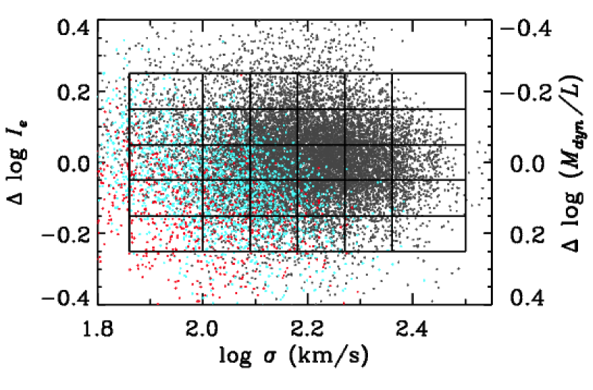
Figure 1.— Bins used to sort and stack “similar” galaxy spectra. The quantity $\Delta\log I_{e}$ is defined as the difference between the measured $\log I_{e}$ of each galaxy and the best-fitting FP relation (see Figure 1 of Paper II). Because $\Delta\log I_{e}$ is defined at fixed values of $\sigma$ and $R_{e}$, it is equivalent to $-\Delta\log(M_{dyn}/L_{V})$. Colors indicate the absolute magnitude range of the galaxies to give a sense of sample completeness. Dark gray points indicate galaxies with $M_{r}<-20.1$, for which our sample is volume-limited. Red points indicate the faint end of the sample ($M_{r}>-19.7$), where it is missing $\geq 50$% of the volume-limited targets. Cyan points indicate intermediate galaxies with $-20.1<M_{r}<-19.7$. Bins with low values of $\sigma$ and $\Delta\log I_{e}$ are substantially incomplete and are populated by galaxies from the low-redshift end of our sample ($0.04<z<0.05$).

2. Data

The galaxy sample used in this work is the same as that used in Papers I, II, and III. It consists of $\sim$16,000 early-type galaxies from the SDSS Main Galaxy Sample (Strauss et al. 2002) in the redshift range $0.04<z<0.08$. The early-type galaxy selection is described in detail in Paper I. Briefly, we require galaxies to have no significant detectable flux in the H$\alpha$ and [Oii]$\lambda$3727 emission lines (i.e., line fluxes are both below a $2\sigma$ detection threshold), to have concentrated light profiles (i.e., the ratio of the 90% and 50% Petrosian radii $R_{90}/R_{50}>2.5$ in the $i$-band), and to have light profiles that are better fit by a de Vaucouleurs profile than by an exponential profile. The resultant sample is strongly concentrated on the red sequence (see Figure 1 of Paper I). Spectra for the galaxies that meet these criteria are downloaded from the SDSS Data Archive Server. The various FP parameters are obtained from the SDSS Data Release 6 (DR6; Adelman-McCarthy et al. 2008) Catalog Archive Server (CAS) and the NYU Value-Added Catalog (Blanton et al. 2005) for Data Release 4 (DR4; Adelman-McCarthy et al. 2006), as described in Paper II. The individual galaxy spectra typically have signal-to-noise $S/N\sim 20$ Å^-1, so we sort the galaxies into bins based on their FP parameters, then stack the spectra within each bin to obtain very high $S/N$ mean spectra that span the binned parameter space.

In Paper II, we showed that the stellar population properties and therefore the star formation histories of early-type galaxies depend strongly on $\sigma$ and also on $\Delta I_{e}$ residuals at fixed $\sigma$ and fixed $R_{e}$. However, on the FP midplane all the stellar population properties investigated in Paper II showed no dependence on $R_{e}$. In this work we simplify the galaxy structural space by marginalizing over $R_{e}$, such that galaxy properties are defined in the 2D space of $\sigma$ and $\Delta I_{e}$ only.

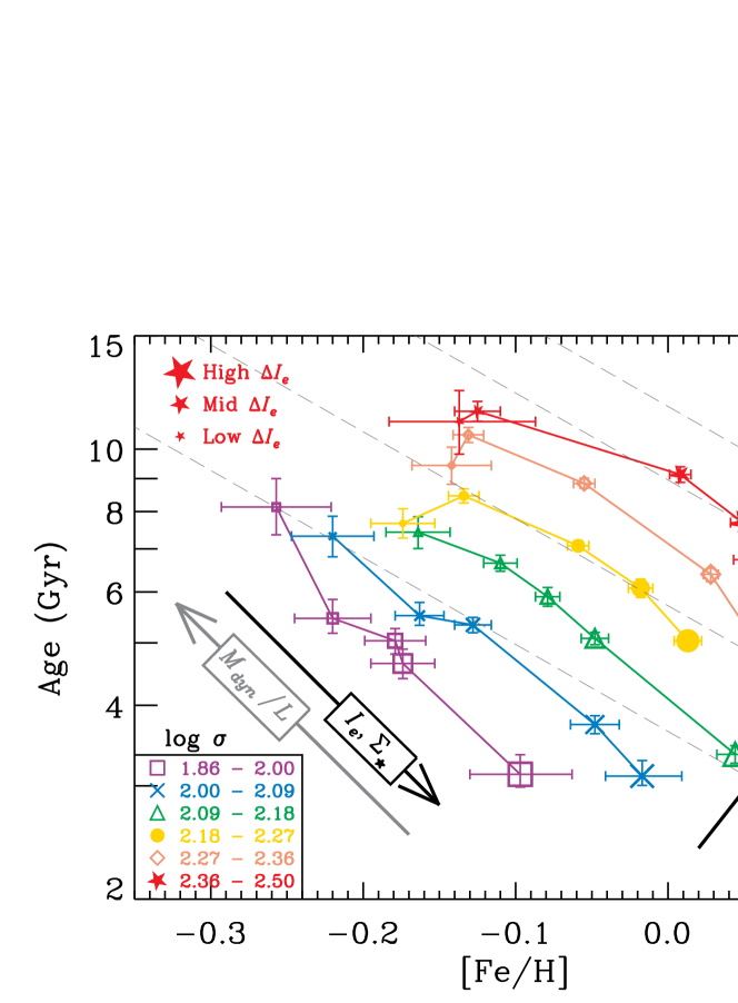
Figure 2.— The age-[Fe/H] hyperplane for early-type galaxies. Colors and symbols show different bins in $\sigma$, as indicated. Symbol size indicates bins in $\Delta I_{e}$ at intervals of 0.1 dex, with the smallest (largest) symbols indicating the lowest (highest) $\Delta I_{e}$ bins. Dashed lines are lines of constant $\sigma$ from the Trager et al. (2000a) metallicity hyperplane. On average, high-$\sigma$ galaxies have older ages and higher [Fe/H] than low-$\sigma$ galaxies. At fixed $\sigma$, age and [Fe/H] are anti-correlated and this relation is driven by $\Delta I_{e}$, with low (high) $\Delta I_{e}$ galaxies showing older (younger) ages and lower (higher) [Fe/H]. This anti-correlation between age and [Fe/H] may indicate that galaxies with low $\Delta I_{e}$ experienced shorter-duration star formation than their high $\Delta I_{e}$ counterparts at the same $\sigma$ (see text for details).

The FP for our galaxy sample is shown edge-on in Figure 1 of Paper II. Deviations from the plane are parameterized as $\Delta\log I_{e}$, where $\Delta\log I_{e}$ is defined as the difference between the measured value of $\log I_{e}$ for each galaxy and the fitted FP, such that

$$\Delta I_{e}\equiv\log(I_{e})-(1.16\log\sigma-1.21\log R_{e}+0.55).$$ (1)

Note that because $\Delta I_{e}$ is defined at fixed $\sigma$ and fixed $R_{e}$, there is a one-to-one equivalence (although a sign change) between $\Delta\log I_{e}$ and $-\Delta\log(M_{dyn}/L)$, since $M_{dyn}/L\propto\sigma^{2}R_{e}/I_{e}R_{e}^{2}\propto\sigma^{2}/I_{e}R_{e}$.

To group similar galaxies, we define a regular grid in $\Delta I_{e}$–$\sigma$ space as shown in Figure 1. The right-hand axis reflects the equivalence between $\Delta\log I_{e}$ and $-\Delta\log(M_{dyn}/L)$. Within each bin, we stack all galaxy spectra using a $\sigma$-clipping algorithm and rejecting color outliers, as described in Paper I. In each stacked spectrum, we measure the full set of Lick indices (Worthey et al. 1994; Worthey & Ottaviani 1997), along with estimated errors derived from the error spectra following the formalism of Cardiel et al. (1998). We model the mean luminosity-weighted SSP age, [Fe/H], [Mg/H] and [Mg/Fe], along with the statistical errors in each quantity, using the stellar population models of Schiavon (2007) and the EZ_Ages code developed by Graves & Schiavon (2008, see this work for details of the modeling process). The properties of the galaxies in each bin, the measured Lick index values, and the derived stellar population properties are given in Table 1.

As always, when interpreting SSP “age” measurements, one should bear in mind that the quoted age values are Balmer line strength-weighted, luminosity-weighted mean ages. For populations with extended star formation histories such as galaxies, the SSP ages are strongly biased toward the age of the youngest sub-populations of galaxies (e.g., Trager & Somerville 2009). Furthermore, the SSP ages presented in this paper are averaged over many similar galaxies. Thus, if one galaxy bin has a younger SSP age than another, this does not mean that all the stars in all of those galaxies are younger. Rather, it should be interpreted to mean that at least some (possibly quite small) fraction of the total star formation in those galaxies occurred up until more recently in the “younger” object than in the “older” one.

3. The 2D Family of Stellar Populations in Early-Type Galaxies

3.1. The Age-[Fe/H] Hyperplane

The first result of this paper is shown in Figure 2, which plots the age and [Fe/H] results from the stellar population analysis for the various bins in $\sigma$ and $\Delta I_{e}$. Colors and symbols give the $\sigma$ values for each bin of galaxies, as indicated in the figure key. Symbol sizes indicate bins in $\Delta I_{e}$, with the largest and smallest symbols representing the highest and lowest values of $\Delta I_{e}$, respectively. A version of this figure was presented in Paper III to demonstrate that galaxy star formation histories vary smoothly through FP space and to discuss $M_{\star}/L$ modeling. Here, we present a simplified form, which collapses all values of $R_{e}$ into a single point in order to show the main trends more clearly. The well-known trends of age and [Fe/H] with $\sigma$ are recovered: age and [Fe/H] both increase with increasing $\sigma$.

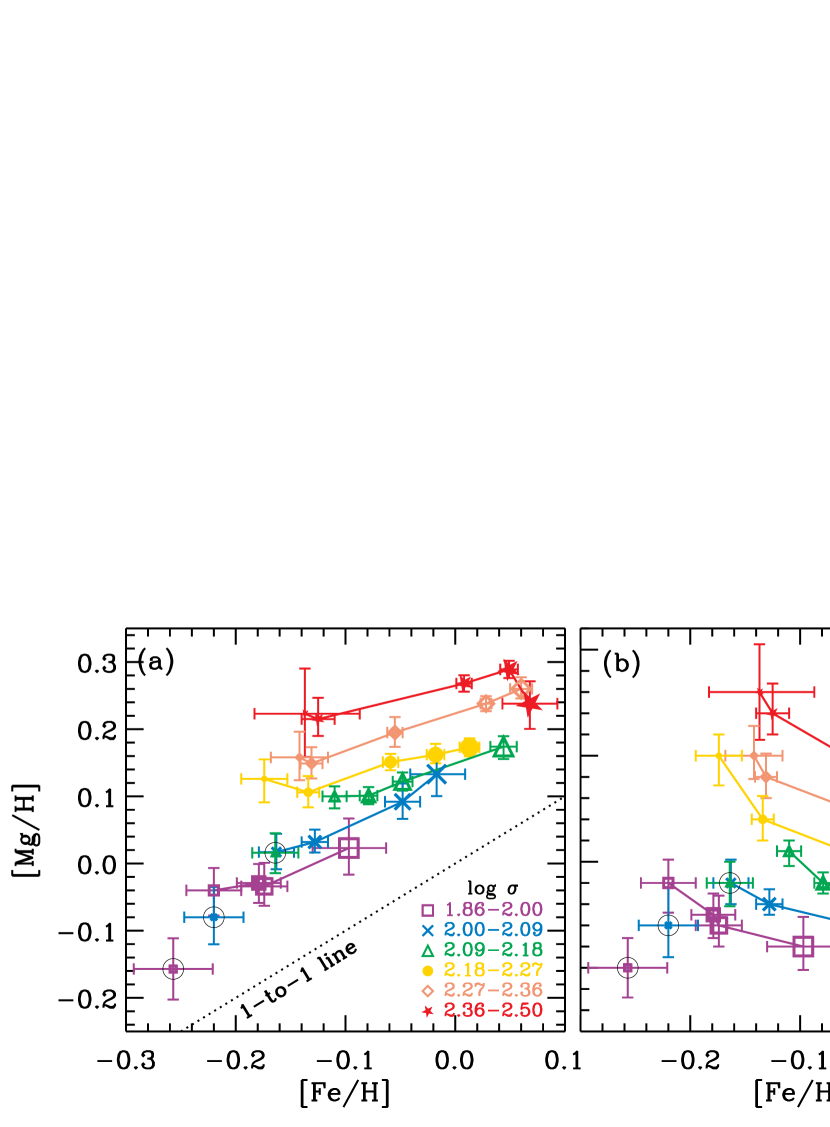
Figure 3.— (a) [Mg/H] as measured in the stacked spectra, shown as a function of [Fe/H]. As in Figure 2, colors and symbols show different bins in $\sigma$, while symbol size indicates bins in $\Delta I_{e}$. At fixed $\sigma$, both [Fe/H] and [Mg/H] increase with increasing $\Delta I_{e}$. The slope of the relation is shallower than one-to-one (dotted line), indicating that [Fe/H] varies more at fixed $\sigma$ than does [Mg/H]. [Mg/H] is always higher than [Fe/H], indicating that all galaxies have super-solar Mg/Fe ratios, with an offset that increases with $\sigma$. (b) The same plot for [Mg/Fe]. At fixed $\sigma$, [Fe/H] and [Mg/Fe] are anticorrelated with the strongest anticorrelation in the highest-$\sigma$ galaxies. Galaxies with low [Fe/H] span a range of [Mg/Fe], but all Fe-rich galaxies have relatively low values of [Mg/Fe]. The lowest $\Delta I_{e}$ bins for the three lowest values of $\sigma$ (outlined with black circles) deviate significantly from the [Mg/Fe] values expected from the rest of the data, and are discussed in detail in section 5.4

Furthermore, galaxies within a given $\sigma$ bin span a range in age and [Fe/H], with age and [Fe/H] anti-correlated at fixed $\sigma$ such that older galaxies have lower [Fe/H] than their younger counterparts at the same $\sigma$. This anti-correlation of age and [Fe/H] is essentially identical to the “metallicity hyperplane” of Trager et al. (2000a) except that our iso-$\sigma$ lines are slightly converging and curved, whereas those of Trager et al. (2000a) were straight and parallel (hence their term hyperplane). Lines of constant $\sigma$ from the Trager et al. Fe-hyperplane are overplotted as dashed lines. As expected, these run nearly parallel to our SDSS data for a given value of $\sigma$. There is a zeropoint offset between the Trager et al. (2000a) hyperplane and our iso-$\sigma$ lines due to zeropoint differences between the stellar population models used in the two analyses. With the updated models used in this analysis, we do not find galaxies with ages older than 12 Gyr, whereas the Trager et al. (2000a) sample contains galaxies with ages $>18$ Gyr.

An important result of this series of papers is that the anti-correlation of age and [Fe/H] at fixed $\sigma$ is driven by variations in $\Delta I_{e}$, or equivalently by variations in $\Delta\log(M_{dyn}/L)$. This was shown qualitatively in Paper II and will be quantified below. The correlation between galaxy star formation histories and structural properties is such that the oldest, most Fe-poor galaxies in a given $\sigma$ range are the galaxies with the lowest values of $\Delta I_{e}$, while the youngest, most Fe-rich galaxies are those with the highest values of $\Delta I_{e}$. Variations in $\Delta I_{e}$ are evidently associated with differences in star formation history between early-type galaxies with the same $\sigma$.

In Paper III, we demonstrated that stellar population $M_{\star}/L$ effects can only account for a small fraction of the variation in $I_{e}$ through the thickness of the FP. This means that variations in $I_{e}$ must be due primarily to variations in the effective stellar mass surface density in galaxies ($\Sigma_{\star}$), assuming that our constant-IMF and model stellar mass estimates are valid. Thus the oldest, most Fe-poor galaxies at a given value of $\sigma$ are those with the lowest $\Sigma_{\star}$.

The directions of increasing $\sigma$, $I_{e}$, $\Sigma_{\star}$, and $M_{dyn}/L$ are indicated on Figure 2 by black and gray arrows, as labelled. These arrows reveal that the 2D family of stellar population properties can be mapped onto a cross-section through the FP, with $\sigma$ along one axis and $\Delta I_{e}$ along the other. In other words, a galaxy’s location above or below the FP is related to how it formed stars, and the metallicity hyperplane shows how star formation history maps onto slices through FP space. This mapping is explored further in §3.3.

There have been some indications of this variation in previous work. As mentioned above, Forbes et al. (1998) and Terlevich & Forbes (2002) found that galaxy ages correlate with residuals from the FP, but in neither case do they identify or discuss the correlation of FP residuals with galaxy metallicities. Simultaneous with our Paper II, Gargiulo et al. (2009) reported similar results based on 141 early-type galaxies in the Shapley supercluster, which show that stellar population properties, and [Mg/Fe] in particular, correlate with residuals from the FP. Their observational results agree with the results of Paper II, although they parameterize FP residuals in terms of $R_{e}$ residuals at fixed $\sigma$ and fixed $I_{e}$ and therefore present the correlations differently.

3.2. Trends in Mg Enrichment

Like [Fe/H], [Mg/H] also shows variation with both $\sigma$ and with $\Delta I_{e}$ but the detailed behavior is different. Figure 3a shows [Mg/H] versus [Fe/H] for the various bins in $\sigma$ and $\Delta I_{e}$. Colors and symbols are as in Figure 2 and solid lines connect bins with the same $\sigma$. At fixed $\sigma$, [Fe/H] and [Mg/H] are correlated with a slope somewhat shallower than the one-to-one relation (shown as the dotted line for reference). The shallowness of the slope indicates that [Mg/H] changes less at fixed $\sigma$ than does [Fe/H].

The slope of the relation appears somewhat steeper for the lower three $\sigma$ bins than it does for the higher three $\sigma$ bins. However, this effect is almost entirely due to three data points: for the lower three $\sigma$ bins, the lowest $\Delta I_{e}$ points (outlined with black circles) have significantly lower values of [Mg/H] than would be expected from a simple extrapolation of the relation for the remaining $\Delta I_{e}$ bins at that $\sigma$. We return to these outliers below.

Galaxies at all values of $\sigma$ are offset vertically from the one-to-one relation (dotted line) such that [Mg/H] is always higher than [Fe/H]. This indicates that the galaxies in this sample have super-solar Mg enhancements. Futhermore, the size of the offset increases with increasing $\sigma$, indicating that the Mg enhancement scales with $\sigma$. This result is by now familiar (e.g., Kuntschner & Davies 1998, Jørgensen 1999, Trager et al. 2000a).

Another way to parameterize the Mg-enrichment process in galaxies is to compare Mg abundances with those of Fe by looking at [Mg/Fe]. This abundance ratio is not a new independent variable—it is in fact defined as [Mg/H]$-$[Fe/H]—but it is conceptually useful in the following discussion to examine Mg trends both in terms of [Mg/H] and [Mg/Fe]. In Figure 3b, we plot [Mg/Fe] as a function of [Fe/H] for the stacked spectra. Colors and symbols are as before. Galaxies appear to populate a wedge shape in this diagram, such that all galaxies with high values of [Mg/Fe] have relatively low values of [Fe/H], while galaxies with low [Mg/Fe] span a range in [Fe/H]. The galaxies with the highest values of [Mg/Fe] all have modest values of [Fe/H], suggesting that high Mg-enhancements come at the cost of high Fe production in chemical evolution.

Previous investigations of the “metallicity hyperplane” have not included [Mg/Fe] among the stellar population properties that vary at fixed $\sigma$ (e.g., Trager et al. 2000a; Smith et al. 2008a), while Thomas et al. (2005) quantify the intrinsic variation in [$\alpha$/Fe] at fixed $\sigma$ (they find $\Delta$[$\alpha$/Fe] $\approx$ 0.05 dex) but do not correlate this scatter with other galaxy observables. Thus the addition of [Mg/Fe] to the spread of the metallicity hyperplane at fixed $\sigma$ is new to this series of papers (see also the simultaneous work of Gargiulo et al. 2009).

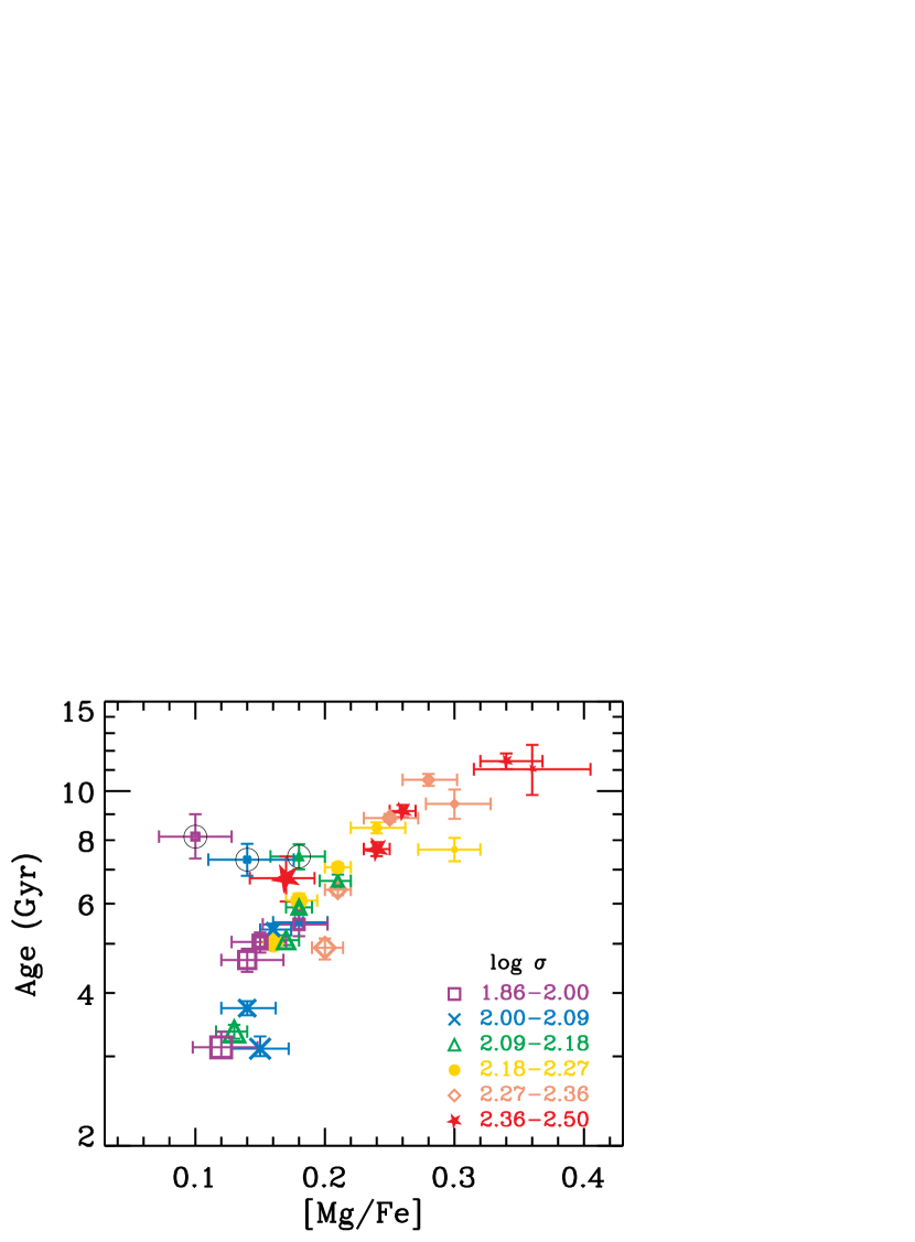
Figure 4.— Mean light-weighted age versus [Mg/Fe], as measured in the stacked spectra. Colors and symbols are as in Figures 2–3. The three outlying data points from Figure 3b stand out strongly (see section 5.4). Aside from these, SSP age and [Mg/Fe] are strongly correlated, with Mg-enhanced populations having the oldest ages.

In this space, the three outliers identified in Figure 3a stand out even more clearly. For the three lowest $\sigma$ bins, the lowest-$\Delta I_{e}$ galaxies (outlined with black circles) have unexpectedly low values of [Mg/Fe], which lie as much as 0.14 dex below the value one would derive from an extrapolation of the other data. It is worth noting that, while their values of [Mg/Fe] are unexpectedly low, their [Fe/H] values are a reasonable extrapolation of the higher-$\Delta I_{e}$ data at the same $\sigma$. This suggests that it is the Mg enrichment process, not that of Fe, that deviates in these galaxies. We return to this point in section 5.4.

Figure 4 plots the mean light-weighted ages against [Mg/Fe] for each of the stacked spectra. Colors and symbols are as in Figures 2–3. Ignoring the outlier data for the moment, there is a tight relation between age and [Mg/Fe], such that galaxies with the oldest stellar populations are the most strongly Mg enhanced. Keeping in mind that the observed SSP ages are biased toward young subpopulations, this means that galaxies with some quantity of more recent star formation (i.e., those with SSP ages $<6$ Gyr) all have relatively low levels of Mg enhancement ([Mg/Fe] $<0.2$). Galaxies with substantial Mg enhancements have uniformly old populations.

In this projection, the three outlying data points with surprisingly low [Mg/Fe] stand out very strongly: they do not follow the tight age-[Mg/Fe] relation of the other galaxies. The discrepancy varies systematically with $\sigma$, being largest for the lowest-$\sigma$ bin. All three points deviate in a consistent way, suggesting that this deviation is real. This means that any physical explanation for the strong age-[Mg/Fe] correlation must also explain why low-$\sigma$, low-$\Sigma_{\star}$ galaxies might deviate from it. We will return to these galaxies in section 5.4.

3.3. Mapping the Age-[Fe/H] Hyperplane onto a Cross-Section Through the FP

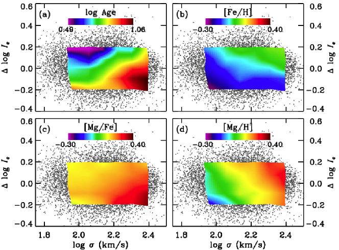
Figure 5.— Typical stellar population properties of early-type galaxies, mapped through $\sigma$–$\Delta I_{e}$ space. This space corresponds to a cross-section through the FP. Gray points show the values of $\sigma$ and $\Delta I_{e}$ for individual galaxies in the sample. The overlaid color contours show the results of our stellar population analysis of the stacked spectra. Age, [Fe/H], [Mg/H], and [Mg/Fe] all increase with $\sigma$. At fixed $\sigma$, age and [Mg/Fe] decrease with increasing $\Delta I_{e}$, while [Fe/H] and [Mg/H] increase with increasing $\Delta I_{e}$.

It is clear from Figures 2–4 that the stellar population properties of early-type galaxies depend on both $\sigma$ and $\Delta I_{e}$ in systematic ways. The correspondence between the structural properties of galaxies and their stellar populations can be represented by mapping age, [Fe/H], [Mg/H], and [Mg/Fe] onto $\sigma$–$\Delta I_{e}$ space. This mapping is shown in Figure 5. As defined, $\sigma$–$\Delta I_{e}$ space corresponds to a cross-section projected through the FP (i.e., marginalizing over $R_{e}$). In each panel of Figure 5, gray points indicate the location of the sample galaxies in $\sigma$–$\Delta I_{e}$ space, analogous to Figure 1. The data have been overlaid with color contours representing the typical values of each stellar population parameter at that location. These color contours are computed by plotting the derived stellar population parameter values for each stacked spectrum at the point corresponding to the mean values of $\sigma$ and $\Delta I_{e}$ for that galaxy bin. We then interpolate between the $6\times 5$ grid of values from the stacked spectra to map the stellar population parameters across the space.

Shown this way, mean luminosity-weighted age (panel a) and [Mg/Fe] (panel c) track one another fairly closely, as expected from Figure 4, with lines of constant age and lines of constant [Mg/Fe] running diagonally from lower left to upper right in the maps. This means that both age and [Mg/Fe] have their lowest values for low-$\sigma$, high-$\Delta I_{e}$ galaxies and their maximum values for high-$\sigma$, low-$\Delta I_{e}$ galaxies.

In contrast, lines of constant [Fe/H] and lines of constant [Mg/H] run diagonally from upper left to lower right, so that [Fe/H] and [Mg/H] have their lowest values in low-$\sigma$, low-$\Delta I_{e}$ galaxies, and their maximum values in high-$\sigma$, high-$\Delta I_{e}$ galaxies. This is another illustration that the family of early-type galaxy stellar population properties is inherently two-dimensional and further that Fe does not behave like Mg.

Although there is broad agreement in the behavior of age and [Mg/Fe] and also in the behavior of [Fe/H] and [Mg/H], the trends are different in detail. The rough correspondence in the behavior of age and [Mg/Fe] breaks down at low $\sigma$, where [Mg/Fe] becomes nearly constant for all galaxies. This is expected from Figure 4, which shows a steepening of the age–[Mg/Fe] relation such that [Mg/Fe] $\sim 0.15$ for a substantial range of ages. As for the differences between [Fe/H] and [Mg/H], the contours have different slopes, such that [Fe/H] shows more variation with $\Delta I_{e}$ than does [Mg/H].

4. Quantifying Stellar Population and Mass-to-Light Variations in FP Space

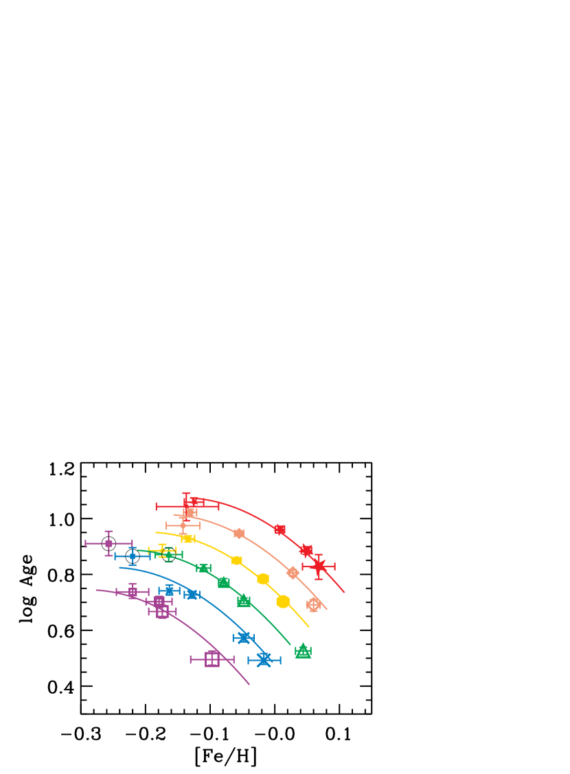
Figure 6.— Comparing the functional fits to the observed data in age-[Fe/H] hyperspace. The data are as in Figure 2. The solid lines show the fits from equations 2 and 3, color-coded to match the corresponding $\sigma$ bins. Including a quadratic $(\Delta I_{e})^{2}$ term in the age fit produces curvature that closely matches that in the observed galaxies. Note that the lowest-$\Delta I_{e}$ galaxies in the lower two $\sigma$ bins have ages substantially older than those predicted by the fits. These are the same galaxies that show unexpectedly low values of [Mg/Fe] in Figure 3b (see section 5.4 for details).

4.1. Galaxy Properties in 2D: as Functions of $\sigma$ and $\Delta I_{e}$

The consistent behavior of the various stellar population properties throughout these FP cross-sections makes it possible to write each property as a function of $\sigma$ and $\Delta I_{e}$. We use the IDL package mpfit.pro (Markwardt 2009) to fit robust non-linear least squares curves in multiple dimensions, taking into account variable error bars. A good fit for age as a function of $\sigma$ and $\Delta I_{e}$ requires some curvature (as suggested by Figure 2), which we include as a quadratic term in $\Delta I_{e}$. The resulting age relation is

$$\begin{split}\log age=&\phantom{(}0.82+\phantom{(}0.75\phantom{.}\log\sigma^{\prime}-0.85\phantom{.}\Delta I_{e}-1.9\phantom{.}(\Delta I_{e})^{2}\\ &(0.01)\phantom{+}(0.02)\phantom{\log\sigma^{\prime}-}(0.03)\phantom{\Delta I_{e}-}(0.2),\end{split}$$ (2)

where $\sigma^{\prime}=\sigma/150$ km s^-1 and $\Delta I_{e}\equiv\log I_{e}-(1.16\log\sigma-1.21\log R_{e}+0.55)$, as defined in Equation 1. The numbers in parentheses give the 1$\sigma$ errors on the quoted parameters, based on the uncertainties in the measured stellar population parameters (see the values in Table 1 and error bars in Figures 2-3).

[Fe/H], [Mg/H], and [Mg/Fe] can all be fit well with simple planar relations, which give

$$\begin{split}\mbox{[Fe/H]}=&-0.08+\phantom{(}0.33\phantom{.}\log\sigma^{\prime}+0.59\phantom{.}\Delta I_{e}\\ &\phantom{-}(0.01)\phantom{+}(0.02)\phantom{\log\sigma^{\prime}-}(0.02),\end{split}$$ (3)

$$\begin{split}\mbox{[Mg/H]}=&\phantom{(}0.12+\phantom{(}0.66\phantom{.}\log\sigma^{\prime}+0.30\phantom{.}\Delta I_{e}\\ &(0.01)\phantom{+}(0.03)\phantom{\log\sigma^{\prime}+}(0.04),\end{split}$$ (4)

and

$$\begin{split}\mbox{[Mg/Fe]}=&\phantom{(}0.20+\phantom{(}0.28\phantom{.}\log\sigma^{\prime}-0.29\phantom{.}\Delta I_{e}.\\ &(0.01)\phantom{+}(0.02)\phantom{\log\sigma^{\prime}-}(0.03),\end{split}$$ (5)

respectively. For [Mg/Fe], the three outlying data points (see section 3.2) were not included in the fit.

Figure 6 provides a visual confirmation of the quality of these fits by comparing the age and [Fe/H] fits to the observed values. The data, shapes, and color-coding are as in Figure 2. For each $\sigma$ bin, we compute a curve from the age and [Fe/H] fits given in equations 2 and 3. The curve for each bin is computed with $\sigma$ fixed to the mean value for that bin ($\log\sigma=1.95$, 2.05, 2.14, 2.22, 2.31, and 2.39 for the six bins, respectively) and for a range of $\Delta I_{e}$, with $-0.2<\Delta\log I_{e}<0.2$. These are overplotted as solid lines, with colors corresponding to the $\sigma$ bins represented.

The fits do an excellent job of reproducing the data, with the exception of two points: the lowest-$\Delta I_{e}$ bins for the two lower $\sigma$ bins. In these bins, the observed stellar population ages are significantly older than expected from the fits. These are the same data that show discrepant values of [Mg/Fe] in Figure 3. They will be discussed in detail in section 5.4.

The quality of the fits is quantified in Figure 7. In each panel, the x-axis shows the values predicted by Equations 2–5 based on the mean values of $\sigma$ and $\Delta I_{e}$ for each galaxy bin, while the y-axis shows the stellar population parameters as measured in the stacked spectra. Colors and symbols are as in Figures 2–4. When the stellar population parameters are fit as functions of both $\sigma$ and $\Delta I_{e}$, the resulting relations are much tighter than would be derived from fitting just $\sigma$, as can be seen by the substantial spread in values at fixed $\sigma$.

In each panel, the inset histogram shows the distribution of offsets from the planar fits expressed in units of the $1\sigma$ measurement errors for each data point (i.e., the quantity offset/error). These can be compared to a gaussian distribution centered at zero with $\sigma=1$ (overplotted lines). For [Mg/Fe] and [Mg/H], the fits in equations 4–5 replicate the observations within the observational errors. The fits to age and [Fe/H] are not quite as good but still indicate that the fitting functions given in equations 2 and 3 are a reasonable representation of the data.

Overall, the good agreement between the data and the fits illustrates that the fitting functions give a good representation of the typical stellar population properties for early-type galaxies as functions of $\sigma$ and $\Delta I_{e}$. They provide a new tool for estimating the stellar population properties of early-type quiescent galaxies for which values of $\sigma$, $R_{e}$, and $L$ can be measured but for which high-quality spectra are not available.

4.2. Galaxy Properties in 3D: as Functions of $\sigma$, $R_{e}$, and $\Delta I_{e}$

This paper focuses on stellar population variations in the 2D projected cross-section through the FP. We have justified dropping the third FP dimension, $R_{e}$, because Paper II showed that the stellar population properties of our quiescent galaxy sample are independent of $R_{e}$ at fixed $\sigma$. It is however instructive to return to 3D FP space briefly, which we do in this section, in order to verify (and quantify) the lack of stellar population variation with $R_{e}$. Furthermore, the various mass-to-light ratios, stellar masses, and stellar mass surface densities of our sample galaxies do depend on $R_{e}$, and we need to be in 3D space to model these additional quantities.

To do this, we bin the galaxies in a 3D parameter space defined by $\sigma$, $R_{e}$, and $\Delta I_{e}$. This binning system is described in detail in Paper II, in which we determine the mean SSP age, [Fe/H], [Mg/H], and [Mg/Fe] for each bin of galaxies in the 3D space. In Paper III, we further measure dynamical and stellar masses ($M_{dyn}$ and $M_{\star,IMF}$), as well as mass-to-light ratios and stellar mass surface densities using this system.

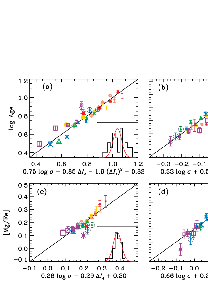
Figure 7.— Residuals from fits to the stellar population age, [Fe/H], [Mg/H], and [Mg/Fe] as functions of $\sigma$ and $\Delta I_{e}$. In each panel, the x-axis gives the stellar population parameter value as predicted by Equations 2–5, based on the average value of $\sigma$ and $\Delta I_{e}$ in each bin of galaxies. The values predicted by the fits are compared to the actual values measured from the stacked spectra on the y-axis. Solid lines show one-to-one relations. Colors and symbols represent $\sigma$ and $\Delta I_{e}$ bins, as in Figures 2–4. The outliers are circled in black. The insets show the distribution of offsets from the fits (black histogram) in units of the $1\sigma$ measurement errors, compared to a gaussian distribution with $\mu=0$ and $\sigma=1$ (over-plotted line). The insets demonstrate that Equations 2–5 predict [Mg/H] and [Mg/Fe] within the observational errors, but that the difference between predicted and observed values for age and [Fe/H] show slightly more scatter than can be accounted for by the observational errors. See text for details.

Here, we fit each of the stellar population parameters ($\log age$, [Fe/H], [Mg/H], and [Mg/Fe]) as functions of $\sigma$, $R_{e}$, and $\Delta I_{e}$. The procedure is similar to that in the previous section except that here we are fitting in four dimensions instead of three. Again, we restrict all fits to be first order in each parameter with the exception of age, which we allow to include a quadratic term in $\Delta I_{e}$. These fits are summarized in the first section of Table 2, labelled “stellar populations.” The quoted errors include only the formal uncertainties in the fits as estimated by mpfit.pro. Presented in this way, the $\log\sigma$ column of the table indicates how much the parameter in each row (e.g., $\log age$ or [Fe/H]) changes for each 1.0 dex change in $\sigma$. It also means that each row can be converted into a functional form. For example, the first row of the table can be rewritten as an equation for $\log age$, such that

$$\begin{split}\log age=0.85+0.73\log\sigma^{\prime}+0.02\log R_{e}^{\prime}\\ -0.92\Delta I_{e}-2.9(\Delta I_{e})^{2},\end{split}$$ (6)

where $R_{e}^{\prime}=R_{e}/2.5$ kpc.

The second section of Table 2 (labelled “mass-to-light ratios”) gives the parameters of fits for the dynamical mass-to-light ratio ($M_{dyn}/L$), the component of $M_{dyn}/L$ contributed by dark matter or IMF variations ($M_{dyn}/M_{\star,IMF}$), and the component of $M_{dyn}/L$ contributed by stellar population variations ($M_{\star,IMF}/L$). The third section (labelled “stellar mass”) also includes the stellar mass ($M_{\star,IMF}$) and stellar surface mass density within $R_{e}$ ($\Sigma_{\star,IMF}$). The fits in these two sections are taken from Table 2 of Paper III, except for the $M_{\star}$ fits, which are newly computed here in an identical manner to the other fits. In all cases, the “IMF” subscript indicates a stellar mass or stellar surface mass density that has been computed assuming a Chabrier IMF. The effect of variable IMFs, if any, would be included in the $M_{dyn}/M_{\star,IMF}$ term (see Paper III for a thorough discussion of this point).

Notice that all four stellar population parameters are essentially independent of $R_{e}$ in that they show 0.04 dex or less variation per dex of variation in $R_{e}$. The data span almost a full dex in $R_{e}$, but no systematic trends in stellar population age, [Fe/H], [Mg/H], or [Mg/Fe] are observed. Meanwhile, all four parameters depend strongly on both $\sigma$ and $\Delta I_{e}$, with values similar to those from the 2D fits of section 4.1. The differences between the 3D values in Table 2 and the 2D values in equations 2–5 are in all cases consistent with the errors quoted for the fits.

Table 23D Fits: Stellar Pops and Mass Parameters as Functions of $\sigma$, $R_{e}$, and $\Delta I_{e}$

	Zeropoint		$\log\sigma$		$\log R_{e}$		$\Delta I_{e}$		$(\Delta I_{e})^{2}$
Range Covered by Data			0.5 dex		0.9 dex		0.4 dex
Stellar Populations
$\log age$	$0.85$ $\pm$	0.01	$0.73$ $\pm$	0.05	$0.02$ $\pm$	0.03	$-0.92$ $\pm$	0.07	$-2.9$ $\pm$	0.5
[Fe/H]	-0.09 $\pm$	0.01	$0.27$ $\pm$	0.04	$0.04$ $\pm$	0.02	$0.64$ $\pm$	0.04	… $\pm$	…
[Mg/H]	0.11 $\pm$	0.01	$0.58$ $\pm$	0.04	$0.02$ $\pm$	0.04	$0.35$ $\pm$	0.05	… $\pm$	…
[Mg/Fe]	0.20 $\pm$	0.01	$0.27$ $\pm$	0.03	$-0.005$ $\pm$	0.02	$-0.27$ $\pm$	0.04	… $\pm$	…
Mass-to-Light Ratios
$\log\phantom{.}(M_{dyn}/L)$	0.62 $\pm$	0.01	$0.85$ $\pm$	0.01	$0.22$ $\pm$	0.01	$-1.04$ $\pm$	0.01	… $\pm$	…
$\log\phantom{.}(M_{dyn}/M_{\star,IMF})$	0.20 $\pm$	0.01	$0.53$ $\pm$	0.02	$0.22$ $\pm$	0.01	$-0.80$ $\pm$	0.02	… $\pm$	…
$\log\phantom{.}(M_{\star,IMF}/L)$	0.42 $\pm$	0.01	$0.31$ $\pm$	0.01	$0.003$ $\pm$	0.01	$-0.24$ $\pm$	0.02	… $\pm$	…
Stellar Mass
$\log M_{\star,IMF}$	10.6 $\pm$	0.01	$1.49$ $\pm$	0.02	$0.80$ $\pm$	0.01	$0.81$ $\pm$	0.02	… $\pm$	…
$\log\Sigma_{\star,IMF}$	3.81 $\pm$	0.01	$1.49$ $\pm$	0.01	$-1.20$ $\pm$	0.01	$0.80$ $\pm$	0.02	… $\pm$	…

Note. — $\sigma^{\prime}\equiv\sigma/150$ km s^-1 and $R_{e}^{\prime}\equiv R_{e}/2.5$ kpc. The units of $I_{e}$ are $L_{\odot}$ pc ^-2. All $L$ values are $V$-band luminosities. The “$IMF$” subscript on values of $M_{\star}$ and $\Sigma_{\star}$ indicates that they are computed assuming a Chabrier IMF. Any variation in the IMF would be contained within the $M_{dyn}/M_{\star,IMF}$ term. See Paper III for details.

*Correcting these values for differences in the fraction of the galaxy sampled by the SDSS $3^{\prime\prime}$ fiber gives the values $-0.06$ and $-0.08$ for [Fe/H] and [Mg/H], respectively, based on the radial metallicity gradients assumed by Smith et al. (2009). See text for details.

Smith et al. (2009) have suggested that aperture effects may affect observed trends with $L$ or $R_{e}$. The SDSS spectra are obtained using spectral fibers with diameters of $3^{\prime\prime}$; the fraction of the light sampled in each galaxy therefore depends on the galaxy’s size and distance. If the stellar populations in each galaxy have substantial radial gradients, these could create spurious (or mask real) stellar population trends with $R_{e}$. Adopting their suggested metallicity gradients (see section 2.6 of that work) and applying them to our observed values of [Fe/H] and [Mg/H], we find that the fits in Table 2 change modestly, such that the $R_{e}$ parameters for [Fe/H] and [Mg/H] become $-0.06$ and $-0.08$, respectively (as compared to their uncorrected values of $0.04$ and $0.02$). The $\sigma$ and $\Delta I_{e}$ parameter differences are within the quoted errors. These aperture-corrected values still show very weak dependence on $R_{e}$, indicating the the stellar population properties of quiescent galaxies are essentially independent of galaxy sizes.

As expected from the lack of stellar population variation with $R_{e}$, the stellar population component of the mass-to-light variation, $M_{\star,IMF}/L$, also shows no dependence on $R_{e}$. However, the dark matter (and/or IMF term) does depend on $R_{e}$, as do $M_{\star,IMF}$ and $\Sigma_{\star,IMF}$. Along the FP, the masses and mass distributions of galaxies depend on $R_{e}$ but their star formation histories do not.

Table 2 illustrates several other interesting points. It shows the expected inverse relationship between $\Delta I_{e}$ and $M_{dyn}/L$ at fixed ($\sigma$, $R_{e}$) in that $M_{dyn}/L$ changes by $-1.0$ dex for every one dex change in $\Delta I_{e}$. Moreover, $\sim$80% of the change in $\Delta I_{e}$ is due to variations in the IMF/dark matter component of the galaxy ($M_{dyn}/M_{\star,IMF}$), with only $\sim$20% due to stellar population variations ($M_{\star,IMF}/L$). This is discussed in detail in Paper III.

This dominance of $M_{dyn}/M_{\star,IMF}$ over $M_{\star,IMF}/L$ has a further implication: most of the change in $\Delta I_{e}$ is due to a real change in stellar surface density, $\Sigma_{\star,IMF}$. This is also evident from Table 2, which shows that $\Sigma_{\star,IMF}$ changes by $\sim$0.8 dex for every 1.0 dex change in $\Delta I_{e}$. Thus the observed $\Delta I_{e}$ variations about the FP are predominantly due to differences in the surface mass density of stars within $R_{e}$, not to stellar population mass-to-light ratio effects. It is therefore not possible for galaxies to evolve through the FP simply by fading—their stellar mass densities are ab initio different. We return to this key point in section 5.2.

4.3. Parameterizing FP Residuals in Terms of $R_{e}$ versus $I_{e}$

Concurrently with our Paper II, Gargiulo et al. (2009) published a study of stellar populations in 3D FP space based on a sample of 141 galaxies in the Shapley Supercluster. In that work, they parameterize residuals from the FP in terms of $R_{e}$ rather than $I_{e}$. As in Paper II, they find that residuals from the FP correlate with stellar population ages and [Mg/Fe]. The choice of $R_{e}$ as the dependent parameter is based upon the fact that the FP was originally proposed as a tool for measuring distances to galaxies, and therefore the distance-dependent quantity $R_{e}$ was historically fit as the free parameter against the distance-independent quantities $\sigma$ and $I_{e}$.

We prefer to parameterize residuals from the FP in terms of $I_{e}$ for two reasons. The first is that comparing galaxies at fixed values of $\sigma$ and $R_{e}$ means that they also have the same total dynamical masses, since $M_{dyn}\propto\sigma^{2}R_{e}$. More importantly, along the FP midplane the stellar populations of galaxies are observed to be independent of $R_{e}$. This is true over almost one dex of variation in $R_{e}$, which represents a much larger range of variation than the limited thickness of the FP. For understanding stellar populations, it is therefore logical to treat $R_{e}$ as an “inert” variable in the stellar population modelling and to parameterize the residuals of the FP and their correlated stellar population variations in terms of $I_{e}$. Of course, for distance studies using $R_{e}$, it is appropriate and necessary to set $R_{e}$ as the dependent variable.

5. The Star Formation Histories of Early-Type Galaxies

Having fully quantified the mapping between early-type galaxy structure and stellar populations, let us examine the trends illustrated in Figures 2–5 in greater detail. The goal is to interpret the observed variations in stellar population properties as differences in the star formation histories of the galaxies.

In the following discussion, we will differentiate between two effects that can modify the abundance patterns of galaxies. The first is the effective yield of metals during star formation, due to the chemical enrichment of the interstellar medium (ISM) by supernovae. Variations in effective yield also include differences in the relative effective yields of different elements, e.g., the Fe-peak elements predominantly produced by type Ia supernovae (SNe Ia) versus the $\alpha$-elements predominantly produced by type II supernovae (SNe II). The effective yield depends on the IMF, such that top-heavy IMFs with larger fractions of massive stars produce higher effective yields overall, as well as higher [$\alpha$/Fe] ratios. The effective yield also depends on gas inflow and outflow during star formation; closed box models for star formation produce different effective yields than those with substantial outflows of enriched material or inflows of primordial-abundance gas. In addition, the effective yield of SNe Ia elements (e.g., Fe) that is incorporated into stars (and hence is measured by absorption line studies) depends on the time-scale for star formation, as discussed below.

A second quantity with relevance for galaxy stellar abundance patterns is the baryon “conversion efficiency” of star formation, which measures the fraction of gas in a galaxy that is ultimately turned into stars. Galaxies with higher conversion efficiencies turn a larger fraction of their baryons into stars than those with lower conversion efficiencies. All other things being equal, this additional processing of baryonic material results in the production of more heavy elements over the star-forming lifetime of the galaxy and should result in higher abundances for all metals.

5.1. $\sigma$-Dependent Variations in Star Formation History

The various stellar population trends with $\sigma$ have been known for some time and their implications discussed by many authors. We briefly review some of this discussion here before moving on in section 5.2 to focus on the new results of this work: the variations at fixed $\sigma$.

As mentioned above, the effective yield of certain elements may depend upon the timescale for star formation. Short timescales for star formation are often discussed in the literature as a possible mechanism for producing low-[Fe/H], high-[Mg/Fe] galaxies due to the time-delay between the production of Mg (and other $\alpha$-elements) by SNe II and the slower production of Fe by SNe Ia (Tinsley 1979; Greggio & Renzini 1983). Numerous previous authors (e.g., Worthey et al. 1992; Matteucci 1994; Trager et al. 2000a; Thomas et al. 2005) have suggested that the duration of star formation ($\Delta t_{SF}$) may be shorter for more massive galaxies, resulting in an increase in [Mg/Fe] with increasing $\sigma$. Shorter duration star formation should result in fewer Fe-peak elements being incorporated into new generations of stars. This leads to lower levels of Fe relative to Mg and therefore to higher [Mg/Fe]. Thomas et al. (2005) have quantified this using a simple closed-box chemical evolution model to estimate a quantitative relationship between [$\alpha$/Fe] and $\Delta t_{SF}$ based on the chemical evolution models of Thomas et al. (1999).

All other galaxy properties being equal, this model for effective yield variations predicts higher [Mg/Fe] and lower [Fe/H] for galaxies with shorter $\Delta t_{SF}$. The predicted trend—an anti-correlation between [Fe/H] and [Mg/Fe]—is observed at fixed $\sigma$ in Figure 3. However, both [Fe/H] and [Mg/Fe] are observed to increase with increasing $\sigma$. This suggests that another effect must also be at work along the $\sigma$-sequence, a different mechanism that modifies the overall effective yield or changes the conversion efficiency of star formation versus $\sigma$.

One oft-cited possibility for this second mechanism involves relaxing the assumption of a closed-box model to include substantial quantitites of supernova feedback. Galaxies with lower values of $\sigma$ have shallower gravitational potential wells and are therefore more susceptible to SN feedback, limiting the chemical enrichment of the interstellar medium by SNe (e.g., Larson 1974; Arimoto & Yoshii 1987; Matteucci 1994; Pipino & Matteucci 2004). This process lowers the effective yield and tends to produce lower metallicities in lower-$\sigma$ galaxies. It should therefore result in lower values of both [Mg/H] and [Fe/H], as seen in galaxies with low $\sigma$.

If both of these processes vary with $\sigma$ such that higher-$\sigma$ galaxies have short $\Delta t_{SF}$ and are less affected by SN feedback, it is possible to explain the observed trends in [Fe/H], [Mg/H], and [Mg/Fe] with $\sigma$. Changing $\Delta t_{SF}$ with $\sigma$ can also produced the observed trends in age (e.g., Thomas et al. 2005), as galaxies which shut down star formation earlier will have older SSP ages. This dual picture—overall modulation by $\sigma$ and variation in $\Delta t_{SF}$ at fixed $\sigma$—is used to construct a semi-quantitative model in the next section.

5.2. A Toy Model for Galaxy Star Formation Histories

The galaxy data presented in this work also show variations in SSP age, [Fe/H], [Mg/H], and [Mg/Fe] in a second dimension that correlates with $\Delta I_{e}$ at fixed $\sigma$ (e.g., Figure 5). We hypothesize that, in addition to the proposed variations in $\Delta t_{SF}$ and SN feedback strength as a function of $\sigma$, there are variations in $\Delta t_{SF}$ in early-type galaxy progenitors at fixed $\sigma$.

This scenario is illustrated in Figure 8 by a set of toy models. This is a concrete and semi-quantitative representation of the model we first proposed in Paper III. In this schematic representation, star formation is approximated by top-hat models with constant star formation rates, i.e., star formation is “on” where indicated, and “off” everywhere else. In this simple formulation, galaxy star formation histories can be represented by two numbers: the duration of star formation ($\Delta t_{SF}$) and the onset time at which star formation begins ($t_{on}$). In the figure, typical galaxy star formation histories are grouped vertically as a function of $\sigma$, with color-coding as in Figures 2-4. The fill pattern indicates bins in $\Delta I_{e}$, as shown in the figure key. The three outlying data bins (see section 3.2) are excluded from the figure.

The duration of star formation is estimated for each bin by converting the value of [Mg/Fe] predicted by equation 5 into an estimate for $\Delta t_{SF}$. The conversion uses equation 4 from Thomas et al. (2005) ([$\alpha$/Fe] $\approx 1/5-1/6$ log $\Delta t_{SF}$). We substitute [Mg/Fe] for [$\alpha$/Fe] on the assumption that Mg enrichment traces the group of $\alpha$ elements as a whole. The Thomas et al. conversion from [Mg/Fe] to $\Delta t_{SF}$ is based on a closed-box chemical evolution model where star formation histories are assumed to have a gaussian shape with FWHM $=\Delta t_{SF}$. The simplified “on/off” representation in Figure 8 can be thought of as showing the FWHM peak of star formation in a gaussian model.

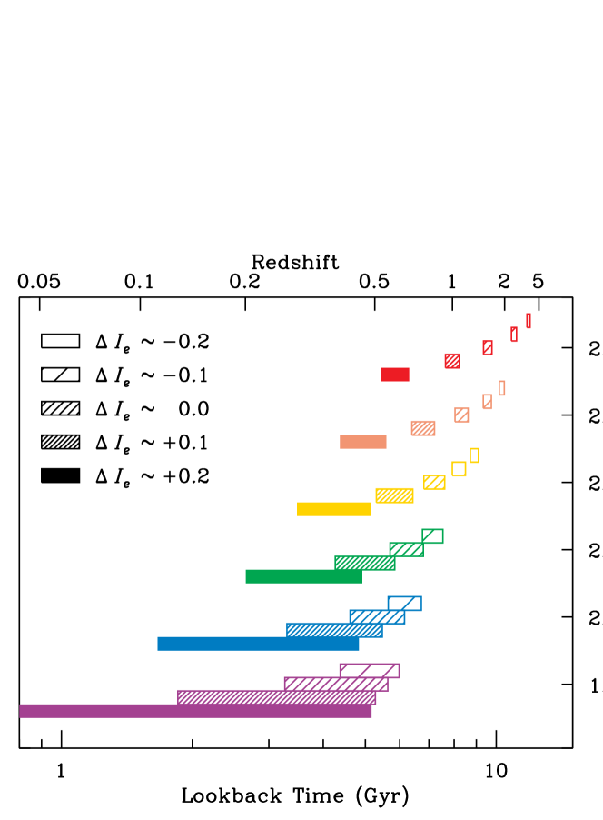
Figure 8.— Toy models for the star formation histories of early-type galaxies, based on the age and [Mg/Fe] fits given in equations 2 and 5 (see text for details). Different bins in $\sigma$ are color-coded as in previous figures. The three outlying data bins (see section 3.2) are excluded from the figure. Galaxies with low $\sigma$ typically begin star formation at later times and form stars over longer timescales than galaxies with higher $\sigma$. At fixed $\sigma$, the duration of star formation varies, with the highest-$\Delta I_{e}$ galaxies (filled bars) experiencing the most extended star formation and the lowest-$\Delta I_{e}$ galaxies (empty bars) experiencing the shortest duration of star formation. The range in $\Delta t_{SF}$ at fixed $\sigma$ leads to differing mean stellar ages and differing enrichment in SN Ia products that are in qualitative agreement with the trends shown in Figure 5.

The resulting epoch of star formation is centered on the mean age predicted for each bin by equation 2. Since $\Delta t_{SF}$ has already been fixed by the value of [Mg/Fe] for each bin, this effectively sets the value of $t_{on}$. Of course, these values are SSP ages rather than a true mass-weighted age. This means that the ages as represented in Figure 8 are skewed toward young values and later $t_{on}$ than is probably realistic. However, the goal is not to produce fully realistic, self-consistent star formation histories but rather to examine trends for how star formation histories vary between galaxies with different properties.

If we focus momentarily on “typical” galaxies that lie on the FP midplane (i.e., have $\Delta I_{e}\sim 0.0$), Figure 8 is qualitatively consistent with Figure 10 of Thomas et al. (2005). Galaxies with higher values of $\sigma$ form stars over shorter lengths of time and do the bulk of their star formation at higher redshift than lower-$\sigma$ galaxies. They follow “staged onset” star formation, in which galaxies with lower values of $\sigma$ have later $t_{on}$—they begin forming stars at later times (e.g., Noeske et al. 2007). They also manifest “downsizing” (Cowie et al. 1999) such that lower-$\sigma$ galaxies continue forming stars to later times than higher-$\sigma$ galaxies.

The main modification proposed here is the additional variation in $\Delta t_{SF}$ at fixed $\sigma$, such that galaxies with low $\Delta I_{e}$ have shorter duration star formation than those with high $\Delta I_{e}$. In its simplest form, this model would assume that all galaxies with the same $\sigma$ form the same total $M_{\star}$ but over different amounts of time (the “fixed total $M_{\star}$” model). This changes the effective yield of Fe, and thus the abundance patterns of galaxies with the same $\sigma$. The galaxies with different $\Delta I_{e}$ values at fixed $\sigma$ also have slightly different values of $t_{on}$ such that lower-$\Delta I_{e}$ galaxies start forming stars sooner than those with high-$\Delta I_{e}$. However, this result depends critically on the quantification of $\Delta t_{SF}$.

Table 3Trends in the Toy Models

Model	$\Sigma_{\star}$	[Mg/H]	[Mg/Fe]	[Fe/H]	Age
Fixed Total $M_{\star}$ Model	None	None	$+$	$-$	$+$
Premature Truncation Model	$-$	$-$	$+$	$-$	$+$
Observations	$-$	$-$	$+$	$-$	$+$

Note. — Trends give the sign of the effect toward lower $\Delta I_{e}$.

In general, we caution the reader against drawing strong quantitative conclusions from this simple toy model, for several reasons. Firstly, the quantification of $\Delta t_{SF}$ cannot be correct in detail, as can be seen by the fact that solar-scale abundances of [Mg/Fe] imply $\Delta t_{SF}>15$ Gyr in the prescription of Thomas et al. (2005). Secondly, the SSP values for the stellar population parameters are skewed from the true mass-weighted values. This is likely to have a substantial effect on the stellar ages and a weak effect on the inferred metallicities and abundance ratios (Trager & Somerville 2009). Thus the toy model presented in Figure 8 should be treated as an illustration of the inferred galaxy star formation histories, not a strongly quantitative model. Any quantitative comparisons with detailed galaxy evolution models should be made directly with the stellar population data and fitting functions of section 4, rather than with these toy models.

Despite being only semi-quantitative, the toy models serve to illustrate some general points. Qualitatively, the star formation histories in Figure 8 can explain nearly all of the trends seen in Figures 2–5 and Table 2, as we now explain. For galaxies at fixed $\sigma$, Figure 5 shows that those with low $\Delta I_{e}$ have older ages, higher [Mg/Fe], and lower [Fe/H]. This trend is consistent with a scenario in which galaxies at fixed $\sigma$ all begin forming stars at roughly the same time, but experience varying $\Delta t_{SF}$. Those galaxies which have short $\Delta t_{SF}$ contain only old stars and have high values of [Mg/Fe] and low values of [Fe/H] due to the fact that their star formation ceased before the ISM could fully enrich in Fe-peak elements through SN Ia. In contrast, galaxies with longer $\Delta t_{SF}$ form stars until later times and therefore have younger mean light-weighted ages. They are still forming stars as the ISM becomes enriched in Fe, giving their stellar populations lower values of [Mg/Fe] and higher values of [Fe/H].

The model star formation histories shown in Figure 8 imply that the thickness of the FP represents an age sequence, with the most recent arrivals on the FP settling onto the high-$\Delta I_{e}$ layer of the FP. The youngest ages are seen at low $\sigma$, suggesting that the most recent additions to the FP are low-mass galaxies (in agreement with Treu et al. 2005b) while the highest-$\sigma$ galaxies all have ages $>9$ Gyr. The “settling” onto the high-$\sigma$ end of the FP happened at higher $z$, but those galaxies also follow the trend that the highest-$\Delta I_{e}$ galaxies arrived most recently.

It is tempting to see these correlations between age and $\Delta I_{e}$ as self-consistent stellar population properties wherein younger galaxies have higher $I_{e}$ because they have younger stellar populations with lower $M_{\star}/L$. However, as noted in section 4.2, this qualitatively plausible reasoning does not stand up to quantitative analysis. The stellar population $M_{\star,IMF}/L$ variations through the FP are small—a by-product of the anti-correlation between age and metallicity at fixed ($\sigma$, $R_{e}$). The observed anti-correlation is in the same sense as the age-metallicity degeneracy; just as this combination tends to preserve color, it also tend to preserve $M_{\star,IMF}/L$. We have shown in Paper III (as summarized here in Table 2) that the highest-$\Delta I_{e}$ galaxies at fixed $\sigma$ and $R_{e}$ must have considerably higher surface mass densities of stars within $R_{e}$ than their low-surface brightness counterparts. This is at odds with the simple assumption that all galaxies with the same $\sigma$ form the same total amount of stars.

Thus far we have described the fixed total $M_{\star}$ model, wherein $\Delta t_{SF}$ varies at fixed $\sigma$ but the same total mass of stars forms. This model can explain nearly all of the behavior shown in Figure 5: the increase in age, [Fe/H], [Mg/Fe], and [Mg/H] with increasing $\sigma$, and the variations in age, [Fe/H], and [Mg/Fe] at fixed $\sigma$. But it does not explain the absolute variation in either stellar mass surface density or [Mg/H] at fixed $\sigma$. The production and recycling of Mg from massive stars is nearly instantaneous and therefore the effective yield of Mg should not change much with variable $\Delta t_{SF}$, as long as the total amount of star formation remains the same. In fact, the total enrichment of [Mg/H] seems to be closely tied to the total quantity of star formation experienced by a galaxy (Table 2). As discussed in the following sections, the observed variation in [Mg/H] at fixed $\sigma$ provides valuable additional information about the galaxy star formation histories precisely because it is not strongly affected by $\Delta t_{SF}$.

5.2.1 Premature Truncation vs. Fixed Total $M_{\star}$ Models

There are two possible simple top-hat models that are consistent with Figure 8. The first is one in which all galaxies of the same $\sigma$ form the same total quantity of stars but spread out over different amounts of time, so that the galaxies have different star formation rates. We have called this the “fixed total $M_{\star}$” model. The second is one in which all galaxies of the same $\sigma$ have the same constant star formation rates and therefore form different quantities of stars over their lifetimes depending on how long star formation lasts. Galaxies whose star formation is “truncated” earlier will form fewer stars in total than those that continue star formation to later times. This model was introduced in Paper III to fit the trend in $\Sigma_{\star}$ with $\Delta I_{e}$, where it was termed the “premature truncation” model. These two models represent the extreme possibilities; reality may lie somewhere in between.

These two models make different predictions for the conversion efficiency of the star formation process and for the enrichment of [Mg/H]. A fixed total $M_{\star}$ model is one in which the efficiency of converting gas into stars is the same for all galaxies with the same $\sigma$. Thus the total $M_{\star}$ model predicts that all galaxies with the same $\sigma$ and $R_{e}$ will have the same $M_{\star}$ and the same $\Sigma_{\star}$. In this scenario, galaxies should exhibit no variation in $\Sigma_{\star}$ through the thickness of the FP. Because they have processed the same quantity of gas into stars, they should also have the same [Mg/H] (i.e., they should show no variation in [Mg/H] through the thickness of the FP).

In contrast, the premature truncation model predicts lower conversion efficiencies for galaxies whose star formation is truncated early. In this scenario, the prematurely truncated galaxies (those with lower $\Delta I_{e}$) should have lower $M_{\star}$ and lower $\Sigma_{\star}$. Furthermore, they have processed less gas into stars leading to lower production of heavy elements and should therefore have lower [Mg/H]. In both of these scenarios, shorter duration star formation leads to higher [Mg/Fe] and lower [Fe/H].

The predicted chemical enrichment pattern for these two versions of the toy model are summarized in Table 3, along with the observed variations. The table shows that the premature truncation model fits the data better than a fixed total $M_{\star}$ model. In particular, the observed higher levels of both $\Sigma_{\star}$ and [Mg/H] in higher $\Delta I_{e}$ galaxies provide important leverage for distinguishing between the two normalizations of the toy model. The addition of the metallicity and abundance data here strengthens the case for the premature truncation model proposed in Paper III, which was based on the observed $\Sigma_{\star}$ variations alone.

5.2.2 Premature Truncation and a Simple Closed Box Model for Enrichment

We have made the qualitative argument that, at fixed $\sigma$ and $R_{e}$ (and therefore fixed $M_{dyn}$), the observed differences in [Mg/H], $\Sigma_{\star}$, and $M_{\star}$ imply that some galaxies have proceeded farther in the process of converting gas into stars than others. This scenario can be tested in a quantitative way using a simple model for star formation and chemical enrichment: the closed box model.

We construct such a model by making several simplifying assumptions. (1) Galaxies with the same values of $M_{dyn}$ reside in the same mass dark matter haloes. (2) The baryon fraction is constant in all haloes. (3) All baryons start as unenriched gas, which is then processed through generations of star formation into heavy elements. (4) We use the instantaneous recycling approximation, since we are only concerned with the evolution of Mg enrichment, which is dominated by SNe II. In this model, the observed variations in [Mg/H], $\Sigma_{\star}$, and $M_{\star}$ at fixed $M_{dyn}$ can be directly attributed to the fraction of gas that has been converted into stars.

A simple closed box model for chemical evolution gives

$$Z_{\rm{Mg}}(t)=-y_{\rm{Mg}}\ln\left[\frac{M_{\rm{gas}}(t)}{M_{\rm{baryon}}}\right],$$ (7)

where $Z_{\rm{Mg}}(t)$ is the abundance of Mg in the ISM at time $t$, $y_{\rm{Mg}}$ is the yield of Mg produced by SNe II, and $M_{\rm{gas}}/M_{\rm{baryon}}$ is the fraction of the initial gas still remaining in the ISM at time $t$ (Binney & Tremaine 1987, equation 9.17). We construct a single-zone closed box model and allow stars to form and enrich the ISM with Mg. The model uses the Mg yields of Woosley & Weaver (1995), assuming their higher-energy “C” series explosion models for more massive stars and a Salpeter slope to the IMF above $M=8M_{\odot}$. This model is shown in Figure 9 as the gray diamonds and can be fit using equation 7 with $y_{\rm{Mg}}=0.0005$ (solid black line).

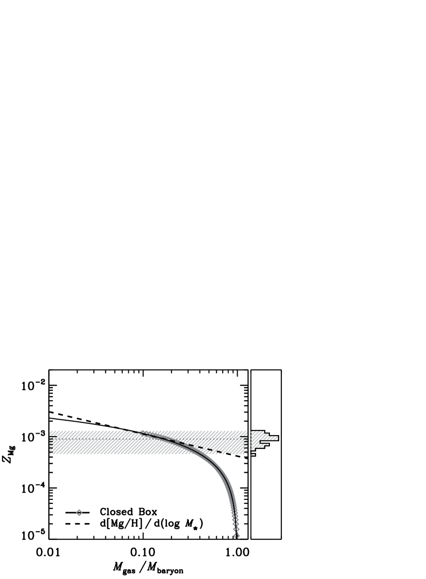
Figure 9.— Comparing the observed relation between [Mg/H] and $M_{\star}$ at fixed $M_{dyn}$ with expectations from a closed box chemical enrichment model. Gray diamonds indicate the closed box model, which assumes instantaneous recycling of the SNe II material, a Salpeter IMF slope above $M=8M_{\odot}$, and the Mg yields of Woosley & Weaver (1995). They show how the Mg-enrichment of the interstellar medium evolves as gas is converted into stars (i.e., as $M_{\rm{gas}}/M_{\rm{baryon}}$ decreases) and can be represented by equation 7 with $y_{\rm{Mg}}=0.0005$ (solid black line). The dashed line shows the observed slope of d[Mg/H]/d(log $M_{\star}$) for galaxies at fixed $M_{dyn}$ (see text for details). The closed box model predicts a similar slope for $Z_{\rm{Mg}}$–$M_{\rm{gas}}/M_{\rm{baryon}}$ as the observed relation for a wide range of residual gas fractions. The gray shaded region and histogram at the right show the range of $Z_{\rm{Mg}}$ spanned by the data. The observed values of [Mg/H] correspond to closed box models with $M_{\rm{gas}}/M_{\rm{baryon}}\sim 0.2$ (i.e., 80% of the gas has been consumed in star formation).

This model tracks the relationship between the fraction of gas consumed in star formation and the Mg-enrichment of the ISM under a set of simple assumptions. We can compare it to the slope of the relation between [Mg/H] and $M_{\star}$ that is observed among the SDSS galaxies at fixed $M_{dyn}$. Table 2 shows that, at fixed $M_{dyn}$ (i.e., fixed $\sigma$ and $R_{e}$), [Mg/H] $\propto 0.35$ $\Delta I_{e}$, while $\log M_{\star}\propto 0.81$ $\Delta I_{e}$. Thus the [Mg/H]–$\log M_{\star}$ relation for a given $M_{dyn}$ should have slope $0.35/0.81=0.43$. This slope is shown in Figure 9 as the dashed line. It closely matches the slope predicted from a closed-box model over a large range of residual gas fractions. This indicates that the observed [Mg/H] variation through the thickness of the FP is at least plausibly consistent with the enrichment expected from the observed change in $M_{\star}$.

The shaded region in Figure 9 shows the range of $Z_{\rm{Mg}}$ spanned by the data, with the dotted line showing the mean value. The distribution of $Z_{\rm{Mg}}$ is indicated by the histogram at the right. In the simple closed box scenario, the observed [Mg/H] values are reached when 10–50% of the baryons are still in the gas phase, i.e., when 50–90% of the gas has been converted into stars.

Recent studies by Mandelbaum et al. (2006) and Zaritsky et al. (2008) find baryon conversion fractions for early-type galaxies of 12–27% and $\sim$10–40%, respectively. However, these studies probe the scale of galaxy groups and clusters. In these large dark matter haloes, the closed box model is obviously incorrect as primeval gas continues to accrete. At early times while the central galaxy is still forming stars, some of this gas may make its way onto the galaxy. This infall is expected to balance star formation (e.g., Dekel et al. 2009). With this type of gas infall, $Z$ rapidly approaches the yield (Binney & Tremaine 1987) and higher absolute abundances are reached sooner, at lower $M_{\rm{gas}}/M_{\rm{baryon}}$. Thus relaxing the assumption of a closed box should lower the conversion fraction necessary to produce the observed levels of [Mg/H]. Furthermore, gas accreted at late times after star formation has ceased will contribute to lower the baryon conversion fraction for the halo as a whole, as it is not used in star formation.

Constructing a more realistic chemical evolution model is beyond the scope of this analysis, but it is interesting to verify that the observed slope of the [Mg/H]–$\log M_{\star}$ relation at fixed $M_{dyn}$ is reasonably consistent with expectations from simple chemical evolution models.

5.3. Alternative Scenarios

We turn now to other possible scenarios for reproducing the observed trends in age, element abundance ratios, and stellar mass surface densities through the FP. Some of these were also considered in Paper III.

5.3.1 IMF Effects

If the IMF is not constant, appropriate variations might be able to produce the observed variations in $\Sigma_{\star}$ and $M_{\star}$ at fixed $\sigma$ and $R_{e}$. There are two simple IMF models: (1) a bottom-heavy IMF that produces more low-mass stars in some galaxies, leading to under-estimates of $\Sigma_{\star}$ and $M_{\star}$ relative to the true mass, and (2) a top-heavy IMF at early times that produces more compact remnants at late times, also leading to under-estimates of $\Sigma_{\star}$ and $M_{\star}$. As discussed in Paper III, neither of these models can explain the full set of observed variations. A bottom-heavy IMF leaves the relative frequencies of SNe II and SNe Ia unchanged and therefore does not produce the observed increase in [Mg/Fe] with decreasing $\Sigma_{\star}$. A top-heavy IMF at early times does increase [Mg/Fe] as required by the observations. However, it also produces an increase in the total production of metals, leading to increases in [Mg/H] and [Fe/H], opposite to the observed trend (see Table 3). Simple models for IMF variation cannot simultaneously reproduce the observed increase in [Mg/Fe] and the decrease in total metal content at low $\Delta I_{e}$.

5.3.2 Differential Dissipation in Galaxy Mergers

In simulations of galaxy mergers, the amount of dissipation changes the profile of the merger remnant by rearranging the distribution stars and dark matter with respect to $R_{e}$ (e.g., Dekel & Cox 2006; Robertson et al. 2006). Variations in the degree of dissipation are therefore another way to produce variations in $\Sigma_{\star}$ and $M_{\star}$ at fixed $\sigma$. However, as discussed in Paper III, the observed trends are not at face value consistent with this picture. Highly dissipational mergers should be more common at early times, when galaxies were in general more gas-rich. This does not naturally square with the observation that less dissipational merger remnants (i.e., galaxies with lower $\Sigma_{\star}$) in fact have older stellar populations at a given $\sigma$ (see Table 3). It is possible to invoke subsequent dissipationless merging as a way to increase $M_{dyn}/M_{\star}$ in systems that form early, but the observed trends extend down to small galaxies with $\sigma\approx 100$ km s^-1, where fewer dissipationless mergers are expected to occur.

5.3.3 Differential Efficiency of Star Formation or Mass-Loss

Other possible models to produce variations in $\Sigma_{\star}$ and $M_{\star}$ at fixed $\sigma$ and $R_{e}$ include mechanisms that modify the efficiency of star formation or of chemical enrichment.

One possibility is that the low-$\Delta I_{e}$ (low-$\Delta\Sigma_{\star}$) galaxies form stars for the same duration of time but overall less efficiently, converting lower fractions of their gas into stars. This successfully produces the lower observed values of [Mg/H] in these objects. It does not, however, produce their higher observed values of [Mg/Fe].

Another possibility is that the low-$\Sigma_{\star}$ galaxies form in lower-mass haloes so that more gas and metals escape in supernova-driven winds during star formation. Like the low-efficiency model above, this model also produces lower $\Sigma_{\star}$ and lower [Mg/H] but does not produce variation in [Mg/Fe].

A third possibility is that the low-$\Sigma_{\star}$ galaxies experience burstier star formation, such that many supernovae go off at once, producing more violent winds. This gives lower overall [Mg/H], as observed, but predicts the wrong trend for [Mg/Fe]; strong winds during bursty star formation should preferentially remove Mg, lowering [Mg/Fe].

It is clear that the combined constraints of lower [Mg/H] and higher [Mg/Fe] in low-$\Sigma_{\star}$ galaxies are powerful tools for discriminating between galaxy formation models. None of the enhanced mass-loss or lower efficiency models discussed in this section naturally produces both trends simultaneously.

5.3.4 Summary of Alternative Models

Faced with meeting both the structural and stellar population constraints provided here and in Paper III, only the premature truncation model seems able to match the data without forcing. The combined strength of these two types of information proves to have surprising constraining power and shows the importance of mapping the stellar population properties into FP space. Putting these two different kinds of information together has created a tight test of galaxy formation models, which at this point seems to leave only one standing: the premature truncation model.

5.4. The Outlying Data Points: Low-$\sigma$, Low-$I_{e}$ Galaxies

In section 3.2, we identified three galaxy bins that deviate significantly from what one would expect from a smooth extrapolation of the other data. These are the lowest-$\Delta I_{e}$ bins ($-0.25<\Delta I_{e}<-0.15$) for each of the three lowest-$\sigma$ bins ($1.86<\log\sigma<2.00$, $2.00<\log\sigma<2.09$, and $2.09<\log\sigma<2.18$), which are outlined by black circles in Figures 3, 4, 6, and 7. We consider here several possible explanations for these galaxies.

These galaxies stand out most clearly in Figure 4, where their [Mg/Fe] values appear much lower than expected, particularly for the lowest $\sigma$ bin. Their age and [Fe/H] values appear relatively consistent with the other data in Figure 2, but become more discrepant when curvature is allowed in the age fit of equation 2, as can be seen in Figure 6. To summarize, these outliers have ages that are too old, [Mg/H] abundances that are too low, and [Mg/Fe] values that are way too low compared to what one would expect from an extrapolation of the other data. The low values of both [Mg/H] and [Mg/Fe] suggest that these galaxies lost a larger fraction of their SNe II-enriched material than did their counterparts at the same $\sigma$ with higher $\Delta I_{e}$.

One possibility is that these galaxies are substantially affected by sample selection effects. They populate the part of galaxy parameter space that suffers from serious incompleteness (Figure 1). However, is is not clear how this would produce the observed deviations in stellar population properties. The galaxy bins contain enough galaxies to produce adequate S/N in the stacked spectra (Table 1). They are mostly populated by galaxies from the lower-redshift ($0.04<z<0.05$) portion of our sample. However, the quiescent, passive galaxy population we consider here should not have changed significantly in the $\sim 500$ Myr between $z=0.08$ and $z=0.04$ (particularly those at low $\Delta I_{e}$, which have SSP ages $>7$ Gyr), making it difficult to explain the observed deviations through the effects of evolution within the sample. The higher-redshift galaxies in these bins may be erroneously assigned to the bins due to measurement errors in $\sigma$ or in $\Delta I_{e}$. These galaxies should contribute spectra that are representative of the galaxy properties in other, higher-$\sigma$, higher-$\Delta I_{e}$ bins. If the outliers are caused by erroneous bin assignment, they should represent linear combinations of galaxy properties of other bins. This is not the case; these bins have the lowest observed values of [Mg/H] and combined [Mg/Fe] and age values that differ substantially from all other galaxy bins (see Figures 3 and 4).

A second possibility is that, if the stellar population properties of satellite galaxies differ substantially from those of similar galaxies that are central to their haloes, the observed deviations in these bins could be due to a higher contribution from satellite galaxies. We use the group catalogs of Yang et al. (2007) to identify galaxies which have the highest $M_{\star}$ in their group and identify these as central galaxies, while other galaxies are classified as satellites. The satellite fraction, which is less than one-third in most of the galaxy bins, increases to a maximum of two-thirds in the lowest-$\sigma$, lowest-$\Delta I_{e}$ bin. However, a preliminary analysis of the stellar population properties of central galaxies as compared to satellite galaxies with the same $\sigma$ and $\Delta I_{e}$ suggests that the two types of galaxies have similar stellar populations (see also Cooper et al. 2009). Furthermore, the satellite fraction of a bin depends more strongly on $\sigma$ than on $\Delta I_{e}$; the highest satellite fractions are found in the three bins with $1.86<\log\sigma<2.00$ and $\Delta I_{e}<+0.05$, rather than the three bins with $1.86<\log\sigma<2.18$ and $\Delta I_{e}<-0.15$. We reserve a more detailed analysis of the stellar populations of satellite versus central galaxies for a future paper, but note here that our preliminary work on this topic suggests that it cannot account for the observed outliers.

A third possibility is that the outliers are due to differences in their susceptibility to feedback. These galaxies, with the lowest values of $\Delta I_{e}$ and low values of $\sigma$, are exactly those galaxies which we would expect to be most strongly affected by feedback. They have the shallowest potential wells (low $\sigma$) and the least-concentrated mass profiles (low $\Delta I_{e}$ and low $\Delta\Sigma_{\star}$). The outlying galaxies behave in exactly the way predicted for galaxies that experience substantial mass-loss driven by SNe II feedback (see section 5.3.3), showing both lower than expected values of [Mg/H] and [Mg/Fe]. The most deviant galaxies are those in the lowest $\sigma$ bin, which would be the most vulnerable to the removal of Mg-enriched material. Moreover, the anomalies increase at lower $\sigma$, futher targeting low $\sigma$ and feedback as the cause.

A problem with this line of argument is that it is not clear why this effect would kick in suddenly at low $\Delta I_{e}$ (there is no indication of deviation for galaxies with similar $\sigma$ and $\Delta I_{e}>-0.15$). This could be explained if, in addition to having the shallowest gravitational potentials, these galaxies have the burstiest star formation histories. The observed low values of [Mg/Fe] in these galaxies require the preferential loss of Mg-enriched material over Fe-enriched material. Multiple short bursts of star formation would maximize Mg ejection through large numbers of simultaneous SNe II, while the more extended production of Fe by SNe Ia would be less efficient at expelling enriched gas, leaving the Fe in the ISM to be incorporated in the next burst of star formation. Combining bursty star formation histories with shallow potential wells could produce the dramatic transition observed between the main population of early-type galaxies and these outliers.

6. Discussion

6.1. Physical Mechanisms for Truncating Star Formation

The premature truncation model appears to reproduce the complex ensemble of galaxy data presented in this series of papers. Multiple physical mechanisms have been proposed that could provide such a truncation scenario, which we discuss briefly here.

6.1.1 Quenching in Infalling Satellites

One possible truncation mechanism for satellite galaxies is the rapid quenching of star formation when a satellite falls into a massive halo and is stripped of gas (e.g., Gunn & Gott 1972; Lea & De Young 1976; Gisler 1976). This explanation predicts that the prematurely truncated galaxies (those with lower $\Delta I_{e}$) at a given $\sigma$ should be satellites in massive haloes, and that the lowest-$\Delta I_{e}$ galaxies are those that were accreted into massive haloes at the earliest times. There is some evidence that, at fixed $\sigma$, galaxies in denser environments have slightly older ages than those in the field (e.g., Trager et al. 2000b; Thomas et al. 2005; Clemens et al. 2006; Bernardi et al. 2006; Smith et al. 2008b; Cooper et al. 2009). However, it is not clear that these galaxies can be associated with the low-$\Delta I_{e}$ galaxies—they do not necessarily also show lower metallicities and higher [Mg/Fe]. There is observational evidence that this type of quenching may proceed slowly in massive galaxies (Wolf et al. 2009) and may not be adequately abrupt to produce the high [Mg/Fe] seen in high-$\sigma$ galaxies with low $\Delta I_{e}$. Furthermore, the majority of our sample galaxies are central to their haloes; two thirds of our sample galaxies are identified as the brightest group galaxies in the Yang et al. (2007) catalog of SDSS galaxy groups.

The role of satellite quenching as a mechanism for premature truncation can and should be addressed in future work that distinguishes between satellite galaxies and those that are central to their dark matter haloes, as well as studying these trends in $\Delta I_{e}$ as a function of environment.

6.1.2 AGN-driven Quenching

Another possible truncation mechanism is very powerful feedback, in which a substantial quantity of the ISM is heated and removed from the galaxy potential well before it can form stars. AGN may be able to heat and remove substantial fractions of the ISM (Granato et al. 2004; Scannapieco & Oh 2004; Di Matteo et al. 2005; Springel et al. 2005; Hopkins et al. 2008), possibly with an additional boost to the momentum-driven winds from AGN-triggered star formation (Silk & Nusser 2010). As an example, Nesvadba et al. (2007) present optical and radio observations of two massive $z=3.5$ galaxies with strong radio jets and calculate that the mass-loading of the jet material may represent several times $10^{10}M_{\odot}$ of ISM. Such objects may be evidence of powerful AGN feedback in action. Interestingly, Hopkins et al. (2007a) find that simulations of black hole growth through major-merger-driven accrection predict a two-dimensional “Black Hole Fundamental Plane” (BHFP), which agrees well with observations (Hopkins et al. 2007b). However, black hole growth in the simulations is regulated by the conditions needed for feedback to power a pressure-driven outflow, such that the resulting black hole mass depends on the details of the local potential and is surprisingly insensitive to other merger properties. In this paradigm, $M_{BH}$ should be unique for a given combination of $\sigma$ and $R_{e}$. It is therefore not obvious how AGN-driven feedback would vary in such a way as to produce the observed premature truncation in galaxies at fixed $\sigma$ and $R_{e}$.

6.1.3 Supernova-driven Quenching and Differential Halo Assembly

Supernova feedback provides another mechanism for injecting energy into the ISM. In a model where the SN-driven outflow rate is comparable to the star formation rate, SN feedback may be relevant for driving galactic winds and outflows at all mass scales (Silk 2003; Pipino & Matteucci 2004), although many galaxy evolution models require some further feedback from other sources such as AGN in order to fully quench star formation in massive galaxies (e.g., Hatton et al. 2003; Croton et al. 2006; Bower et al. 2006). If some galaxies experience stronger SN feedback for a given star formation rate, for example due to differences in mass-loading in the winds (e.g., Pipino et al. 2009b), or if galaxies of a given mass form stars at different rates (e.g., due to different accretion histories), the galaxies with stronger feedback or more rapid star formation may shut down star formation earlier, resulting in low $\Delta I_{e}$ galaxies with older ages, higher [Mg/Fe], and lower total metal enrichment.

Another possibility is that the low $\Delta I_{e}$ galaxies did not form the majority of their stars in situ, but instead assembled hierarchically at early times from many smaller galaxies. These small galaxies might be more susceptible to supernova feedback because they have shallower potential wells (White & Rees 1978; Dekel & Silk 1986; White & Frenk 1991; Benson et al. 2003). This process could shut down star formation at earlier times and lead to the observed older ages and higher [Mg/Fe] of their massive descendents, as compared to galaxies at the same $\sigma$ with higher $\Delta I_{e}$, which may have formed more of their stars in situ in massive haloes. A galaxy which formed in many smaller pieces would also have lower metallicity, both because its ISM experienced fewer generations of stellar processing resulting in a lower effective yield, and because SN feedback would be more effective at removing metal-enriched gas from the galaxy.

Differences in halo assembly histories are well-modeled by cosmological simulations. Thus the new generation of semi-analytic models, which include predictions for $\sigma$ and $R_{e}$ based on merger simulations, may prove important tools for testing assembly-dependent truncation mechanism. The successful modeling of these trends probably requires an improved treatment of satellite galaxies in the new generation of semi-analytic models (e.g., Guo et al. 2010) over previous models, which often fail to correctly model the stellar populations of satellite galaxies (Font et al. 2008; Kimm et al. 2009; Pipino et al. 2009a).

6.1.4 Quenching in Massive Dark Matter Haloes

Yet another mechanism is quenching by massive haloes (e.g., Birnboim & Dekel 2003; Kereš et al. 2005; Cattaneo et al. 2008), when haloes pass over a critical mass threshold ($M_{crit}$) and shock-heated gas accreting onto them can no longer cool efficiently. This process appears to be able to quench star formation in haloes with $M_{halo}\sim 10^{12}$–$10^{13}M_{\odot}$ (Birnboim et al. 2007). When supplemented with gravitational heating from continued cosmological gas accretion, this effect may be able to truncate star formation in more massive haloes as well (Dekel & Birnboim 2008). In this scenario, the observed variations through the FP could be due to stochastic variations in the halo mass assembly history. If galaxies with the same $\sigma$ and $R_{e}$ today exist in haloes that passed over $M_{crit}$ at different times, or if mass was accreted differently onto these haloes, affecting the cooling rate, these galaxies could have different star formation histories. The low-$\Delta I_{e}$ galaxies, which were truncated earlier, would be those that crossed this critical halo mass threshold at earlier times. This scenario should also be quantitatively testable with semi-analytic models.

6.1.5 Summary of Truncation Mechanisms

These various scenarios for premature truncation make predictions about how a galaxy’s status as a central versus a satellite, the local environment, central black hole mass, dark matter halo mass, and mass assembly history should vary at fixed $\sigma$ for galaxies with different star formation histories and in different parts of FP space. A combination of further observational programs and improved semi-analytic models for galaxy formation (that can track values of $\sigma$ and $R_{e}$ for galaxies in a cosmological context) should be able to distinguish between these different truncation mechanisms. The analysis presented here makes it possible to identify galaxies that have experienced premature truncation, providing a powerful tool for exploring the quenching of star formation in galaxies.

6.2. The Effects of Dry Merging

The build-up of $L\sim L^{*}$ red galaxies since $z\sim 1.5$ (Bell et al. 2004; Faber et al. 2007) appears to require a contribution from dissipationless “dry” mergers between galaxies that have already quenched star formation and occupy the red sequence (e.g., Faber et al. 2007). In this section, we explore the effects of dry merging on the location of galaxies in FP space and the observed stellar population trends. We consider the two extremes of dry merging: equal-mass major mergers between identical progenitor galaxies and the build-up of mass through a series of minor mergers accreting onto a massive central galaxy. These cases bracket the range of merger mass ratios.

The scenario of mass-doubling through equal-mass dry mergers has been explored by Boylan-Kolchin et al. (2005, 2006) using N-body simulations. The models use empirically-motivated initial conditions for the galaxies, combined with Navarro et al. (1997) dark matter haloes which are allowed to evolve actively through the course of the simulation. More recently, Naab et al. (2009) have modeled the effects of mass-doubling through a large number of minor mergers in a cosmologically-motivated hydrodynamical simulation of a galaxy which has no mergers with mass ratios greater than 1:8 after $z=3$. Naab et al. (2009) also present a simple analytic argument for the way in which $\sigma$, $R_{e}$ and stellar density should scale in mergers, based on the virial theorem. We use these studies here to consider the effects of dry merging on the observed stellar population trends throughout FP space.

Boylan-Kolchin et al. (2006) find that equal mass dry mergers between galaxies that lie on the FP result in merger remnants that also lie on the FP. The merger remnants have velocity dispersions ($\sigma_{f}$) similar to those of the progenitor galaxies ($\sigma_{i}$), with $\sigma_{f}\approx 1.2\sigma_{i}$ for the most probable orbital parameters and $\sigma_{f}\approx 1.0\sigma_{i}$ for radial orbits. The remnant effective radii change more, with $R_{f}\approx 1.6R_{i}$ for the most probably orbital paramters and $R_{f}\approx 2.5R_{i}$ for radial orbits. This is in reasonable agreement with the simple analytic model of Naab et al. (2009), who argue that equal-mass dry mergers should produce $\sigma_{f}=\sigma_{i}$ and $R_{f}=2R_{i}$.

If we assume that the progenitors are identical, lie on the FP, and have the stellar populations predicted for their location in FP space, then the resulting merger remnant will have the same stellar populations as the progenitors, roughly the same $\sigma$, a larger $R_{e}$, and will lie on the FP midplane (i.e., it will have $\Delta I_{e}=0$). This is entirely consistent with the observations in Paper II, which show that galaxies with the same $\sigma$ but different $R_{e}$ on the FP midplane have the same stellar populations. The virial scalings of Naab et al. (2009) also predict almost no motion off the FP midplane, with $(\Delta I_{e})_{f}=+0.06$ in the merger remnant, assuming the progenitors had $(\Delta I_{e})_{i}=0.0$. Thus equal-mass dry merging will preserve the stellar population trends identified in this series of papers and will not tend to move galaxies off the FP midplane.

Applying the virial scaling arguments of Naab et al. (2009) to mass doubling through minor mergers implies $\sigma_{f}=0.5\sigma_{i}$ and $R_{f}=4R_{i}$. Assuming the progenitors lie on the FP with $(\Delta I_{e})_{i}=0.0$, the resulting remnant after many minor mergers should have $(\Delta I_{e})_{f}=-0.12$. Thus minor mergers will slowly move galaxies off the FP toward lower surface brightnesses, while also lowering $\sigma$ and dramatically increasing $R_{e}$.

If the progenitors have the stellar populations inferred from their location in FP space, the accretion of stars from the lower-$\sigma$ galaxies will tend to lower the SSP age of the galaxy, while also lowering [Mg/Fe], [Fe/H], and [Mg/H]. However, the hydrodynamical simulations of Naab et al. (2009) showed that the majority of stars accreted from small satellites wind up at large radius. At $z=0$, accreted stars account for $\sim 1/7$ of the stars inside 1 kpc, beyond which the relative contribution of accreted stars slowly increases. This means that stellar populations sampled by the SDSS spectral fibers are dominated by the in situ component of stars, not the accreted stars. Thus the stellar population of the merger remnant as observed through the SDSS fiber will not change dramatically from that of the massive progenitor galaxy.

This means that the net effect of a series of minor mergers will be to move the galaxy to lower $\sigma$ and higher $R_{e}$, while hardly changing the central stellar population. From the virial scaling argument above, these galaxies will lie slightly off the FP at lower $\Delta I_{e}$. Because the main progenitors started out with higher $\sigma$, they should have older ages and higher [Mg/Fe] than other galaxies with the same $\sigma_{f}$ on the FP midplane. This is in the same direction as the observed trends at fixed $\sigma$ to lower $\Delta I_{e}$. However, they should also have higher [Fe/H] and higher [Mg/H], which is in the opposite direction from the observed trends. If we relax the aperture assumption and allow the accreted low-mass galaxies to contribute substantially to the light sampled by the SDSS fiber, they will tend to contribute stars that are younger with lower [Mg/Fe], lower [Fe/H], and lower [Mg/H]. This improves the match to the observed [Fe/H] and [Mg/H] values, but washes out the trends with age and [Mg/Fe].

All in all, it appears that modest quantities of dry merging will leave the observed stellar population trends through FP space essentially unchanged. Very large numbers of minor mergers may tend to smear out some of the observed trends.

7. Conclusions

Papers I and II presented a detailed analysis of the stellar population properties of quiescent early-type galaxies. These population properties were mapped through two familiar early-type galaxy scaling relations: the color-magnitude relation (Paper I) and the Fundamental Plane (Paper II). Paper III supplemented that work with a detailed study of galaxy mass-to-light ratios, showing that stellar population mass-to-light ratio effects do not contribute the majority of the observed variation in $\Delta I_{e}$. These works illustrated that the stellar population properties (and by inference the star formation histories) of these galaxies form a two-parameter family. Furthermore, this two-parameter family maps onto the large-scale structural properties of the galaxies.

In this work, we have presented what we feel is the clearest and most intuitive representation of the relevant structural properties for early-type galaxies: $\sigma$ and $\Delta I_{e}$. We have shown how the various stellar population parameters map onto this structural space, which corresponds to a cross-section projected through the FP. We have also explored in detail the co-variation of mean light-weighted age, [Fe/H], [Mg/H], and [Mg/Fe] among early-type galaxies. By combining these stellar population results with the mass information from Paper III, we have presented a plausible scenario for early-type galaxy star formation histories that is consistent with the multidimensional properties of the data. Our main conclusions can be summarized as follows:

• The stellar populations of quiescent early-type galaxies form a 2D family, similar to the age-metallicity hyperplane of Trager et al. (2000a). In the first dimension of the parameter space, mean light-weighted age, [Fe/H], [Mg/H], and [Mg/Fe] all increase together. In the second dimension of the parameter space, age and [Mg/Fe] increase while [Fe/H] and [Mg/H] decrease.

• This 2D family of stellar population properties can be mapped onto a cross-section projected through the FP, parameterized in this work by $\sigma$ and $\Delta I_{e}$. The first dimension of the parameter space maps onto $\sigma$, such that age, [Fe/H], [Mg/H], and [Mg/Fe] all increase with increasing $\sigma$. The second dimension maps onto $\Delta I_{e}$ at fixed $\sigma$, such that as $\Delta I_{e}$ increases, [Fe/H] and [Mg/H] increase while age and [Mg/Fe] decrease.

• Given the systematic behavior described in conclusion 2, it is possible to estimate the stellar population properties of a quiescent early-type galaxy based on its location in FP space. Equations 2–5 quantify this mapping. They are shown to reproduce the binned observed stellar population properties to roughly within the observational errors.

• Paper III showed that variations in $\Delta I_{e}$ are primarily due to variations in stellar mass surface density, $\Delta\Sigma_{\star,IMF}$. This means that the observed stellar population variations through the thickness of the FP correlate with variations in $\Delta\Sigma_{\star,IMF}$, or alternatively with variations in $\Delta M_{dyn}/M_{\star,IMF}$. At fixed $\sigma$, galaxies with younger ages, lower [Mg/Fe], and greater total metal enrichment (i.e., higher [Fe/H] and [Mg/H]) also have larger $\Sigma_{\star,IMF}$ and formed more stars.

• The observed stellar population variations can be interpreted in terms of star formation histories where the start time and duration of star formation both depend on $\sigma$ (e.g., a “staged star formation” model), but in which there are also systematic variations in the duration of star formation ($\Delta t_{SF}$) at fixed $\sigma$.

• At fixed $\sigma$, galaxies with longer duration star formation have higher $\Sigma_{\star,IMF}$ and higher total $M_{\star,IMF}$ at fixed $R_{e}$. They also are more enhanced in both Fe and Mg, with lower [Mg/Fe] than their counterparts that experienced shorter duration star formation. This strongly suggests that they have experienced higher “conversion efficiencies” of turning their gas into stars.

• The observed pattern, in which longer duration star formation corresponds to the production of more stars, while shorter duration star formation produces fewer stars, leads us to propose a premature truncation model for quiescent galaxy star formation histories. In this model, star formation proceeds similarly for all galaxies of the same $\sigma$ but is truncated at different times. Thus some galaxies are shut down while their formation process is less complete, leaving them with fewer total stars, lower $\Sigma_{\star,IMF}$, and lower metal abundances.

References

- Adelman-McCarthy et al. (2008) Adelman-McCarthy, J. K., et al. 2008, ApJS, 175, 297
- Adelman-McCarthy et al. (2006) —. 2006, ApJS, 162, 38
- Anders & Grevesse (1989) Anders, E., & Grevesse, N. 1989, Geochim. Cosmochim. Acta, 53, 197
- Arimoto & Yoshii (1987) Arimoto, N., & Yoshii, Y. 1987, A&A, 173, 23
- Bell et al. (2004) Bell, E. F., et al. 2004, ApJ, 608, 752
- Benson et al. (2003) Benson, A. J., Bower, R. G., Frenk, C. S., Lacey, C. G., Baugh, C. M., & Cole, S. 2003, ApJ, 599, 38
- Bernardi et al. (2006) Bernardi, M., Nichol, R. C., Sheth, R. K., Miller, C. J., & Brinkmann, J. 2006, AJ, 131, 1288
- Binney & Tremaine (1987) Binney, J., & Tremaine, S. 1987, Galactic dynamics (Princeton University Press, Princeton, NJ)
- Birnboim & Dekel (2003) Birnboim, Y., & Dekel, A. 2003, MNRAS, 345, 349
- Birnboim et al. (2007) Birnboim, Y., Dekel, A., & Neistein, E. 2007, MNRAS, 380, 339
- Blanton et al. (2005) Blanton, M. R., et al. 2005, AJ, 129, 2562
- Bower et al. (2006) Bower, R. G., Benson, A. J., Malbon, R., Helly, J. C., Frenk, C. S., Baugh, C. M., Cole, S., & Lacey, C. G. 2006, MNRAS, 370, 645