Water/Icy Super-Earths: Giant Impacts and Maximum Water Content

Abstract

Water-rich super-Earth exoplanets are expected to be common. We explore the effect of late giant impacts on the final bulk abundance of water in such planets. We present the results from smoothed particle hydrodynamics simulations of impacts between differentiated water(ice)-rock planets with masses between 0.5 and 5 M_⊕ and projectile to target mass ratios from 1:1 to 1:4. We find that giant impacts between bodies of similar composition never decrease the bulk density of the target planet. If the commonly assumed maximum water fraction of 75wt% for bodies forming beyond the snow line is correct, giant impacts between similar composition bodies cannot serve as a mechanism for increasing the water fraction. Target planets either accrete materials in the same proportion, leaving the water fraction unchanged, or lose material from the water mantle, decreasing the water fraction. The criteria for catastrophic disruption of water-rock planets are similar to those found in previous work on super-Earths of terrestrial composition. Changes in bulk composition for giant impacts onto differentiated bodies of any composition (water-rock or rock-iron) are described by the same equations. These general laws can be incorporated into future N-body calculations of planet formation to track changes in composition from giant impacts.

1. Introduction

Super-Earths, massive terrestrial exoplanets in the regime $\lesssim$ 10 M_⊕, are expected to come in a diversity of bulk compositions. Both planet formation theory and comparative planetology stand to benefit from distinguishing super-Earths of different composition. It is especially valuable to know how water-rich such planets could be. Water is abundant in protoplanetary disks, but it is also very volatile, so the details of the planet formation (and post-formation) process can be crucial in determining the distribution of water-rich planets by bulk composition and orbit.

The catalog of observed extrasolar planets now includes more than 400 members. Of these, more than 70 planets have been observed transiting their parent star. Until recently, the only known transiting planets were similar in mass to either Jupiter or Neptune. With CoRoT-7b (Léger et al., 2009; Queloz et al., 2009) and GJ1214b (Charbonneau et al., 2009), we now have the first observed transits of planets in the super-Earth mass regime. Many more detections are expected in the near future from the Kepler mission (Borucki et al., 2009). A transit observation provides a determination of the planet’s radius as well as the inclination angle of the planet’s orbit with respect to the line of sight. When combined with the mass determined from radial velocity measurements, the mean density of the planet is derived.

Given the bulk density of a super-Earth, it is possible to estimate a range of possible internal compositions, from rocky/iron terrestrial planets with small radii for a given mass, to icy and gas rich planets with much larger radii (e.g., Valencia et al., 2006, 2007; Fortney et al., 2007; Seager et al., 2007). The precise composition of the planet cannot be determined from internal structure models alone because of the degeneracy in the mass–radius relationship for various compositions. However, with precise measurements of radius and mass (uncertainties $\lesssim$ 5% and 10%, respectively), one can distinguish an icy/rocky super-Earth from a rocky/iron super-Earth (Valencia et al., 2007).

The mass and radius measurements for CoRoT-7b, 4.8 $\pm$ 0.8M_⊕ and 1.68 $\pm$ 0.09$R_{\oplus}$, respectively, are consistent with a planet of terrestrial composition (Léger et al., 2009; Queloz et al., 2009). GJ1214b, with a similar mass of 6.55 $\pm$ 0.98$M_{\oplus}$, has a radius of 2.678 $\pm$ 0.13$R_{\oplus}$, implying the presence of a thin hydrogen/helium envelope around a core composed primarily of ice or, alternatively, a thick hydrogen/helium envelope around a rocky core (Charbonneau et al., 2009).

Further constraints on the compositions of transiting super-Earths can be obtained from a theoretical understanding of planet formation. Ida & Lin (2004) and Mordasini et al. (2009) have applied detailed models of planet formation to the generation of synthetic populations. Figueira et al. (2009) have combined the planet formation model of Mordasini et al. (2009) with simplified interior structure models to determine a statistical distribution of possible compositions for the transiting hot Neptune GJ436b, excluding the possibilities that the planet is either an envelope-free water planet or a rocky planet with a hydrogen/helium envelope. Such constraints represent a major triumph for planet formation models. However, all current models neglect the potentially important effects of multiple embryo formation and giant impacts.

Giant impacts are thought to have played a major role in shaping the planets in our solar system. Such events have been shown to explain the high bulk density of Mercury in the inner solar system (Benz et al., 1988, 2007), the formation of the Haumea collisional family in the outer solar system (Brown et al., 2007; Leinhardt et al., 2010), and properties of several planets in between. In fact, giant impacts are an inevitable consequence of the core accretion model of planet formation (e.g., Wetherill, 1994). Marcus et al. (2009) developed scaling relations to determine the outcome of giant impacts between planets of terrestrial composition. They extended the catastrophic disruption criteria of Stewart & Leinhardt (2009) into the super-Earth mass regime and provided a power-law relationship for the iron mass fraction of the largest impact remnant given target mass, impactor mass, and impact velocity. These laws were then combined with simple dynamical arguments to constrain the minimum radius of super-Earths as a function of mass (Marcus et al., 2010).

Ultimately, we want to know what the distribution of super-Earths of different bulk composition looks like in the mass-radius diagram. The work by Marcus et al. (2010) defines the theoretically anticipated lower envelope of that distribution. This Letter attempts to similarly define an upper envelope, if one does occur, that might separate water planets with no hydrogen/helium envelopes from mini-Neptunes with hydrogen/helium envelopes around an icy/rocky or just rocky core. We follow the same premise, that well-defined initial bulk compositions can be modified by late-time giant impacts to reach either of the envelopes of the mass-radius distribution of super-Earths.

2. Method

We performed a series of more than 100 simulations using the smoothed particle hydrodynamics (SPH) code GADGET (Springel, 2005), modified to read tabulated equations of state (EOS, Marcus et al., 2009). For more details on using this scheme for giant planetary impact simulations see Marcus et al. (2009, 2010).

We considered targets ranging in mass from 0.5 $M_{\oplus}$ to 5 $M_{\oplus}$. The mass of the planets was 50% H₂O and 50% serpentine (Mg₃Si₂O₅(OH)₄, $\sim$ 11-15% H₂O by mass) with a bulk density of $2.2-3.6$ g cm^-3. The higher bulk densities for the largest mass planets reflect the formation of dense high-pressure polymorphs of ice and the corresponding smaller total planetary radii. This composition is consistent with the protosolar ice/rock ratio of $\sim$ 2.5 (Guillot, 1999) and more ice-rich than the composition of the dwarf planets and large KBOs in the outer solar system (McKinnon et al., 2008). The serpentine EOS was tabulated from the code ANEOS (Thompson & Lauson, 1972), with input parameters taken from Brookshaw (1998). The ice EOS was the tabulated 5-Phase equation of state for H₂O (Senft & Stewart, 2008). Bodies were initialized with fixed temperature profiles from Fu et al. (2010) and all materials are hydrodynamic. Each body had 25000-100000 SPH particles. A subset of the simulations was run at twice this resolution, with identical results.

The projectile-to-target mass ratios were 1:4, 1:2, and 1:1. Because the outcome of giant impacts has been shown to depend very strongly on impact angle (Agnor & Asphaug, 2004; Marcus et al., 2009), we considered impact parameters of $b$=0 (0^∘, head-on), $b$=0.5 (30^∘), and $b$=0.707 (45^∘).

3. Results

3.1. Catastrophic Disruption Criteria and Icy Mantle Stripping

Giant collisions that are near or directly head-on (zero impact parameter $b$) of sufficient energy lead to disruption and net erosion. The criterion for catastrophic disruption is an impact condition that leads to a largest remnant with half the original combined colliding mass. In the disruption regime, the mass of the largest impact remnant is a function of the reduced mass kinetic energy divided by the total colliding mass, scaled by the catastrophic disruption criteria $Q^{*}_{\rm{RD}}$, a scaling factor that depends primarily on the total colliding mass and the impact velocity. The reduced mass kinetic energy, scaled to the total colliding mass is $Q_{\rm{R}}=\frac{1}{2}\mu V_{\rm{i}}^{2}/M_{\rm{tot}}$, where $\mu$ is the reduced mass, $V_{\rm{i}}$ is the impact velocity, and M_tot is the total mass. The size- and velocity-dependent catastrophic disruption criteria for weak bodies in the gravity-dominated regime are given by (Stewart & Leinhardt, 2009, Equation 2)

$$Q^{*}_{\rm{RD}}=10^{-4}R_{\rm{C1}}^{1.2}V_{\rm{i}}^{0.8}.$$ (1)

Here $R_{\rm{C1}}$ is the radius of a spherical body with mass $M_{\rm{tot}}$ and a mean density of 1 g cm^-3. These disruption criteria, originally fit to $N$-body impact simulations between planetesimals, were shown by Marcus et al. (2009) to extend into the super-Earth mass regime for bodies of terrestrial composition. In Figure 1, the fitted $Q^{*}_{\rm{RD}}$ values for collisions between icy planets are shown as a function of $R_{\rm{C1}}$. The disruption criteria of Stewart & Leinhardt (2009) fit the data for ice-rock planets as well, predicting $Q^{*}_{\rm{RD}}$ to within a factor of 2 of the hydrocode calculations for head-on ($b$=0) impacts. The predicted $Q^{*}_{\rm{RD}}$ is smaller than the hydrocode calculations for head-on impacts; however, the hydrocode calculations do not include material strength which biases the value of $Q^{*}_{\rm{RD}}$ downward (e.g., see Leinhardt & Stewart, 2009). Oblique impacts are discussed below. Thus, these disruption criteria are largely independent of the internal compositions of the colliding bodies.

Stewart & Leinhardt (2009) found a linear relationship between $Q_{\rm{R}}$ and the mass of the largest remnant scaled to the total colliding mass:

$$M_{\rm{lr}}/M_{\rm{tot}}=-0.5(Q_{\rm{R}}/Q^{*}_{\rm{RD}}-1)+0.5\,.$$ (2)

In Figure 2, the mass of the largest remnant, scaled to the total colliding mass, is shown as a function of the reduced mass kinetic energy. The linear relationship still holds for super-Earth planets consisting largely of ice (dotted line). Thus, this scaling relationship should be valid for all solid planetary bodies, regardless of the details of the internal structure.

In these disruptive simulations, some of the icy mantle is removed, leading to an increase in bulk density. The rocky core mass fraction of the largest impact remnant is given by a power law of $Q_{\rm{R}}$/$Q^{*}_{\rm{RD}}$,

$$M_{\rm{core}}/M_{\rm{lr}}=0.5+0.25(Q_{\rm{R}}/Q^{*}_{\rm{RD}})^{1.2},$$ (3)

shown by the dashed line in Figure 2.

3.2. Effect of the impact parameter: Disruption versus Hit and Run

High velocity head-on impacts fall in the disruption regime discussed above. As the impact parameter increases and the impacts become more grazing, a different regime emerges. The hit-and-run impact events described by Agnor & Asphaug (2004) and Marcus et al. (2009) also occur for the planets presently considered. This regime is defined by a sharp discontinuity between merging impacts at low velocity and high velocity collisions in which the impactor grazes the target and both bodies escape the encounter largely intact.

Figure 3 shows the accretion efficiency, $\xi$, as a function of the impact velocity scaled to the mutual escape velocity ($v_{\rm{esc}}^{2}=2G(M_{\rm{targ}}+M_{\rm{proj}})/(R_{\rm{targ}}+R_{\rm{proj}})$). The accretion efficiency is defined as the difference between the mass of the largest impact remnant and the target mass, divided by the mass of the impactor (Asphaug, 2009):

$$\xi\equiv\frac{M_{\rm{lr}}-M_{\rm{targ}}}{M_{\rm{proj}}}.$$ (4)

The impact velocity of the transition between accretion and hit-and-run depends on the impact angle and the projectile-to-target mass ratio, but always falls in the range $v_{\rm{i}}\sim 1.1-1.5v_{\rm{esc}}$. For the icy planets, all of the $b$=0.7 simulations transitioned from merging to hit-and-run and remain in the hit and run regime for the range of impact velocities considered here. The simulations with $b$=0 smoothly transitioned from merging to disruption. For $b$=0.5, there is a small hit-and-run regime between merging and disruption.

In the hit-and-run regime, catastrophic disruption may still occur at extremely high impact velocities. Figure 1 includes the calculated catastrophic disruption criteria versus combined spherical radius for 30^∘ impacts with mass ratios of 1:2 and 1:4; the predicted $Q^{*}_{\rm{RD}}$ using Equation (1) are only 20% larger on average when accounting for the different critical impact velocities. The 30^∘ impacts with mass ratio of 1:1 and all the 45^∘ impacts resulted in hit and run up to $4V_{\rm{esc}}$, and we could not derive a $Q^{*}_{\rm{RD}}$.

30^∘ impact conditions typically result in $Q^{*}_{\rm{RD}}$ values larger than that for head-on impacts by a factor of $\sim$2. However, there is also a non-trivial dependence on the mass-ratio of the colliding bodies. The combined factors of mass ratio and impact angle are complicated enough to warrant a future dedicated study for the boundary between the disruption and hit-and-run regimes.

3.3. Two Models for Mantle Stripping in a Differentiated Body

Combining the results of the simulations of collisions between rock/ice super-Earths discussed above with the collision simulations of iron/rock super-Earths from Marcus et al. (2009), we construct two general models for collisional mantle stripping in a two material, differentiated planet. In the first one, we begin by calculating $Q^{*}_{\rm{RD}}$ from Equation (1), followed by the expected mass of the largest remnant from Equation (2). In this model, we assume that all escaping mass is the lightest material; that is, the cores of the two bodies merge. If the combined mass of the two cores is less than the mass of the largest remnant, mantle material is added until the total mass reaches $M_{\rm{lr}}$. Given the core masses of the target and projectile, $M_{\rm{core,targ}}$ and $M_{\rm{core,proj}}$, the mass of the final post-impact core is then

$$M_{\rm{core}}=\rm{min}(M_{\rm{lr}},M_{\rm{core,targ}}+M_{\rm{core,proj}}).$$ (5)

In the second model, the first step is again to calculate $Q^{*}_{\rm{RD}}$ and the expected mass of the largest remnant from Equations (1) and (2), respectively. In the accretion regime, where the mass of the largest remnant is larger than the target mass, we assume that core material is accreted first from the impactor followed by mantle material. The mass of the final post-impact core is then

$$M_{\rm{core}}=M_{\rm{core,targ}}+\rm{min}(M_{\rm{core,proj}},M_{\rm{lr}}-M_{\rm{targ}}).$$ (6)

In the disruption regime, where the mass of the largest remnant is smaller than the target mass, we assume that the material is stripped away from the target in spherical shells, beginning with mantle material only. The core mass of the largest remnant is

$$M_{\rm{core}}=\rm{min}(M_{\rm{core,targ}},M_{\rm{lr}}).$$ (7)

A comparison in core mass fraction between these two simple models of accretion/stripping and the simulation results is shown in Figure 4, for both ice-rock bodies (a) and rock-iron bodies (b) (Marcus et al., 2009). The dashed curve is the prediction from the first model, the dash-dotted curve is the prediction from the second model, and the points are simulation results. The first model generally overpredicts the core mass fraction, while the second model generally results in an underprediction. Given the assumptions of the two models, this result is unsurprising. The first model assumes that both cores are incorporated into the final body, even in the disruption regime. The second model ignores any loss of material from the target mantle in the accretion regime and that assumes material is lost in shells in the disruption regime. In reality, some material will be lost from the target mantle even in the accretion regime, and in the disruption regime, material is preferentially lost from the side of the target suffering the impact, including the core when all mantle material is stripped.

Despite these discrepancies, the models match the simulations fairly well, to within $\sim$15% for ice-rock bodies and $\sim$10% for rock-iron bodies. Note that the calculations for ice-rock planets were checked for sensitivity to the number of particles in the simulation.

These simple models allow for conservative estimates of the limiting case of maximizing the total water content of the largest remnant after a giant impact. While Figure 4 shows the results for head-on impacts only, the model holds also for off-axis impacts in the merging and disruption regimes. Hit-and-run impacts result in very little material exchange and only minor collisional erosion of the target and projectile mantles.

4. Discussion and Conclusions

In previous work, we demonstrated that the catastrophic disruption criteria of Stewart & Leinhardt (2009) extend into the super-Earth mass regime for rock-iron differentiated bodies. Here, we show that the disruption criteria still hold for bodies of ice-rock composition. Thus, the catastrophic disruption criteria are largely independent of internal composition of the colliding bodies, holding for gravitationally bound rubble piles as well as for icy super-Earths. The catastrophic disruption criteria (Equation (1)) and universal law for the mass of the largest remnant (Equation (2)) are a powerful tool for determining collisional outcomes that can easily be incorporated into $N$-body planet formation models.

In the disruption regime, we derive a scaling law for the mass fraction of the rocky core following collisions between these icy planets. While this relation, as well as the similar law for iron mass fraction following collisions between rock-iron planets derived in Marcus et al. (2009), is interesting, we have extended the usefulness of such relationships by showing that a more general law holds for how the composition changes in giant impacts between differentiated bodies. In our simple model, collisions that lead to accretion initially incorporate the heavier materials from the impactor while erosive collisions remove the lightest material from the target first. This simple picture agrees to within $\sim$10% with the simulations for rock-iron bodies and is accurate to $\sim$15% for ice-rock bodies. This result will be very useful to $N$-body planet formation models that track the composition of growing planets (e.g., Raymond et al., 2006; Thommes et al., 2008)

Further, our current results, as well as those in Marcus et al. (2009), show that giant impacts between bodies of similar composition will never serve to decrease the bulk density of the target planet. If the commonly assumed maximum ice fraction of 75 wt% for bodies forming beyond the snow line (e.g., Mordasini et al., 2009) is correct, giant impacts cannot serve as a mechanism for increasing the ice fraction. Such impacts would either accrete heavier materials in the same proportion as in the target, leaving the ice fraction unchanged, or would strip away material from the target’s icy mantle, decreasing the ice fraction. This result confirms scenario (3) for the initial states of super-Earth planets by Valencia et al. (2007, impacts can either strip the mantle or provide late water delivery in the proportions of the projectile) and a maximum radius for water super-Earths in the mass–radius diagram.

One scenario that would seemingly violate this rule and result in very underdense planets would be a collision similar to the Moon-forming impact (Canup, 2004), followed by a dynamical event that led to the satellite becoming a planet, unbound from its parent body. This planet would then be highly depleted in core material. However, such satellites forming from impact-created disks are typically not more than a few percent of the mass of the parent body (Canup et al., 2001) and would thus not fall in the super-Earth mass regime. Massive secondary bodies survive only in hit-and-run events, in which case there is only minor collisional erosion of the target and projectile mantles.

Therefore, when considering the possible internal compositions for transiting super-Earths with relatively large radii, such as GJ1214b (Charbonneau et al., 2009), a composition of about 75 wt% ice is the highest ice fraction that is consistent with our current understanding of planet formation. If the planet’s radius is larger than this, the presence of a gaseous hydrogen–helium envelope should be assumed. In a sense, the curve on the mass–radius relationship corresponding to 75 wt% ice is then a likely upper-bound on the radii for terrestrial planets. Above this curve, planets should be similar to the ice giants of the solar system.

Not surprisingly, the impact conditions necessary to remove a substantial fraction of an icy mantle are much less extreme than those necessary to remove silicate mantles (Marcus et al., 2010). While removing an entire rocky mantle in a giant impact is unlikely because of the large impact velocities necessary, the impact velocities needed to strip much of an icy mantle are attainable during planet formation. Applying the results of this Letter and previous work (Marcus et al., 2009, 2010), future planet formation models incorporating the scaling laws for giant impacts can accurately track compositional changes during planet formation. Work analogous to that of Mordasini et al. (2009) can then provide us with statistical likelihoods for such icy mantle-removing impacts during late stage giant impacts.

The NASA Kepler mission should uncover an unprecedented large number of transiting super-Earth planets (Borucki & for the Kepler Team, 2010). We expect that many of them will have masses $M_{p}\leq 5M_{E}$ and relatively short orbits, ensuring a negligible fraction of planets with H/He envelopes. If this expectation turns out to be true, the Kepler data should show a clear upper envelope in the mass–radius distribution. Otherwise, atmospheric spectroscopy will be needed to distinguish the “mini-Neptunes” (Miller-Ricci et al., 2009).

The simulations in this Letter were run on the Odyssey cluster supported by the Harvard FAS Research Computing Group.

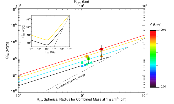
Figure 1.— Catastrophic disruption criteria $Q^{*}_{\rm{RD}}$ vs. $R_{\rm{C1}}$ (Equation (1) for $V_{\rm{i}}=$10, 20, 40, 60 km s^-1) and hydrocode results (triangles: impact parameter $b$ = 0; squares: $b$ = 0.5). Inset shows both strength- and gravity-dominated regimes for the size and velocity-dependent $Q^{*}_{\rm{RD}}$.

Figure 2.— Largest remnant mass and core mass fraction vs. scaled impact energy for head on impacts. The dotted line is Equation (2). The dashed line is Equation (3).

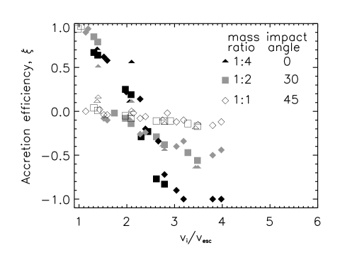
Figure 3.— Accretion efficiency $\xi$ (Equation (4)) vs. scaled impact velocity. The symbol denotes the mass ratio and the shading denotes the impact angle.

Figure 4.— Core mass fraction of the largest remnant vs. scaled impact energy for head on impacts. Panel (a) is for ice-rock bodies and panel (b) is for rock-iron bodies (Marcus et al., 2009). The dashed line is the prediction of model 1 (Equation (5)). The dash-dotted curve is the prediction of model 2 (Equations (6) and (7)). The circles are simulation results.

References

- Agnor & Asphaug (2004) Agnor, C., & Asphaug, E. 2004, ApJ, 613, L157
- Asphaug (2009) Asphaug, E. 2009, Annual Review of Earth and Planetary Sciences, 37, 413
- Benz et al. (2007) Benz, W., Anic, A., Horner, J., & Whitby, J. A. 2007, Space Science Reviews, 132, 189
- Benz et al. (1988) Benz, W., Slattery, W. L., & Cameron, A. G. W. 1988, Icarus, 74, 516
- Borucki et al. (2009) Borucki, W., et al. 2009, in IAU Symposium, Vol. 253, IAU Symposium, 289–299
- Borucki & for the Kepler Team (2010) Borucki, W. J., & for the Kepler Team. 2010, ArXiv e-prints
- Brookshaw (1998) Brookshaw, L. 1998, Working Paper Series SC-MC-9813, Faculty of Sciences (University of Southern Queensland, Australia)
- Brown et al. (2007) Brown, M. E., Barkume, K. M., Ragozzine, D., & Schaller, E. L. 2007, Nature, 446, 294
- Canup (2004) Canup, R. M. 2004, Icarus, 168, 433
- Canup et al. (2001) Canup, R. M., Ward, W. R., & Cameron, A. G. W. 2001, Icarus, 150, 288
- Charbonneau et al. (2009) Charbonneau, D., et al. 2009, Nature, 462, 891
- Figueira et al. (2009) Figueira, P., Pont, F., Mordasini, C., Alibert, Y., Georgy, C., & Benz, W. 2009, A&A, 493, 671
- Fortney et al. (2007) Fortney, J. J., Marley, M. S., & Barnes, J. W. 2007, ApJ, 659, 1661
- Fu et al. (2010) Fu, R., O’Connell, R. J., & Sasselov, D. D. 2010, ApJ, 708, 1326
- Guillot (1999) Guillot, T. 1999, Science, 286, 72
- Ida & Lin (2004) Ida, S., & Lin, D. N. C. 2004, ApJ, 604, 388
- Léger et al. (2009) Léger, A., et al. 2009, A&A, 506, 287
- Leinhardt et al. (2010) Leinhardt, Z. M., Marcus, R. A., & Stewart, S. T. 2010, ApJ, 714, 1789
- Leinhardt & Stewart (2009) Leinhardt, Z. M., & Stewart, S. T. 2009, Icarus, 199, 542
- Marcus et al. (2010) Marcus, R. A., Sasselov, D., Hernquist, L., & Stewart, S. T. 2010, ApJ, 712, L73
- Marcus et al. (2009) Marcus, R. A., Stewart, S. T., Sasselov, D., & Hernquist, L. 2009, ApJ, 700, L118
- McKinnon et al. (2008) McKinnon, W. B., Prialnik, D., Stern, S. A., & Coradini, A. 2008, Structure and Evolution of Kuiper Belt Objects and Dwarf Planets, ed. B. H. C. D. P. . M. A. Barucci, M. A., 213–241
- Miller-Ricci et al. (2009) Miller-Ricci, E., Seager, S., & Sasselov, D. 2009, ApJ, 690, 1056
- Mordasini et al. (2009) Mordasini, C., Alibert, Y., & Benz, W. 2009, A&A, 501, 1139
- Queloz et al. (2009) Queloz, D., et al. 2009, A&A, 506, 303
- Raymond et al. (2006) Raymond, S. N., Quinn, T., & Lunine, J. I. 2006, Icarus, 183, 265
- Seager et al. (2007) Seager, S., Kuchner, M., Hier-Majumder, C. A., & Militzer, B. 2007, ApJ, 669, 1279
- Senft & Stewart (2008) Senft, L. E., & Stewart, S. T. 2008, MAPS, 43, 1993
- Springel (2005) Springel, V. 2005, MNRAS, 364, 1105