Shy couplings, $\operatorname{CAT}(0)$ spaces, and the lion and man

Abstract

Two random processes $X$ and $Y$ on a metric space are said to be $\varepsilon$-shy coupled if there is positive probability of them staying at least a positive distance $\varepsilon$ apart from each other forever. Interest in the literature centres on nonexistence results subject to topological and geometric conditions; motivation arises from the desire to gain a better understanding of probabilistic coupling. Previous nonexistence results for co-adapted shy coupling of reflected Brownian motion required convexity conditions; we remove these conditions by showing the nonexistence of shy co-adapted couplings of reflecting Brownian motion in any bounded $\operatorname{CAT}({0})$ domain with boundary satisfying uniform exterior sphere and interior cone conditions, for example, simply-connected bounded planar domains with $C^{2}$ boundary.

The proof uses a Cameron–Martin–Girsanov argument, together with a continuity property of the Skorokhod transformation and properties of the intrinsic metric of the domain. To this end, a generalization of Gauss’ lemma is established that shows differentiability of the intrinsic distance function for closures of $\operatorname{CAT}({0})$ domains with boundaries satisfying uniform exterior sphere and interior cone conditions. By this means, the shy coupling question is converted into a Lion and Man pursuit–evasion problem.

T1Supported in part by NSF Grants CCF-07-29537 and DMS-09-06743, and by Grant N N201 397137, MNiSW, Poland.

, and

1 Introduction.

1.1 Results and motivation.

Benjamini, Burdzy and Chen (2007) introduced the notion of shy coupling: a coupling of Brownian motions $X$ and $Y$ (more generally, of two random processes $X$ and $Y$ on a metric space) is said to be shy if there is an $\varepsilon>0$ such that $\mathbb{P}[\operatorname{dist}(X(t),Y(t))\geq\varepsilon\mbox{ for all }t]>0$. For example consider Brownian motion $X$ on the circle: if $Y$ is produced from $X$ by a nontrivial rotation then $X$ and $Y$ exhibit a shy coupling, since $\operatorname{dist}(X,Y)$ is then constant. Interest in the existence or nonexistence of such couplings arises from the study of couplings of reflected Brownian motions, which occur in various contexts. Benjamini, Burdzy and Chen (2007) discussed existence and nonexistence of shy couplings for Brownian motions on graphs and for reflected Brownian motions in domains (connected open subsets of Euclidean space) satisfying suitable boundary regularity conditions. They restricted attention to Markovian couplings and we will do essentially the same, by restricting attention to co-adapted couplings. (This is only slightly more general, but is more convenient for expression in terms of stochastic calculus.) In particular the results in Benjamini, Burdzy and Chen (2007) showed that no shy co-adapted couplings can exist for reflected Brownian motion in convex bounded planar domains with $C^{2}$ boundary satisfying a strict convexity condition (namely, that the boundary contains no line segments). Their argument used a large deviations argument bearing some resemblance to methods from differential game theory. Kendall (2009) showed that neither differentiability nor strict convexity is required for the planar result, and also generalized the result to convex bounded domains in higher dimensions whose boundaries need no longer be smooth but still satisfy the regularity condition requiring triviality of all line segments contained in the boundary. These more recent results are based on direct proofs using ideas from stochastic control.

The work described below both generalizes the above results and also shows that absence of shyness is not confined to the case of convexity. We consider a bounded domain with boundary satisfying uniform exterior sphere and interior cone conditions and that satisfies a $\operatorname{CAT}({0})$ condition (see Definition 4) when furnished with the intrinsic metric, and we show that such domains cannot support shy co-adapted couplings of reflected Brownian motions. We do this by establishing a rather direct connection between (the nonexistence of) Brownian shy co-adapted couplings and deterministic pursuit–evasion problems. As part of this process, we generalize Gauss’ lemma (on the differentiability of the distance function) to the case of closures of $\operatorname{CAT}({0})$ domains furnished with the intrinsic metric and satisfying uniform exterior sphere and interior cone conditions. It may not be evident to the reader exactly how the stochastic and undirected notion of Brownian motion can be connected to the deterministic and intentional notion of a pursuit–evasion problem, and it was not initially evident to us [though, in retrospect, this is latent in Benjamini, Burdzy and Chen (2007)], but nonetheless the connection is both immediate and useful.

The pursuit–evasion problem in question is a well-known problem concerning a Lion chasing a Man in a disk, both travelling at unit speed: R. Rado’s celebrated “Lion and Man” problem. Our shy coupling problem leads us to consider the generalization in which the Lion chases the Man in a bounded domain which is $\operatorname{CAT}({0})$ in its intrinsic metric. Isaacs (1965) is the classic reference for pursuit–evasion problems; Nahin (2007) provides an accessible exposition of the special case of the Lion and Man problem in the unit disk. Littlewood [(1986), pages 114–117 in Bollobas’ extended edition] provides a brief description of the Lion and Man problem with an indication of its history, including a presentation of Besicovitch’s celebrated proof that in the disc the Man can evade the Lion indefinitely, even though the distance between Lion and Man may tend to zero. A generalization of discrete-time pursuit–evasion to bounded $\operatorname{CAT}({0})$ domains is dealt with in Alexander, Bishop and Ghrist (2006); we summarize concepts from metric geometry and develop results required for the continuous-time variant in Section 2, and it is here that we generalize the Gauss lemma to the case of closures of $\operatorname{CAT}({0})$ domains with sufficient boundary regularity (Proposition 14).

In particular, Section 2 rigorously develops the geometric results required to reason with these concepts in the context of the intrinsic metric for the domain $D$ (determined by lengths of paths restricted to lie within $D$). On a first reading one should feel free to note only the general ideas of Section 2, and then to pass quickly on to the probabilistic arguments in the remaining sections of the paper.

In Section 3, we describe how continuous-time pursuit–evasion problems can be solved in $\operatorname{CAT}({0})$ domains. We obtain an upper bound for the time of $\varepsilon$-capture, expressed in terms of domain geometry. Simultaneously with and independently of our research project, Chanyoung Jun developed in his Ph.D. thesis [Jun (2011)] a theory of continuous pursuit in $\operatorname{CAT}({\kappa})$ spaces that overlaps somewhat with our results.

Pursuit–evasion games involve control of the velocity of the pursuer so as to bring it arbitrarily close to the evader, regardless of what strategy may be adopted by the evader. In order to show nonexistence of Brownian shy couplings, we investigate the possibility of bringing the Brownian pursuer (the Brownian Lion) arbitrarily close to the Brownian evader (the Brownian Man), regardless of how the Brownian motion of the Brownian Man is coupled to that of the Brownian Lion. The connection between coupling and deterministic Lion and Man problems is described in Section 4: a suitable pursuit strategy generates a vector field $\chi$ on the configuration manifold generated by the locations of Brownian Lion and Man. (More pedantically, it generates a section of the pullback of the tangent bundle of $D$ to the configuration space of the pursuer and evader before capture.) If this pursuit strategy can be guaranteed to bring the Lion within $\varepsilon/2$ of Man by a bounded time $t_{c}$ in the deterministic problem, then a Cameron–Martin–Girsanov argument together with a continuity property for the Skorokhod transformation shows that the Brownian Lion has a positive probability of getting within distance $\varepsilon$ of the Brownian Man, whatever coupling strategy might be adopted by the Brownian Man.

The paper concludes with Section 5, which discusses possible extensions of these results, further questions, and conjectures.

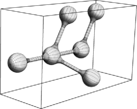
Figure 1: A $\operatorname{CAT}({0})$ example which is the union of five dumbbells.

We now state the main results of this paper, using terms defined in Section 2. Here and elsewhere in the paper, we consider only domains in Euclidean space of dimensions $2$ or higher.

Theorem 1

Suppose that $D$ is a bounded domain with boundary satisfying uniform exterior sphere and interior cone conditions, and which is $\operatorname{CAT}({0})$ in its intrinsic metric. There can be no shy co-adapted coupling for reflected Brownian motion in $D$.

Examples of $\operatorname{CAT}({0})$ domains include convex domains and domains that are the unions of a pair of convex domains. See, for instance, Bridson and Haefliger (1999) and Alexander, Bishop and Ghrist (2006), where more general examples are also provided; in particular, a large range of examples follows from iterated application of the result that if two $\operatorname{CAT}({0})$ domains have a geodesically convex intersection then their union is $\operatorname{CAT}({0})$. The exterior sphere and interior cone conditions in the theorem are required in order to apply the results of Saisho (1987) to generate reflected diffusions using the Skorokhod transformation.

The three-dimensional domain in Figure 1 is $\operatorname{CAT}({0})$. There are two different ways to see this. First, it is easy to see that for every point on the boundary of the domain, at most one of the principal curvatures is negative. An alternative way to see that the domain is $\operatorname{CAT}({0})$ is to observe that a single dumbbell (the union of two spheres and the connecting tube) is a $\operatorname{CAT}({0})$ domain. The whole set is the union of five dumbbells. The nonempty intersections of the dumbbells are balls.

Remarkably, all bounded simply-connected planar domains are $\operatorname{CAT}({0})$ in their intrinsic metrics. Thus, in the planar case, there is an immediate consequence of Theorem 1 which is a strikingly powerful result depending principally on topological conditions:

Theorem 2

Suppose that $D$ is a simply-connected bounded planar domain with boundary satisfying uniform exterior sphere and interior cone conditions. There can be no shy co-adapted coupling for reflected Brownian motion in $D$.

1.2 Some basic tools for probabilistic coupling.

All probabilistic couplings considered here are co-adapted couplings, which are defined for general Markov processes in Kendall (2009). In essence, a co-adapted coupling of two Markov processes is a construction of the two Markov processes on the same probability space, which are adapted to the same filtration such that each process possesses the prescribed transition functions with respect to the common filtration.

In this paper, it suffices to work with co-adapted couplings of $d$-dimensional Brownian motions: $B$ and $\widetilde{B}$ are said to be co-adaptively coupled Brownian motions if they are defined on the same probability space and adapted to the same filtration $\{\mathcal{F}_{t}\dvtx t\geq 0\}$ and if, in addition, both satisfy an independent increments property taken with respect to the common filtration:

$$B_{t+s}-B_{t}\mbox{ is independent of }\mathcal{F}_{t}\mbox{ for all }t,s\geq 0,$$

$$\widetilde{B}_{t+s}-\widetilde{B}_{t}\mbox{ is independent of }\mathcal{F}_{t}\mbox{ for all }t,s\geq 0.$$

Note that $B_{t+s}-B_{t}$ and $\widetilde{B}_{t+s}-\widetilde{B}_{t}$ need not be independent of each other. Kendall [(2009), Lemma 6] shows that one may represent such a coupling using stochastic calculus, possibly at the cost of augmenting the filtration by adding a further independent Brownian motion $C$: there exist $(d\times d)$-matrix-valued predictable random processes $\mathbb{J}$ and $\mathbb{K}$ such that

$$\widetilde{B}=\int\mathbb{J}^{\top}\,\mathrm{d}B+\int\mathbb{K}^{\top}\,\mathrm{d}C;$$

moreover, one may choose $\mathbb{J}^{\top}\mathbb{J}+\mathbb{K}^{\top}\mathbb{K}$ to be equal to the $(d\times d)$ identity matrix at all times.

A pair of processes $X$ and $\widetilde{X}$ is said to form a co-adapted coupling if they can be defined by strong solutions of stochastic differential equations driven by $B$, $\widetilde{B}$, respectively. In the paper, we will employ the stochastic differential equation obtained from the Skorokhod transformation for reflected Brownian motion in a domain $D$ of suitable boundary regularity, such as under uniform exterior sphere and uniform interior cone conditions, as discussed in Section 2. For $r>0$, set $\mathcal{N}_{x,r}=\{\nu\in\mathbb{R}^{d}\dvtx|\nu|=1,\mathcal{B}(x+r\nu,r)\cap D=\varnothing\}$. The vectors $\nu$ can be be viewed as “exterior normal unit vectors at $x\in\partial D$”; note that there may be more than one such vector at a particular point $x\in\partial D$. The set $\mathcal{N}_{x,r}$ is decreasing in $r$, and the uniform exterior sphere condition asserts that $r$ can be chosen so that, for all $x\in\partial D$, $\mathcal{N}_{x,r}\neq\varnothing$, with $\mathcal{N}_{x,r}=\mathcal{N}_{x,s}$ for $0<s\leq r$. Under uniform exterior sphere and uniform interior cone conditions, Saisho (1987) has shown that, given a driving Brownian motion $B$, there exists a unique solution pair $(X,L^{X})$ satisfying

$$\mathrm{d}X=\mathrm{d}B-\nu_{X}\,\mathrm{d}L^{X},$$

$$L^{X}\mbox{ is nondecreasing and increases only when }X\in\partial D,$$

$$\nu_{X}\in\mathcal{N}_{X,r}.$$

Thus $L^{X}$ may be viewed as the local time of the reflected Brownian motion $X$ on the boundary $\partial D$.

In this paper, all vectors are assumed to be column vectors unless specified otherwise.

2 $\operatorname{CAT}({0})$ geometry and the deterministic pursuit–evasion problem.

Recall that the intrinsic metric for a domain $D$ is generated by the infimum of Euclidean lengths $\operatorname{len}(\gamma)$ of smooth connecting paths $\gamma$ lying wholly within the domain. (The definition is typically formulated in the context of general metric spaces and regularizable paths.)

Definition 3.

The intrinsic distance between two points $x$ and $y$ in a domain $D$ is given by

$$\operatorname{dist}_{\mathrm{intr}}(x,y)=\inf\{\operatorname{len}(\gamma)\dvtx\gamma\mbox{ is a smooth path connecting }x\mbox{ and }y\mbox{ in }D\}.$$ (1)

For a domain $D$, a standard compactness argument shows that paths attaining the infimum of (1) will always exist in the closure of the domain: these are called intrinsic geodesics.

As described in Bridson and Haefliger [(1999), Section II.1, Definition 1.1] [see also Burago, Burago and Ivanov (2001)], one can define simple curvature conditions for metric spaces such as $(D,\operatorname{dist}_{\mathrm{intr}})$, based on the behaviour of geodesic triangles. We first give the case of comparison with flat Euclidean space (which has zero curvature).

Definition 4.

We say that $(D,\operatorname{dist}_{\mathrm{intr}})$ is a $\operatorname{CAT}({0})$ domain if the following triangle comparison holds: Suppose that $\Gamma_{a,b}$, $\Gamma_{a,c}$ and $\Gamma_{b,c}$ are unit-speed intrinsic geodesics for $D$, connecting points $a$ to $b$, $a$ to $c$ and $b$ to $c$, respectively. Then, for all such geodesic triangles,

$$\operatorname{dist}_{\mathrm{intr}}(\Gamma_{a,b}(s),\Gamma_{a,c}(t))\leq r(s,t),$$

where $r(s,t)$ is the distance between points at distance $s$, respectively, $t$, from $\widetilde{a}$ along the side $\widetilde{a}\widetilde{b}$, respectively, $\widetilde{a}\widetilde{c}$, of an ordinary Euclidean triangle $\widetilde{a}\widetilde{b}\widetilde{c}$ that has the same side lengths.

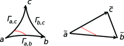
Figure 2: Illustration of the $\operatorname{CAT}({0})$ condition.

Consequently, chords of triangles in $(D,\operatorname{dist}_{\mathrm{intr}})$ are shorter than comparable chords of the comparable Euclidean triangles, as illustrated in Figure 2.

Bridson and Haefliger [(1999), Section II.1, Definition 1.1] actually introduces the more general notion of a $\operatorname{CAT}({\kappa})$ domain [see also Alexander, Bishop and Ghrist (2010), Appendix A]. Here we describe the case when comparisons are drawn with triangles on a sphere of radius $1/\sqrt{\kappa}$, for $\kappa>0$ (hence the sphere has curvature $\kappa$). It is necessary here to restrict attention to suitably small triangles, as measured by perimeter.

Definition 5.

We say that $D$ is a $\operatorname{CAT}({\kappa})$ domain for $\kappa>0$ if any two distinct points with distance less than $\pi/\sqrt{\kappa}$ are joined by a geodesic and the distance between any two points of any geodesic triangle $\triangle pqr$ of perimeter less than $2\pi/\sqrt{\kappa}$ is no greater than the distance between the corresponding points of the model triangle $\triangle\widetilde{p}\widetilde{q}\widetilde{r}$ with the same sidelengths in the 2-dimensional Euclidean sphere of radius $1/\sqrt{\kappa}$.

Gromov introduced the acronym $\operatorname{CAT}$, standing for Cartan, Aleksandrov, Toponogov. In this paper, we will mostly consider spaces $\operatorname{CAT}({\kappa})$ with $\kappa=0$. We include some results concerning the $\operatorname{CAT}({\kappa})$ case with $\kappa>0$ because they will be used in the forthcoming paper Bramson, Burdzy and Kendall (2011).

As noted in Bridson and Haefliger [(1999), Proposition II.3.1] [see also Burago, Burago and Ivanov (2001), Section 4.3], in $\operatorname{CAT}({\kappa})$ spaces the notion of angle is well-defined for (locally) minimal geodesics.

Consequently, geodesics in a $\operatorname{CAT}({0})$ space diverge at most as fast as corresponding geodesics in Euclidean space. Note that $\operatorname{CAT}({0})$ is a global condition, applying to all possible geodesic triangles. In particular it can be shown that $\operatorname{CAT}({0})$ spaces are always simply-connected and indeed contractible [Bridson and Haefliger (1999), Proposition II.1.4, or Alexander, Bishop and Ghrist (2010), Appendix A].

Remarkably, bounded planar domains are $\operatorname{CAT}({0})$ if they are simply-connected; see Bishop (2008) for a careful proof. Readers may convince themselves of this at an intuitive level by drawing pictures (as exemplified in Figure 3); as is the case with other foundational results in metric spaces, the rigorous proof requires delicate reasoning.

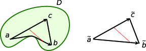
Figure 3: Illustration of the $\operatorname{CAT}({0})$ property for a bounded simply-connected planar domain. The effect of the boundary is to make the triangle “skinnier” than its Euclidean counterpart, thus establishing the $\operatorname{CAT}({0})$ comparison property.

We now introduce two complementary notions of boundary regularity following Saisho (1987). An exterior sphere condition (also called weak convexity) requires that every boundary point is touched by at least one external sphere. Here and in the following, let $\mathcal{B}(y,s)$ denote the open Euclidean ball of radius $s$ centered on $y$.

Definition 6 ([Uniform exterior sphere condition, from Saisho (1987), Section 1, Condition $(A)$]).

A domain $D$ is said to satisfy a uniform exterior sphere condition, based on radius $r$ if, for every $x\in\partial D$, the set of “exterior normals” $\mathcal{N}_{x,r}=\{\nu\in\mathbb{R}^{d}\dvtx|\nu|=1,\mathcal{B}(x+r\nu,r)\cap D=\varnothing\}$ is nonempty, with $\mathcal{N}_{x,r}=\mathcal{N}_{x,s}$ for $0<s\leq r$.

Thus a uniform exterior sphere condition allows one to move a fixed ball all the way around the outside of the domain boundary. In particular, $D$ can have no “inward-pointing corners”. Here is a simple observation which will be useful later and corresponds to the intuition about being able to move a fixed ball about $D$; such $D$ may be represented as intersections of complements of balls, in a manner entirely analogous to the representation of a convex set as the intersection of half-planes (so justifying the alternative term “weak convexity”).

Lemma 7

Suppose that the domain $D$ satisfies a uniform exterior sphere condition based on radius $r$. Then

$$\overline{D}=\bigcap\{\mathcal{B}(z,r)^{c}\dvtx\mathcal{B}(z,r)\cap D=\varnothing\}.$$

Let the Minkowski sum $A\oplus B$ of two Euclidean sets $A$ and $B$ be $A\oplus B=\{x+y\dvtx x\in A,y\in B\}$. Certainly $F=\bigcap\{\mathcal{B}(z,r)^{c}\dvtx\mathcal{B}(z,r)\cap D=\varnothing\}$ is closed, since $\mathcal{B}(z,r)$ is an open ball. Moreover $D\subseteq F$; hence $\overline{D}\subseteq F$. Furthermore $F\subseteq\overline{D}\oplus\mathcal{B}(\mathbf{o},r)$, where $\mathbf{o}$ is the origin of the ambient Euclidean space.

Following Saisho [(1987), Remark 1.3], because of the uniform exterior sphere condition, we can define a projection $x\mapsto\overline{x}$ from $\overline{D}\oplus\mathcal{B}(\mathbf{o},r)$ onto $\overline{D}$ using the Euclidean metric. Consider $x\in\overline{D}\oplus\mathcal{B}(\mathbf{o},r)$. Then the projection $\overline{x}\in\overline{D}$ is defined; moreover, if $\overline{x}\in\partial D$ and $x\notin\overline{D}$, then

$$\frac{\overline{x}-x}{|\overline{x}-x|}\in\mathcal{N}_{\overline{x},r}$$

is a unit vector whose offset produces a tangent sphere of radius $r$ at $\overline{x}$ [using the argument of Saisho (1987)]. But this implies that if $x\in(\overline{D}\oplus\mathcal{B}(\mathbf{o},r))\setminus D$ then

$$x\in\mathcal{B}\biggl{(}\overline{x}-r\frac{\overline{x}-x}{|\overline{x}-x|},r\biggr{)}$$

and so $x\notin F$. Accordingly $\overline{D}=F$ as required.

On the other hand, a uniform interior cone condition requires that any boundary point supports a bounded cone truncated to the boundary of a ball, and moreover that the cone may be translated locally within the domain.

Definition 8 ([Uniform interior cone condition, from Saisho (1987), Section 1, Condition $(B^{\prime})$]).

A domain $D$ is said to satisfy a uniform interior cone condition, based on radius $\delta>0$ and angle $\alpha\in(0,\pi/2]$, if, for every $x\in\partial D$, there is at least one unit vector $\mathbf{m}$ such that the cone $C(\mathbf{m})=\{z\dvtx\langle z,\mathbf{m}\rangle>|z|\cos\alpha\}$ satisfies

$$\bigl{(}y+C(\mathbf{m})\bigr{)}\cap\mathcal{B}(x,\delta)\subseteq D\qquad\mbox{for all }y\in D\cap\mathcal{B}(x,\delta).$$

We say that the cone $y+C(\mathbf{m})$ is based on $y$ and angle $\alpha\in(0,\pi/2]$.

Thus a uniform interior cone condition implies that the “outward-pointing corners” must not be too sharp. Note that Saisho actually uses a slightly weaker condition with less intuitive content [Saisho (1987), Condition $(B)$]; we do not consider this weaker notion further in what follows.

In fact, the property of a domain satisfying a uniform interior cone condition is equivalent to it being a Lipschitz domain.

Definition 9 ((Lipschitz domain)).

Recall that a function $f\dvtx\mathbb{R}^{d-1}\to\mathbb{R}$ is Lipschitz, with constant $\lambda<\infty$, if $|f(x)-f(y)|\leq\lambda|x-y|$ for all $x,y\in\mathbb{R}^{d-1}$. A domain $D$ is said to be Lipschitz, with constant $\lambda$, if there exists $\delta>0$ such that, for every $x\in\partial D$, there exists an orthonormal basis $e_{1},e_{2},\ldots,e_{d}$ and a Lipschitz function $f\dvtx\mathbb{R}^{d-1}\to\mathbb{R}$, with constant $\lambda$, such that

$$\mathcal{B}(x,\delta)\cap D=\{y\in\mathcal{B}(x,\delta)\dvtx f(y_{1},\ldots,y_{d-1})<y_{d}\},$$

where we write $y_{1}=\langle y,e_{1}\rangle,\ldots,y_{d}=\langle y,e_{d}\rangle$.

The equivalence of Definitions 8 and 9 depends on the fact that the cone axis vector in Definition 8 is chosen to be the same for all $y\in\mathcal{B}(x,\delta)$, and so can be used as $e_{d}$ in the orthonormal basis for $\mathcal{B}(x,\delta)$ required in Definition 9. The constants $\lambda$ and $\alpha$ in Definitions 8 and 9 are related by $\lambda=\cot\alpha$, while the two $\delta$’s of Definitions 8 and 9 may be taken to be equal. Note too that if the uniform interior cone/Lipschitz domain property holds for a given $\delta>0$, then evidently it also holds for all smaller $\delta$.

If a domain satisfies a uniform interior cone condition, then the intrinsic metric and Euclidean metric properties are closely related.

Lemma 10

A domain $D$ that is bounded in Euclidean metric and satisfies a uniform interior cone condition must have finite intrinsic diameter.

Certainly $\operatorname{dist}_{\mathrm{intr}}(x,y)$ is a continuous function of $(x,y)$ in the open set $D\times D$ and takes only finite values there. Note that the domain $D$ is path-connected, being an open connected subset of Euclidean space.

Suppose that $D$ satisfies a uniform interior cone condition based on radius $\delta>0$ and angle $\alpha\in(0,\pi/2]$. If m is a unit vector for the interior cone condition at $x\in\partial D$ then geometrical arguments show that $x+\frac{1}{2}\delta\textbf{m}$ is at least $\frac{1}{2}\delta\sin\alpha$ from the exterior $D^{c}$. Choosing $\delta^{\prime}$ with $0<\delta^{\prime}<\frac{1}{2}\delta\sin\alpha$, it follows that any such $x+\frac{1}{2}\delta\textbf{m}$ belongs to

$$D\ominus\mathcal{B}(\mathbf{o},\delta^{\prime})\stackrel{{\scriptstyle\mathrm{def}}}{{=}}\bigl{(}D^{c}\oplus\mathcal{B}(\mathbf{o},\delta^{\prime})\bigr{)}^{c}=\{x\in D\dvtx{\mathcal{B}(x,\delta^{\prime})}\subset D\},$$

which itself is closed. Inheriting boundedness from $D$, it is therefore compact in the Euclidean topology, and hence also in the topology derived from the intrinsic metric, since the two metrics are locally equal away from the boundary of $D$. Hence $\{\operatorname{dist}_{\mathrm{intr}}(x,y)\dvtx x,y\in D\ominus\mathcal{B}(\mathbf{o},\delta^{\prime})\}$ attains a maximum value, which is therefore finite. However, for any $x^{\prime},y^{\prime}\in D$, we have

$$\operatorname{dist}_{\mathrm{intr}}(x^{\prime},y^{\prime})\leq\delta+\sup\{\operatorname{dist}_{\mathrm{intr}}(x,y)\dvtx x,y\in D\ominus\mathcal{B}(\mathbf{o},\delta^{\prime})\},$$ (2)

because we have used the uniform interior cone condition to ensure that from each point on the boundary there is a straight-line segment of length $\frac{1}{2}\delta$ to $\{\operatorname{dist}_{\mathrm{intr}}(x,y)\dvtx x,y\in D\ominus\mathcal{B}(\mathbf{o},\delta^{\prime})\}$. Hence the intrinsic diameter must be bounded by the right-hand side of (2).

The full force of the uniform interior cone condition is not required for the above result; the proof does not require coordination of the directions of interior cones at different base-points. The full force of the uniform interior cone condition assures us that any path of finite length leading in $D$ to a point $x$ on the boundary of $D$ can be deformed continuously in $D$ into one which in its final phase is the segment on which the interior cone at $x$ is based. Moreover, the lengths of the curves throughout this deformation can be constrained to be arbitrarily close to the length of the original path. This allows us to view $D$ as a topological manifold with boundary, which is continuously embedded in the ambient Euclidean space. More than this, it shows that the completion $\hat{D}$ of $D$ under the intrinsic metric can be identified with the Euclidean closure $\overline{D}$ and moreover that the intrinsic metric and the Euclidean metric actually endow $\overline{D}$ with the same topology. Finally, Bridson and Haefliger [(1999), Corollary II.3.11] show that the closure $\overline{D}$, viewed as the completion $\hat{D}$ of $D$ in intrinsic metric, inherits $\operatorname{CAT}({0})$ structure from $D$.

2.1 Regularity for geodesics.

We wish to consider pursuit–evasion in a bounded $\operatorname{CAT}({0})$ domain. Lion and Man both move with unit speed, with the Lion seeking to draw closer to the Man by using a “greedy” pursuit strategy (which is not necessarily optimal). This Lion strategy can be phrased in terms of an $\mathbb{R}^{d}$-valued field $\chi$ of unit vectors defined on the configuration space $(\overline{D}\times\overline{D})\setminus\{(x,x)\dvtx x\in\overline{D}\}$, such that $\chi(x,y)$ is the initial velocity of the unit-speed geodesic moving from $x$ to $y$. (This is the vector field described pedantically in Section 1 as a section of the pullback of the tangent bundle of $D$ to the configuration space of the pursuer and evader before capture.)

We first show that the combination of uniform exterior sphere and uniform interior cone/Lipschitz conditions implies that, working locally, every boundary point of the intersection of the domain $D$ with a suitable $2$-plane will support an exterior sphere, albeit with smaller radius.

Lemma 11

Suppose that $D$ is a domain satisfying a uniform exterior sphere condition based on radius $r>0$, and a uniform interior cone condition based on radius $\delta>0$ and angle $\alpha\in(0,\pi/2]$. Suppose that $z\in\partial D$ and $e_{d}$ is the $d$th vector in the orthonormal basis corresponding to $z$ as in Definition 9. Let $P$ be a $2$-plane intersecting $D$ and containing $z$ and $z+e_{d}$. Then there exists $w\in P$, with $|w-z|=\operatorname{dist}(w,D\cap P)=r\sin\alpha$ and $\mathcal{B}(w,r\sin\alpha)\cap(D\cap P)=\varnothing$.

Since the interior cone condition is uniform, the lemma shows that every point in the boundary of $D\cap P$ near $z$ must support an exterior sphere of radius $r\sin\alpha$.

Figure 4: Illustration of interior cone $C_{z}$ and exterior ball $\mathcal{B}(y,r)$ at $z\in D$.

Proof of Lemma 11 Suppose that $z\in\partial D$ with $e_{d}$ defined as above. Let $P$ be a $2$-plane containing $z$ and $z+e_{d}$. Since $z\in\partial D$, there is an exterior sphere touching $z$, defined by a ball $\mathcal{B}(y,r)\subseteq D^{c}$ with $z\in\overline{\mathcal{B}(y,r)}$. By Definition 9, the cone

$$C_{z}=\{w\dvtx\langle w-z,e_{d}\rangle>|w-z|\cos\alpha\}$$

lies locally in $D$, in the sense that $C_{z}\cap\mathcal{B}(z,\delta)\subseteq D$ (see Figure 4). If $\frac{\pi}{2}+\beta$ is the angle between $e_{d}$ and $y-z$, then two-dimensional geometry (Figure 5) shows that

$$\min\{|y-(\gamma e_{d}+z)|\dvtx\gamma\in\mathbb{R}\}=r\cos\beta.$$

But $\beta\geq\alpha$ if $C_{z}\cap\mathcal{B}(z,\delta)\subseteq D$ and $\mathcal{B}(y,r)\subseteq D^{c}$; moreover, the line $\{\gamma e_{d}+z\dvtx\gamma\in\mathbb{R}\}$ must lie in $P$. Hence the distance from $y$ to $P$ is at most $r\cos\beta\leq r\cos\alpha$. Consequently the radius of the disk $\mathcal{B}(y,r)\cap P$ is at least $r\sin\alpha$; since $z\in\partial(D\cap P)$ and $\mathcal{B}(y,r)\cap P$ is an exterior sphere to $z$ in $P$, the lemma follows.

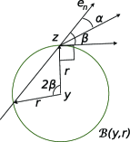
Figure 5: Two-dimensional section of Figure 4 illustrating the underlying two-dimensional geometry.

We can now establish some important technical consequences of the uniform exterior sphere and interior cone conditions together with the $\operatorname{CAT}({0})$ condition; namely, that the Euclidean and intrinsic distances are locally comparable, and that the vector field $\chi$ is continuous with reference to the common topology of the Euclidean metric and the intrinsic metric, and hence is uniformly continuous over regions for which the two arguments are well-separated. This is spelled out in the following proposition. In fact we state and prove a generalization of the result for $\operatorname{CAT}({\kappa})$ domains with $\kappa\geq 0$, so that we can apply it in the forthcoming paper Bramson, Burdzy and Kendall (2011).

Proposition 12

Suppose that $D$ is a $\operatorname{CAT}({\kappa})$ domain with $\kappa\geq 0$, bounded in the Euclidean metric and satisfying a uniform exterior sphere condition based on radius $r>0$, and a uniform interior cone condition based on radius $\delta>0$ and angle $\alpha\in(0,\pi/2]$. We can and will assume without loss of generality that $\lambda=\cot\alpha>1$. [(1)]

Suppose $a$, $b\in\overline{D}$ are close in the Euclidean metric, in the sense that

$$|a-b|<\min\{\delta/(4\lambda),2r\sin\alpha\}.$$ (3)

Then

$$2r\sin\alpha\sin\biggl{(}\frac{\operatorname{dist}_{\mathrm{intr}}(a,b)}{2r\sin\alpha}\biggr{)}\leq|a-b|\leq\operatorname{dist}_{\mathrm{intr}}(a,b).$$ (4)

Suppose that $\kappa=0$. Intrinsic geodesics for $D$ [necessarily minimal, by the $\operatorname{CAT}({0})$ condition] are continuously differentiable and their direction fields satisfy a Lipschitz property with constant $\frac{4}{\sqrt{3}}\frac{1}{2r\sin\alpha}$ that therefore holds uniformly for all minimal intrinsic geodesics in $D$ and hence in $\overline{D}$ [since $\operatorname{CAT}({0})$ geodesics depend continuously on their endpoints]. For $\kappa>0$, the same conclusion holds for minimal intrinsic geodesics with endpoints in $\overline{D}$ which are separated by intrinsic distance strictly less than $\pi/\sqrt{\kappa}$.

For $x$, $y$ in $\overline{D}$ with $\operatorname{dist}_{\mathrm{intr}}(x,y)<\pi/\sqrt{\kappa}$ (as usual, $\pi/\sqrt{0}=\infty$), let $\chi(x,y)$ be the unit vector at $x$ pointing along the unique intrinsic geodesic $\gamma^{(x,y)}$ from $x$ to $y$. Then $\chi(x,y)$ depends continuously on $(x,y)$ in $A=\{(x,y)\in\overline{D}\times\overline{D}\dvtx 0<\operatorname{dist}_{\mathrm{intr}}(x,y)<\pi/\sqrt{\kappa}\}$ and hence is uniformly continuous over compact subregions of $A$.

Proof of part (1) Definitions 8 and 9 are equivalent, so the domain $D$ is Lipschitz with constant $\lambda=\cot\alpha$. For each ball of radius $\delta$, we may therefore construct a coordinate system $e_{1},\ldots,e_{d}$ and a Lipschitz function $f$ to implement the Lipschitz property of $D$.

Consider $a$, $b\in\overline{D}$ with $|a-b|<\min\{\delta/(4\lambda),2r\sin\alpha\}$. If the line segment $S$ between $a$ and $b$ does not intersect $\partial D$, then it must form the (unique, minimal) intrinsic geodesic between $a$ and $b$, and (4) follows immediately. If $S$ does not intersect $\operatorname{int}(D^{c})$, then we can cover the intersection $S\cap\partial D$ with a single $\mathcal{B}(z,\delta)$ (for $z\in\partial D$) and use the unit vector $e_{d}$ corresponding to the ball (equivalently, the unit vector defining the cone for the ball) to perturb $S$ to a regularizable path in $D$ (save for the endpoints) with length arbitrarily close to that of $S$. Hence $S$ is the intrinsic geodesic between $a$ and $b$, and therefore (4) follows immediately. So we can confine our attention to the case when $a\neq b$ and $S$ intersects $\operatorname{int}(D^{c})$.

Applying Definition 9 to $\mathcal{B}(a,\delta)$, there is a Lipschitz function $f\dvtx\mathbb{R}^{d-1}\to\mathbb{R}$, with Lipschitz constant $\lambda=\cot\alpha$, and an orthonormal basis $e_{1},\ldots,e_{d}$, such that

$$\mathcal{B}(a,\delta)\cap D=\{y\in\mathcal{B}(a,\delta)\dvtx f(y_{1},\ldots,y_{d-1})<y_{d}\},$$ (5)

where $y_{1}=\langle y,e_{1}\rangle,\ldots,y_{d}=\langle y,e_{d}\rangle$. Consider

$$\mathcal{C}(a) = \{y\in\mathbb{R}^{d}\dvtx(|y_{1}-a_{1}|^{2}+\cdots+|y_{d-1}-a_{d-1}|^{2})^{1/2}<\delta/(4\lambda),$$

$$\hskip 183.0pt\phantom{\{}|y_{d}-a_{d}|<\delta/2\}$$

and note that, since $\lambda>1$, it is a consequence of (5) that $\mathcal{C}(a)\subset\mathcal{B}(a,\delta)$. Moreover $f$ has Lipschitz constant $\lambda$, so we can control the behaviour of that part of the boundary of $D$ lying within $\mathcal{C}(a)$:

$$\{y\in\mathbb{R}^{d}\dvtx(|y_{1}-a_{1}|^{2}+\cdots+|y_{d-1}-a_{d-1}|^{2})^{1/2}<\delta/(4\lambda),$$

$$\hskip 150.0pt\quad f(y_{1},\ldots,y_{d-1})=y_{d}\}$$ (6)

$$\qquad=\{y\in\mathcal{C}(a)\dvtx f(y_{1},\ldots,y_{d-1})=y_{d}\}=\partial D\cap\mathcal{C}(a).$$

Applying Lemma 11 to the $2$-plane

$$P=a+\mbox{linear span}\{b-a,e_{d}\},$$

every boundary point of $D\cap P\cap\mathcal{C}(a)$ supports an exterior disk of radius $r\sin\alpha$. [Note that the Lipschitz representation implies that $(\partial D)\cap P\cap\mathcal{C}(a)=\partial(D\cap P)\cap\mathcal{C}(a)$.] We shall use these exterior disks to construct a short path between $a$ and $b$.

It follows from (3) and (2.1) that the two rays from $a$ and $b$ along the direction $e_{d}$ must lie in $P\cap D$ until they leave $\mathcal{C}(a)$:

$$\mathcal{C}(a)\cap\{a+\gamma e_{d}\dvtx\gamma>0\} \subseteq P\cap D,$$

$$\mathcal{C}(a)\cap\{b+\gamma e_{d}\dvtx\gamma>0\} \subseteq P\cap D.$$

We set $u$, $v$ to be the intersections of these rays with $\partial\mathcal{C}(a)$. For each $\eta\in(0,1)$, consider the point $\eta a+(1-\eta)b$ and the open segment which is the intersection of the corresponding ray with $\mathcal{C}(a)$, namely

$$\mathcal{C}(a)\cap\{\eta a+(1-\eta)b+\gamma e_{d}\dvtx\gamma>0\}.$$

It follows from (3) and (2.1) that a nonempty final sub-segment

$$\mathcal{C}(a)\cap\{\eta a+(1-\eta)b+\gamma e_{d}\dvtx\gamma>\gamma_{\eta}\}$$

must lie in $D\cap P$. But then any exterior disk for $\eta a+(1-\eta)b+\gamma_{\eta}e_{d}$ has to avoid the rays defined in (2.1) as well as the above nonempty final sub-segments; it must not intersect the segments $[a,u]$ and $[b,v]$, and also may not intersect that portion of $\partial\mathcal{C}(a)$ which intersects rays $\{\eta a+(1-\eta)b+\gamma e_{d}\dvtx\gamma>0\}$ (see Figure 6). Consequently (since $|a-b|<2r\sin\alpha$) such an exterior disk must have center lying on the side of the line through $a$ and $b$ which is opposite to the side containing $u$ and $v$, and must not intersect the complement of the segment $S$ in the line through $a$ and $b$.

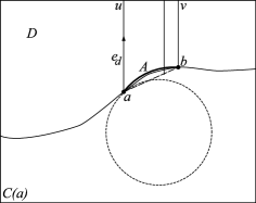
Figure 6: Illustration of proof of Proposition 12, part (1). The aspect ratio is not realistic—the height of $\mathcal{C}(a)$ must be at least twice its horizontal diameter.

The envelope of the boundaries of all such disks of radius $r\sin\alpha$ in $D\cap P$ is formed by the complement of the segment $S$ in the line through $a$ and $b$ together with the minor arc $A$ of the circle of radius $r\sin\alpha$ running through $a$ and $b$. We can use $A$ to generate a short path between $a$ and $b$ in $\overline{D}$ as follows. If $A$ does not intersect one of the rays in (2.1) then $A$ itself suffices; otherwise a still shorter path may be formed which lies wholly in $\overline{D}$ by making a short-cut using the relevant ray. In any case a small perturbation of $A$ or the short-cut version, using the vector $e_{d}$, will provide a path in $D$ from $a$ to $b$ of length less than the length of $A$ plus an arbitrarily small increment. Calculation of the length of the minor arc $A$ now leads to the desired bounds on $\operatorname{dist}_{\mathrm{intr}}(a,b)$ as given in (4).

Proof of part (2) Consider points $a,b$ and $c$ in $\overline{D}$, lying in this order along an intrinsic geodesic $\Gamma$ in $\overline{D}$. We will need the geodesic $\Gamma$ to be minimal. This is immediate in case $\kappa=0$; in the case $\kappa>0$ it follows if we require that the length of $\Gamma$ is strictly less than $\pi/\sqrt{\kappa}$. For some positive $t<\min\{\delta/(4\lambda),2r\sin\alpha\}$, suppose that the intrinsic distances between $a$ and $b$ and between $b$ and $c$ are both equal to $t$. Since $\Gamma$ is a minimal geodesic, the intrinsic distance between $a$ and $c$ must be $2t$. Let $\rho_{1}=|a-b|$, $\rho_{2}=|b-c|$ and $\rho_{3}=|a-c|$ be the Euclidean distances between these three pairs of points and let $\pi-\theta$ be the interior angle at $b$ in the Euclidean triangle $abc$. By the cosine formula,

$$\cos\theta=-\cos(\pi-\theta)=-\frac{\rho_{1}^{2}+\rho_{2}^{2}-\rho_{3}^{2}}{2\rho_{1}\rho_{2}}=\frac{\rho_{3}^{2}-\rho_{1}^{2}-\rho_{2}^{2}}{2\rho_{1}\rho_{2}}.$$

The upper bound on $t$ means we can apply (4) to the intrinsic and Euclidean distances between $a$, $b$ and $c$. Hence $\rho_{1}\leq t$, $\rho_{2}\leq t$ and

$$\rho_{3}\geq 2r\sin\alpha\sin\biggl{(}\frac{2t}{2r\sin\alpha}\biggr{)}\geq 2t\biggl{(}1-\frac{1}{6}\biggl{(}\frac{t}{r\sin\alpha}\biggr{)}^{2}\biggr{)},$$

where the last step uses $\sin\alpha\geq\alpha-\alpha^{3}/6$ if $\alpha\geq 0$. Together with the cosine formula, these bounds for $\rho_{1},\rho_{2}$ and $\rho_{3}$ yield

$$\cos\theta \geq \frac{(2t(1-({1}/{6})({t}/{(r\sin\alpha)})^{2}))^{2}-\rho_{1}^{2}-\rho_{2}^{2}}{2\rho_{1}\rho_{2}}$$

$$\geq \frac{(2t(1-({1}/{6})({t}/{(r\sin\alpha)})^{2}))^{2}-2t^{2}}{2t^{2}}=2\biggl{(}1-\frac{1}{6}\biggl{(}\frac{t}{r\sin\alpha}\biggr{)}^{2}\biggr{)}^{2}-1,$$

hence

$$\cos\frac{\theta}{2}\geq 1-\frac{1}{6}\biggl{(}\frac{t}{r\sin\alpha}\biggr{)}^{2}.$$

Considering $t<\min\{\delta/(4\lambda),2r\sin\alpha\}$, it follows by calculus that there exists a $c(t)$ tending to zero with $t$ such that

$$\theta\leq\frac{4}{\sqrt{3}}\frac{t}{2r\sin\alpha}\biggl{(}1+c(t)\frac{t}{2r\sin\alpha}\biggr{)}.$$ (8)

Suppose now that the intrinsic geodesic $\Gamma$ has total length $K$. For any positive integer $m>K/\min\{\delta/(4\lambda),2r\sin\alpha\}$, let $a_{0}=a$, $a_{1},\ldots,a_{m-1}$, $a_{m}=b$ be $m+1$ points equally spaced along the geodesic, so that $\operatorname{dist}_{\mathrm{intr}}(a_{j-1},a_{j})=t$ for $j=1,\ldots,m$. Define $g_{m}\dvtx[0,K]\to\mathbb{R}^{d}$ to be the piecewise-linear curve interpolating $g_{m}(jK/m)=a_{j}$ for $j=0,\ldots,m$. By (8), all the angles between successive line-segments of the trajectory of $g_{m}$ are bounded above by

$$\frac{4}{\sqrt{3}}\frac{t}{2r\sin\alpha}\biggl{(}1+c(t)\frac{t}{2r\sin\alpha}\biggr{)}.$$

Define the directional unit vector field of the curve $g_{m}$ by $\omega_{m}(s)=g_{m}^{\prime}(s)/\break|g_{m}^{\prime}(s)|$ for $s$ where $g_{m}(s)$ is linear, and extend to all $s$ using left-limits for $s>0$ and the right-limit for $s=0$. Then, by the triangle inequality,

$$|\omega_{m}(s_{2})-\omega_{m}(s_{1})|\leq\frac{4}{\sqrt{3}}\frac{t}{2r\sin\alpha}\biggl{(}1+c(t)\frac{t}{2r\sin\alpha}\biggr{)}\biggl{(}\frac{|s_{2}-s_{1}|}{t}+1\biggr{)}.$$

From (4),

$$\frac{2r\sin\alpha}{t}\sin\biggl{(}\frac{t}{2r\sin\alpha}\biggr{)}\leq|g_{m}^{\prime}(s)|\leq 1;$$

hence we obtain the inequality

$$|g_{m}^{\prime}(s_{2})-g_{m}^{\prime}(s_{1})| \leq |\omega_{m}(s_{2})-\omega_{m}(s_{1})|+|\omega_{m}(s_{2})-g_{m}^{\prime}(s_{2})|$$

$${}+|g_{m}^{\prime}(s_{1})-\omega_{m}(s_{1})|$$

$$\leq \frac{4}{\sqrt{3}}\frac{t}{2r\sin\alpha}\biggl{(}1+c(t)\frac{t}{2r\sin\alpha}\biggr{)}\biggl{(}\frac{|s_{2}-s_{1}|}{t}+1\biggr{)}$$

$${}+2\biggl{(}1-\frac{2r\sin\alpha}{t}\sin\biggl{(}\frac{t}{2r\sin\alpha}\biggr{)}\biggr{)},$$

from which there follows a uniform bound on the absolute variation of the $g_{m}^{\prime}$ functions. Thus we can apply Helly’s selection theorem to deduce that $g_{m}^{\prime}$ will converge along a subsequence, both pointwise and locally in $L^{1}$, to a continuous limit $h$. It is immediate that $g_{m}$ converges uniformly to $\Gamma$, and $\Gamma$ must be almost everywhere differentiable with limit $h=\Gamma^{\prime}$. Moreover, from (2.1) [and bearing in mind that $c(t)\to 0$ with $t$], we may deduce that the derivative $\Gamma^{\prime}$ is Lipschitz with constant

$$\frac{4}{\sqrt{3}}\frac{1}{2r\sin\alpha},$$

and indeed that $\Gamma$ is continuously differentiable.

Proof of part (3) As noted above, the $\operatorname{CAT}({\kappa})$ property of $\overline{D}$ implies that all geodesics between points $x$ and $y$ satisfying $0<\operatorname{dist}_{\mathrm{intr}}(x,y)<\pi/\sqrt{\kappa}$ are unique and minimal. Consider $(x,y),(x_{n},y_{n})\in\{(v,z)\in\overline{D}\times\overline{D}\dvtx 0<\break\operatorname{dist}_{\mathrm{intr}}(v,z)<\pi/\sqrt{\kappa}\}$ with $x_{n}\to x$ and $y_{n}\to y$ in the Euclidean metric; taking subsequences we may suppose that $\chi(x_{n},y_{n})$ converges to a limit. Part (2) of the lemma establishes the uniform Lipschitz property of the direction fields of all minimal geodesics in $\overline{D}$ so, by the Arzela–Ascoli theorem, we can find a subsequence $(x_{n_{k}},y_{n_{k}})$ such that the geodesics from $x_{n_{k}}$ to $y_{n_{k}}$ must converge to a curve from $x$ to $y$ whose direction field is the limit of the direction fields of these minimal geodesics; hence its direction at $x$ must be $\lim_{k}\chi(x_{n_{k}},y_{n_{k}})$. By minimality of the geodesics from $x_{n_{k}}$ to $y_{n_{k}}$ and taking limits, the length of the limiting curve can be no greater than that of the unique minimal geodesic from $x$ to $y$; therefore the limiting curve must also be a minimal geodesic from $x$ to $y$. By the $\operatorname{CAT}({\kappa})$ property, the two minimal geodesics from $x$ to $y$ must therefore be equal, and therefore it follows that $\lim_{k}\chi(x_{n_{k}},y_{n_{k}})=\chi(x,y)$. It follows that any subsequence of $(x_{n},y_{n})\to(x,y)$ (convergence in Euclidean metric) must possess a further subsequence for which $\lim_{k}\chi(x_{n_{k}},y_{n_{k}})=\chi(x,y)$, and therefore $\lim_{n}\chi(x_{n},y_{n})=\chi(x,y)$ must hold. This establishes continuity of $\chi$ with reference to the Euclidean metric.

Part (1) of Proposition 12 may be used to show that $\chi(a,b)$ is Hölder($\frac{1}{2}$) in its second argument $b$ when $a$ and $b$ are well-separated. We omit this argument, as the result is not used in this paper.

Setting $\rho=|a-b|$ and $t=\operatorname{dist}_{\mathrm{intr}}(a,b)$, Inequality (4) can be rewritten as

$$\frac{2r\sin\alpha}{d}\sin\biggl{(}\frac{t}{2r\sin\alpha}\biggr{)}\leq\frac{\rho}{t}\leq 1.$$

The following is a trivial but useful consequence of the above estimates: for some $c_{1}>0$, depending on $D$, and all $a,b\in\overline{D}$, with $|x-y|\leq c_{1}$,

$$|a-b|\leq\operatorname{dist}_{\mathrm{intr}}{(a,b)}\leq 2|a-b|.$$ (10)

Moreover, since $\sin\phi\geq\phi-\frac{1}{6}\phi^{3}$ if $\phi\geq 0$,

$$1-\frac{1}{6}\frac{t^{2}}{4r^{2}\sin^{2}\alpha}\leq\frac{\rho}{t}\leq 1.$$

The last inequality and (10) imply that for some $c_{2},c_{3}<\infty$, depending on $\delta,r$ and $\alpha$, and for $\rho<\min\{\delta,2r\sin\alpha\}$,

$$1\leq\frac{t}{\rho}\leq 1+c_{2}t^{2}\leq 1+c_{3}\rho^{2}.$$ (11)

Proposition 12 makes it possible to quantify the extent to which short intrinsic geodesics may be approximated by Euclidean segments.

Corollary 13

Suppose the assumptions on Proposition 12 hold, and that $\Gamma$ is a unit-speed intrinsic geodesic with intrinsic length $t<\min\{\delta/(4\lambda),\break 2r\sin\alpha\}$. Then

$$|\Gamma(t)-\Gamma(0)-\Gamma^{\prime}(0)t|\leq\frac{4}{3}\frac{t^{2}}{2r\sin\alpha}.$$

Set $\rho=|\Gamma(t)-\Gamma(0)|$ equal to the Euclidean distance between the two end-points of $\Gamma$; then $\rho$ is bounded above by the intrinsic length $t$. Let $\theta$ be the angle between $\Gamma^{\prime}(0)$ and $\Gamma(t)-\Gamma(0)$.

Proposition 12(2) tells us that $\Gamma^{\prime}$ is Lipschitz with constant $\frac{4}{\sqrt{3}}\frac{1}{2r\sin\alpha}$. Hence

$$\langle\Gamma^{\prime}(s),\Gamma^{\prime}(0)\rangle=1-\frac{1}{2}|\Gamma^{\prime}(s)-\Gamma^{\prime}(0)|^{2}\geq 1-\frac{1}{2}\biggl{(}\frac{4}{\sqrt{3}}\frac{s}{2r\sin\alpha}\biggr{)}^{2}$$ (12)

and this integrates to

$$\langle\Gamma(t)-\Gamma(0),\Gamma^{\prime}(0)\rangle\geq\biggl{(}1-\frac{8}{9}\frac{t^{2}}{4r^{2}\sin^{2}\alpha}\biggr{)}t.$$

Consequently

$$|\Gamma(t)-\Gamma(0)-\Gamma^{\prime}(0)t|^{2} = |\Gamma(t)-\Gamma(0)|^{2}+|\Gamma^{\prime}(0)t|^{2}-2\langle\Gamma(t)-\Gamma(0),\Gamma^{\prime}(0)t\rangle$$

$$\leq \rho^{2}+t^{2}-2\biggl{(}1-\frac{8}{9}\frac{t^{2}}{4r^{2}\sin^{2}\alpha}\biggr{)}t^{2}\leq\frac{16}{9}\frac{t^{4}}{4r^{2}\sin^{2}\alpha}.$$

The result follows by taking square roots.

At this point we revert to considering $\operatorname{CAT}({0})$ spaces only, since generalization of the following proofs to the $\operatorname{CAT}({\kappa})$ case would extend the exposition. We recall Gauss’ lemma from Riemannian geometry, that the exponential map is a radial isometry. Cheeger and Ebin [(2008), Chapter 1, Section 2] observe that, for smooth Riemannian manifolds, it is equivalent to the assertion that the Riemannian distance $\operatorname{dist}_{\mathrm{intr}}(x,y)$ is continuously differentiable in $x$ when $x\neq y$ and $y$ does not lie in the cut-locus of $x$, with the gradient being given by the tangent of the geodesic running from $y$ to $x$. Proposition 12 and Corollary 13 can be used to prove the following Gauss lemma for $\operatorname{CAT}({0})$ domains with sufficient boundary regularity. Here, $\operatorname{grad}_{x}\operatorname{dist}_{\mathrm{intr}}(x,y)$ refers to the Euclidean gradient with respect to $x$, with $\operatorname{grad}\operatorname{dist}_{\mathrm{intr}}(x,y)$ being the gradient with respect to both variables.

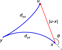
Figure 7: Illustration of the configuration of the triangle referred to in the statement of Proposition 14. The sides running from $y$ to $u$ and from $y$ to $x$ (and of intrinsic lengths $d_{yu}$ and $d_{yx}$, resp.) are intrinsic geodesics. The side running from $x$ to $u$ is a Euclidean segment.

Note also that a consequence of Proposition 12 is that intrinsic geodesics have continuously varying directions, and therefore that it makes sense to speak of the angle between a geodesic and a Euclidean segment.

Proposition 14

Suppose that $D$ is a $\operatorname{CAT}({0})$ domain, bounded in the Euclidean metric, satisfying a uniform exterior sphere condition based on radius $r>0$, and a uniform interior cone condition based on radius $\delta>0$ and angle $\alpha\in(0,\pi/2]$. For every $c_{1}>0$, there exist $c_{2},c_{3}<\infty$ such that, if $x,y\in\overline{D}$ with $\operatorname{dist}_{\mathrm{intr}}(x,y)\geq c_{1}$ and $\sqrt{|u-x|}\lor|u-x|\leq c_{2}$, then

$$\bigl{|}\operatorname{dist}_{\mathrm{intr}}(u,y)-\bigl{(}\operatorname{dist}_{\mathrm{intr}}(x,y)+|u-x|\cos\theta\bigr{)}\bigr{|}\leq c_{3}|u-x|^{3/2},$$ (13)

where $\theta$ is the angle between the geodesic from $y$ to $x$ and the Euclidean segment from $x$ to $u$ that is exterior to the direction from $y$ to $x$ (see Figure 7). Consequently, if $x$, $y\in\overline{D}$ with $x\neq y$, then

$$\operatorname{grad}_{x}\operatorname{dist}_{\mathrm{intr}}(x,y)=-\chi(x,y).$$ (14)

Moreover,

$$\operatorname{grad}\operatorname{dist}_{\mathrm{intr}}(x,y)=(-\chi(x,y),-\chi(y,x)).$$ (15)

Note that Bieske (2010) establishes a similar result for Carnot–Carathéodory spaces. In both cases, the relevant distance function satisfies an eikonal equation.

Proof of Proposition 14 In order to demonstrate (13), we establish upper and lower bounds on the difference

$$\operatorname{dist}_{\mathrm{intr}}(y,u)-\operatorname{dist}_{\mathrm{intr}}(y,x)$$ (16)

when $u$ is close to $x$. We abbreviate, setting $d_{yx}=\operatorname{dist}_{\mathrm{intr}}(y,x)$, etc.

Let $\theta^{\prime}$ be the exterior angle between the geodesic from $x$ to $y$ and the geodesic from $x$ to $u$. By the $\operatorname{CAT}({0})$ property, the Euclidean triangle with the same side lengths as a triangle in the intrinsic metric has larger interior angles and therefore smaller exterior angles. [The elementary argument for this is given in Bridson and Haefliger (1999), Chapter II.1, Proposition 1.7(4).] Thus if $\theta^{\prime\prime}$ is the exterior angle of the comparison triangle for $x,y$ and $u$ corresponding to the exterior angle $\theta^{\prime}$, then $\theta^{\prime\prime}\leq\theta^{\prime}$, and so

$$d_{yu} = \sqrt{d_{yx}^{2}+d_{xu}^{2}+2d_{yx}d_{xu}\cos\theta^{\prime\prime}}\geq\sqrt{d_{yx}^{2}+d_{xu}^{2}+2d_{yx}d_{xu}\cos\theta^{\prime}}$$

$$\geq \sqrt{d_{yx}^{2}+d_{xu}^{2}\cos^{2}\theta^{\prime}+2d_{yx}d_{xu}\cos\theta^{\prime}}=d_{yx}+d_{xu}\cos\theta^{\prime}$$

$$\geq d_{yx}+|u-x|\cos\theta^{\prime}.$$

Corollary 13 implies that $|\theta-\theta^{\prime}|\leq c_{4}d_{xu}$ for small $d_{xu}$. Hence, $|\theta-\theta^{\prime}|\leq c_{5}|u-x|$ and $|\cos\theta-\cos\theta^{\prime}|\leq c_{5}|u-x|$. We obtain for $|u-x|\leq c_{2}$, for some $c_{2}>0$,

$$\qquad d_{yu} \geq d_{yx}+|u-x|\cos\theta^{\prime}\geq d_{yx}+|u-x|\cos\theta-|u-x||\cos\theta-\cos\theta^{\prime}|$$

$$\geq d_{yx}+|u-x|\cos\theta-c_{5}|u-x|^{2}.$$

This provides a lower bound on (16) and a bound for one direction of (13).

We now establish an upper bound on (16). Fix a point $w$ on the intrinsic geodesic from $y$ to $x$. Then $d_{yx}=d_{yw}+d_{wx}$ and $d_{yu}\leq d_{yw}+d_{wu}$. We shall require $w$ to be close to $x$, but not as close as $u$, with $|w-x|=\sqrt{|u-x|}$ being assumed.

Because $w$ is close to $x$ and thus also close to $u$, we may replace the intrinsic geodesics from $w$ to $u$ and from $w$ to $x$ by Euclidean segments, without greatly altering lengths and segments. Let $\theta^{*}$ be the exterior angle at $x$ for the Euclidean triangle with sides $d_{x,w},d_{x,u}$ and $d_{u,w}$. From (11),

$$|u-w| \leq d_{wu}=\frac{d_{wu}}{|u-w|}|u-w|\leq(1+c_{6}|u-w|^{2})|u-w|,$$ (18)

$$|x-w| \leq d_{wx}=\frac{d_{wx}}{|x-w|}|x-w|\leq(1+c_{6}|x-w|^{2})|x-w|,$$ (19)

when $|u-w|$, $|x-w|<2r\sin\alpha$.

As before, by Corollary 13, $|\theta-\theta^{*}|\leq c_{7}d_{xw}$ for small $d_{xw}$. Hence, $|\theta-\theta^{*}|\leq c_{8}|w-x|$ and

$$|\cos\theta-\cos\theta^{*}|\leq c_{8}|w-x|.$$ (20)

These computations allow use to establish an upper bound for $\operatorname{dist}_{\mathrm{intr}}(y,u)-\operatorname{dist}_{\mathrm{intr}}(y,x)$. First note that

$$d_{yu} \leq d_{yw}+d_{wu}\leq d_{yw}+(1+c_{6}|u-w|^{2})|u-w|$$

$$\leq d_{yw}+|u-w|+c_{6}|u-w|^{3}$$

$$\leq d_{yw}+|u-w|+c_{6}(|u-x|+|w-x|)^{3}.$$

Now apply the cosine formula to control $|u-w|$, using (20):

$$|u-w| = \sqrt{|w-x|^{2}+|u-x|^{2}+2|w-x||u-x|\cos\theta^{*}}$$

$$= \bigl{(}(|w-x|+|u-x|\cos\theta)^{2}+|u-x|^{2}\sin^{2}\theta$$

$$\hskip 40.0pt{}+2|w-x||u-x|(\cos\theta^{*}-\cos\theta)\bigr{)}^{1/2}$$

$$\leq |w-x|+|u-x|\cos\theta$$

$${}+\frac{1}{2}\frac{|u-x|^{2}\sin^{2}\theta}{|w-x|+|u-x|\cos\theta}+\frac{|w-x||u-x|(\cos\theta^{*}-\cos\theta)}{|w-x|+|u-x|\cos\theta}$$

$$\leq |w-x|+|u-x|\cos\theta+\frac{1}{2}\frac{|u-x|^{2}\sin^{2}\theta}{|w-x|-|u-x|}$$

$${}+\frac{|w-x||u-x|}{|w-x|-|u-x|}c_{8}|w-x|.$$

If we take $|w-x|=\sqrt{|u-x|}$, with $|u-x|<c_{9}$ for a suitably small $c_{9}>0$, then

$$|u-w|\leq|w-x|+|u-x|\cos\theta+c_{10}|u-x|^{3/2}.$$

Combining these bounds implies

$$d_{yu} \leq d_{yw}+|u-w|+c_{6}(|u-x|+|w-x|)^{3}$$

$$\leq d_{yw}+|w-x|+|u-x|\cos\theta+c_{10}|u-x|^{3/2}+c_{6}(|u-x|+|w-x|)^{3}$$

$$\leq d_{yw}+d_{w,x}+|u-x|\cos\theta+c_{11}|u-x|^{3/2}$$

$$= d_{yx}+|u-x|\cos\theta+c_{11}|u-x|^{3/2},$$

which provides an upper bound on (16). It follows from the above inequality and (2.1) that

$$\bigl{|}d_{yu}-(d_{yx}+|u-x|\cos\theta)\bigr{|}\leq c_{3}|u-x|^{3/2},$$

which yields the bound in (13). The formula in (14), for the gradient of the intrinsic distance $\operatorname{dist}_{\mathrm{intr}}(x,y)$ with respect to $x$, follows immediately.

We still need to demonstrate the formula in (15). Let $c_{1},c_{2}$ and $c_{3}$ be as in the statement of (13). Fix $x,y\in\overline{D}$ and suppose that $\operatorname{dist}_{\mathrm{intr}}{(x,y)}\geq 2c_{1}$. Suppose that $u,v\in\overline{D}$, $\sqrt{|u-x|}\lor|u-x|\leq c_{2}\land c_{1}/4$ and $\sqrt{|v-y|}\lor|v-y|\leq c_{2}\land c_{1}/4$. Let $\theta_{x}$ be the exterior angle between the geodesic from $x$ to $y$ and the Euclidean segment from $x$ to $u$. Similarly, let $\theta_{y}$ be the exterior angle between the geodesic from $y$ to $x$ and the Euclidean segment from $y$ to $v$. Also, let $\theta^{\prime}$ be the exterior angle between the geodesic from $y$ to $u$ and the Euclidean segment from $y$ to $v$. Then by the above reasoning

$$\bigl{|}\operatorname{dist}_{\mathrm{intr}}(u,y)-\bigl{(}\operatorname{dist}_{\mathrm{intr}}(x,y)+|u-x|\cos\theta_{x}\bigr{)}\bigr{|}\leq c_{3}|u-x|^{3/2}$$ (21)

and

$$\bigl{|}\operatorname{dist}_{\mathrm{intr}}(v,u)-\bigl{(}\operatorname{dist}_{\mathrm{intr}}(y,u)+|v-y|\cos\theta^{\prime}\bigr{)}\bigr{|}\leq c_{3}|v-y|^{3/2}.$$ (22)

Recall that the Euclidean triangle with the same side lengths as a triangle in intrinsic metric has larger interior angles. Using a triangle inequality for angles, $|\theta_{y}-\theta^{\prime}|$ is less than the angle at the vertex corresponding to $y$ in the Euclidean triangle with sides $d_{xy},d_{xu}$ and $d_{yu}$. It follows that $|\theta_{y}-\theta^{\prime}|\leq c_{12}d_{xu}/d_{xy}\leq c_{13}|u-x|$ and therefore $|\cos\theta_{y}-\cos\theta^{\prime}|\leq c_{13}|u-x|$. This and (22) yield

$$\bigl{|}\operatorname{dist}_{\mathrm{intr}}(v,u)-\bigl{(}\operatorname{dist}_{\mathrm{intr}}(y,u)+|v-y|\cos\theta_{y}\bigr{)}\bigr{|}$$

(23)

$$\qquad\leq c_{3}|v-y|^{3/2}+c_{13}|u-x||v-y|.$$

The triangle inequality applied to the left-hand sides of (21) and (2.1) implies that

$$\bigl{|}\operatorname{dist}_{\mathrm{intr}}(v,u)-\bigl{(}\operatorname{dist}_{\mathrm{intr}}(x,y)+|v-y|\cos\theta_{y}+|u-x|\cos\theta_{x}\bigr{)}\bigr{|}$$

$$\quad\leq c_{3}|u-x|^{3/2}+c_{3}|v-y|^{3/2}+c_{13}|u-x||v-y|.$$

Consequently, $\operatorname{grad}\operatorname{dist}_{\mathrm{intr}}(x,y)$ exists when $\operatorname{dist}_{\mathrm{intr}}(x,y)$ is viewed as a function of $(x,y)\in(\overline{D}\times\overline{D})\setminus\{(u,u)\dvtx u\in\overline{D}\}$ and is given by

$$\operatorname{grad}\operatorname{dist}_{\mathrm{intr}}(x,y)=(-\chi(x,y),-\chi(y,x)).$$

In Proposition 15, we consider solutions of the differential equation $\mathrm{d}x=\chi(x,y)\,\mathrm{d}t$ for pursuit and evasion. Proposition 12 established partial regularity for $\chi(x,y)$, which does not automatically guarantee well-posedness of solutions (as defined below). However, the $\operatorname{CAT}({0})$ property, together with boundary regularity, will imply well-posedness, even for some discontinuous driving paths $y$.

Suppose that $y(t)$, $t\in[0,T_{1}]$, is cadlag, of bounded variation on finite intervals, and takes values in $\overline{D}$. We will say that $x(t)$, $t\in[0,T_{1}]$, is a weak solution to $\mathrm{d}x=\chi(x,y)\,\mathrm{d}t$ if $x(t)=x(0)+\int_{0}^{t}\chi(x(s),y(s))\,\mathrm{d}s$ for all $t\in[0,T_{1}]$.

Proposition 15

Let $D$ be a $\operatorname{CAT}({0})$ domain satisfying uniform exterior sphere and interior cone conditions. For distinct $x,y\in\overline{D}$, let $\chi(x,y)$ be the unit tangent vector at $x$ of the geodesic from $x$ to $y$. We consider the differential equation

$$\mathrm{d}x=\chi(x,y)\,\mathrm{d}t$$ (24)

defined in the weak sense for absolutely continuous paths $\{x(t)\dvtx t\geq 0\}$ in $\overline{D}$, driven by paths $\{y(t)\dvtx t\geq 0\}$, up until the first time that $x$ and $y$ are equal. The problem is well-posed, in the sense that solutions $x$ exist, are uniquely determined by initial values $x(0)$, and depend continuously on the initial value $x(0)$ and the driving process $\{y(t)\dvtx t\geq 0\}$ (using the uniform distance metric in both cases).

The argument is based on the simpler case when the path $y$ is constant in time, which we for the moment assume. In this case, existence follows directly from the existence of intrinsic geodesics in $\operatorname{CAT}({0})$ domains. To show uniqueness, note that, for two solutions $x$ and $\widetilde{x}$ of (24), since $x$ and $\widetilde{x}$ are absolutely continuous and satisfy the differential equation weakly, for almost all $s$, the time-derivatives of $x(s)$ and $\widetilde{x}(s)$ must exist and be given by $\chi(x(s),y)$ and $\chi(\widetilde{x}(s),y)$. Exploiting the differentiability of the intrinsic distance given by Proposition 14, for $x(s)\neq y$ and $\widetilde{x}(s)\neq y$, one has

$$\qquad\biggl{[}\frac{\mathrm{d}}{\mathrm{d}t}\operatorname{dist}_{\mathrm{intr}}\bigl{(}x(s+t),\widetilde{x}(s+t)\bigr{)}\biggr{]}_{t=0}=\biggl{[}\frac{\mathrm{d}}{\mathrm{d}t}\operatorname{dist}_{\mathrm{intr}}\bigl{(}\Gamma^{(s)}(t),\widetilde{\Gamma}^{(s)}(t)\bigr{)}\biggr{]}_{t=0},$$ (25)

where $\Gamma^{(s)}$, $\widetilde{\Gamma}^{(s)}$ are unit-speed geodesics running from $x(s)$, $\widetilde{x}(s)$ to $y$. We will show that

$$\biggl{[}\frac{\mathrm{d}}{\mathrm{d}t}\operatorname{dist}_{\mathrm{intr}}\bigl{(}\Gamma^{(s)}(t),\widetilde{\Gamma}^{(s)}(t)\bigr{)}\biggr{]}_{t=0}\leq 0.$$ (26)

Consider a Euclidean triangle $abc$ with side lengths satisfying $|ab|=\break\operatorname{dist}_{\mathrm{intr}}({\Gamma}^{(s)}(0),y)$, $|cb|=\operatorname{dist}_{\mathrm{intr}}(\widetilde{\Gamma}^{(s)}(0),y)$ and $|bc|=\operatorname{dist}_{\mathrm{intr}}({\Gamma}^{(s)}(0),\widetilde{\Gamma}^{(s)}(0))$. Let $z(t)\in ab$ be a point such that $|z(t)-a|=t$, and let $\widetilde{z}(t)\in bc$ be a point such that $|\widetilde{z}(t)-c|=t$. Then Definition 4 implies that

$$\operatorname{dist}_{\mathrm{intr}}\bigl{(}{\Gamma}^{(s)}(t),\widetilde{\Gamma}^{(s)}(t)\bigr{)}\leq|z(t)-\widetilde{z}(t)|\leq|z(0)-\widetilde{z}(0)|=\operatorname{dist}_{\mathrm{intr}}\bigl{(}{\Gamma}^{(s)}(0),\widetilde{\Gamma}^{(s)}(0)\bigr{)}.$$

This implies (26). It follows that the derivative on the left-hand side of (25) is nonpositive; therefore $x=\widetilde{x}$ if $x(0)=\widetilde{x}(0)$, and so uniqueness holds.

By considering the behaviour over disjoint time intervals, existence and uniqueness follow for the case when $y$ is piecewise-constant, in which case the solution curve $x$ is piecewise-geodesic.

We will establish continuous dependence on the initial position $x(0)$ and the driving process $y$, when $y$ is piecewise constant. Suppose that $y$, $\widetilde{y}$ are two piecewise-constant paths in $\overline{D}$, and $x$, $\widetilde{x}$ solve

$$\mathrm{d}x=\chi(x,y)\,\mathrm{d}t,\qquad\mathrm{d}\widetilde{x}=\chi(\widetilde{x},\widetilde{y})\,\mathrm{d}t$$

for prescribed initial positions $x(0)\neq y(0)$ and $\widetilde{x}(0)\neq\widetilde{y}(0)$. The solutions $x$, $\widetilde{x}$ satisfy the differential equations weakly, and therefore, for almost all $s$, the time-derivatives of $x(s)$ and $\widetilde{x}(s)$ must exist and are given by $\chi(x(s),y(s))$ and $\chi(\widetilde{x}(s),\widetilde{y}(s))$. Arguing as before, for $x(s)\neq y(s)$ and $\widetilde{x}(s)\neq\widetilde{y}(s)$, we may construct a $\operatorname{CAT}({0})$ comparison for the two triangles defined by (a) vertices $x(s)$, $\widetilde{x}(s)$, $y(s)$ and (b) vertices $\widetilde{x}(s)$, $\widetilde{y}(s)$, $y(s)$ (see Figure 8). Using this comparison, and continuing until either $x(t)=y(t)$ or $\widetilde{x}(t)=\widetilde{y}(t)$, the function $\operatorname{dist}_{\mathrm{intr}}(x,\widetilde{x})$ is dominated by its Euclidean counterpart for a two-dimensional quadrilateral which is based on a pair of opposing sides of lengths $\operatorname{dist}_{\mathrm{intr}}(x(s),\widetilde{x}(s))$ and $\operatorname{dist}_{\mathrm{intr}}(y(s),\widetilde{y}(s))$.

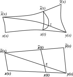
Figure 8: Illustration of the $\operatorname{CAT}({0})$ comparison argument applied to the triangles defined by vertices (a) $x(s)$, $\widetilde{x}(s)$, $y(s)$ and (b) $\widetilde{x}(s)$, $\widetilde{y}(s)$, $y(s)$. The corresponding Euclidean triangles have vertices marked with boldface symbols.

In detail, and using boldface symbols to indicate corresponding Euclidean comparison points, we may argue as follows (see Figure 8). Because side-lengths of comparison triangles agree,

$$\operatorname{dist}_{\mathrm{intr}}(x(s),y(s)) = |\mathbf{x}(\mathbf{s})-\mathbf{y}(\mathbf{s})|,$$

$$\operatorname{dist}_{\mathrm{intr}}(\widetilde{x}(s),y(s)) = |\widetilde{\mathbf{x}}(\mathbf{s})-\mathbf{y}(\mathbf{s})|,$$

$$\operatorname{dist}_{\mathrm{intr}}(x(s),\widetilde{x}(s)) = |\mathbf{x}(\mathbf{s})-\widetilde{\mathbf{x}}(\mathbf{s})|,$$

$$\operatorname{dist}_{\mathrm{intr}}(\widetilde{x}(s),\widetilde{y}(s)) = |\widetilde{\mathbf{x}}(\mathbf{s})-\widetilde{\mathbf{y}}(\mathbf{s})|,$$

$$\operatorname{dist}_{\mathrm{intr}}(y(s),\widetilde{y}(s)) = |\mathbf{y}(\mathbf{s})-\widetilde{\mathbf{y}}(\mathbf{s})|.$$

Locating $x(t)$ according to distance from $x(s)$ along the intrinsic geodesic from $x(s)$ to $y(s)$, and $\widetilde{x}(t)$ according to distance from $\widetilde{x}(s)$ along the intrinsic geodesic from $\widetilde{x}(s)$ to $\widetilde{y}(s)$ (and locating comparison Euclidean points in the corresponding way), we find

$$\operatorname{dist}_{\mathrm{intr}}(x(s),x(t)) = |\mathbf{x}(\mathbf{s})-\mathbf{x}(\mathbf{t})|,$$

$$\operatorname{dist}_{\mathrm{intr}}(\widetilde{x}(s),\widetilde{x}(t)) = |\widetilde{\mathbf{x}}(\mathbf{s})-\widetilde{\mathbf{x}}(\mathbf{t})|.$$

Now locate the Euclidean point $\mathbf{z}$ at the intersection of the Euclidean line segments $\overline{\widetilde{\mathbf{x}}(\mathbf{s}),\mathbf{y}(\mathbf{s})}$ and $\overline{\mathbf{x}(\mathbf{t}),\widetilde{\mathbf{x}}(\mathbf{t})}$, and locate $z$ on the intrinsic geodesic from $\widetilde{x}(s)$ to $y(s)$ so that

$$\operatorname{dist}_{\mathrm{intr}}(\widetilde{x}(s),z)=|\widetilde{\mathbf{x}}(\mathbf{s})-\mathbf{z}|.$$

Using comparison arguments and the nature of the Euclidean parallelogram $\mathbf{x}(\mathbf{s})\widetilde{\mathbf{x}}(\mathbf{s})\widetilde{\mathbf{y}}(\mathbf{s})\mathbf{y}(\mathbf{s})$, we then see that

$$\operatorname{dist}_{\mathrm{intr}}(x(t),\widetilde{x}(t)) \leq \operatorname{dist}_{\mathrm{intr}}(x(t),z)+\operatorname{dist}_{\mathrm{intr}}(z,\widetilde{x}(t))$$

$$\leq |\mathbf{x}(\mathbf{t})-\mathbf{z}|+|\mathbf{z}-\widetilde{\mathbf{x}}(\mathbf{t})|=|\mathbf{x}(\mathbf{t})-\widetilde{\mathbf{x}}(\mathbf{t})|$$

$$\leq \max\{|\mathbf{x}(\mathbf{s})-\widetilde{\mathbf{x}}(\mathbf{s})|,|\mathbf{y}(\mathbf{s})-\widetilde{\mathbf{y}}(\mathbf{s})|\}$$

$$= \max\{\operatorname{dist}_{\mathrm{intr}}(x(s),\widetilde{x}(s)),\operatorname{dist}_{\mathrm{intr}}(y(s),\widetilde{y}(s))\}.$$

This comparison can also be justified by use of Reshetnyak majorization, however we have chosen to present an explicit elementary proof.

We now consider general $y$ in (24). There exist piecewise-constant functions $y_{n}$ converging to $y$ uniformly on compact intervals; let $x_{n}$ be the corresponding solutions to (24), with $x_{n}(0)=x(0)\in\overline{D}$. If $|y_{n}(t)-y_{m}(t)|\leq c_{1}$ for $t\in[0,T]$, then $|x_{n}(t)-x_{m}(t)|\leq c_{1}$ by the argument given above. Since the sequence $y_{n}$ is Cauchy in the uniform norm on $[0,T]$, so is the sequence $x_{n}$, which therefore converges to a function $x$.

Recall that we are assuming $x(0)\neq y(0)$. Choose fixed $\varepsilon_{1},\varepsilon_{2}>0$ and let $T=\inf\{t>0\dvtx|x(t-)-y(t-)|\leq 2\varepsilon_{1}\}$. By part (3) of Proposition 12, there exists $\delta_{1}>0$ such that, if $|u_{1}-u_{2}|\geq\varepsilon_{1}$, $|v_{1}-v_{2}|\geq\varepsilon_{1}$, $|u_{1}-v_{1}|\leq\delta_{1}$ and $|u_{2}-v_{2}|\leq\delta_{1}$, then $|\chi(u_{1},u_{2})-\chi(v_{1},v_{2})|\leq\varepsilon_{2}/T$. Suppose that $n$ is large enough so that $|y_{n}(t)-y(t)|\leq\delta_{1}\land\varepsilon_{1}$ for $t\in[0,T]$. Then $|x_{n}(t)-x(t)|\leq\delta_{1}\land\varepsilon_{1}$ for $t\in[0,T]$ and $|\chi(x(t),y(t))-\chi(x_{n}(t),y_{n}(t))|\leq\varepsilon_{2}/T$. We obtain, for $t\leq T$,

$$\biggl{|}x(t)-x(0)-\int_{0}^{t}\chi(x(s),y(s))\,\mathrm{d}s\biggr{|}$$

$$\qquad\leq|x(t)-x_{n}(t)|+\biggl{|}x_{n}(t)-x(0)-\int_{0}^{t}\chi(x_{n}(s),y_{n}(s))\,\mathrm{d}s\biggr{|}$$

$$\qquad\quad{}+\biggl{|}\int_{0}^{t}\chi(x_{n}(s),y_{n}(s))\,\mathrm{d}s-\int_{0}^{t}\chi(x(s),y(s))\,\mathrm{d}s\biggr{|}$$

$$\qquad\leq\delta_{1}+0+\int_{0}^{t}|\chi(x_{n}(s),y_{n}(s))-\chi(x(s),y(s))|\,\mathrm{d}s$$

$$\qquad\leq\delta_{1}+\varepsilon_{2}.$$

Since $\varepsilon_{1},\varepsilon_{2}$ and $\delta_{1}$ can be chosen arbitrarily small, we see that $x(t)=x(0)+\int_{0}^{t}\chi(x(s),y(s))\,\mathrm{d}s$ for all $t<\inf\{t>0\dvtx|x(t-)-y(t-)|=0\}$. Hence, $x$ is a solution to (24).

Uniqueness of the solution of (24), for given $x(0)$ and general $y$, follows by reasoning as in (25) and (26). The continuous dependence of solutions on $x(0)$ and $y$, for general $y$, follows from the above estimates by approximating $y$ by piecewise constant driving processes.

3 $\operatorname{CAT}({0})$ and pursuit–evasion.

We consider the Lion and Man problem in a bounded $\operatorname{CAT}({0})$ domain $D$ satisfying the uniform exterior sphere and interior cone conditions. Alexander, Bishop and Ghrist (2006) showed that $\varepsilon/2$-capture, for given $\varepsilon>0$, must occur for the discrete-time variant of this problem. As we will see in Section 4, the Lion and Man trajectories $x$ and $y$ will be weak limits of couplings of reflected Brownian motions, with drift and small noise, that arise from our capture problem.

We therefore modify the Alexander, Bishop and Ghrist (2006) argument to apply to continuous time; the modified argument also supplies an explicit upper bound on the capture time. We will only need to consider trajectories $x$ and $y$ that are Lipschitz with constant $1$. Note that Lipschitz trajectories are absolutely continuous, so that the directions $\mathrm{d}x/\mathrm{d}t$ and $\mathrm{d}y/\mathrm{d}t$ are defined for almost all times $t$.

One can express the trajectories of Lion $x$ and Man $y$ as functions of time $t$ in the following differential form:

$$\mathrm{d}x = \chi(x,y)\,\mathrm{d}t-\nu_{x}\,\mathrm{d}L^{x},$$

$$\mathrm{d}y = H\,\mathrm{d}t-\nu_{y}\,\mathrm{d}L^{y}.$$

Here, $H$ is assumed to be a pre-assigned, time-varying unit length vector generating the motion of the Man, $\chi(x,y)$ generates the motion of the Lion and is defined as in Proposition 12, for $x\neq y$, as the unit tangent at $x$ for the corresponding intrinsic geodesic, while $\nu_{x}\in\mathcal{N}_{x,r}$ and $\nu_{y}\in\mathcal{N}_{y,r}$ (for $r>0$ satisfying the exterior sphere condition of $D$ as given in Definition 6) determine the reflection off of the boundary $\partial D$. The vector $H$ is assumed to be measurable in $t$; on account of Proposition 12, $\chi$ is continuous on $x\neq y$. The terms $\nu_{x}\,\mathrm{d}L^{x}$, respectively, $\nu_{y}\,\mathrm{d}L^{y}$, are differentials arising from Skorokhod transformations and are differentials of functions of bounded variation that increase only when $x$, respectively, $y$, belong to $\partial D$, and are then directed along an outward-pointing unit normal so as to cancel exactly with the outward-pointing component of the drifts $\chi\,\mathrm{d}t$, respectively, $H\,\mathrm{d}t$.

We note that Skorokhod transformations are uniquely defined for a domain satisfying uniform exterior sphere and interior cone conditions [Saisho (1987)] [also compare earlier results of Lions and Sznitman (1984)], and they then depend continuously on the driving processes (using the uniform path metric). In fact, by the definition of $\chi$, $\nu_{x}\,\mathrm{d}L^{x}$ vanishes identically, while $\nu_{y}\,\mathrm{d}L^{y}$ vanishes identically if $\langle H,\nu\rangle<0$ whenever $y\in\partial D$. In particular, Proposition 15 applies and guarantees the existence of $x$ and its approximation by piecewise-geodesic paths for $y$ determined by $H$. [We include both the Skorokhod transformation differentials in (3) as they will both appear in the stochastic version in Section 4.]

We base our argument on Alexander, Bishop and Ghrist [(2006), Theorem 12]. The proof analyzes the greedy pursuit strategy arising from the definition of the vector field $\chi$, with the Lion always directing its motion along the intrinsic geodesic from Lion to Man. The $\operatorname{CAT}({0})$ property forces the distance between Lion and Man to be nonincreasing, and the Man must run directly away from the Lion in order to prolong successful evasion. Since the domain is bounded, this will, however, not be achievable indefinitely.

In order to demonstrate the main result in this section, Proposition 17, we will employ the following lemma.

Lemma 16

Under the greedy pursuit strategy described above, in a$\operatorname{CAT}({0})$ domain satisfying uniform exterior sphere and interior cone conditions, and at a time $t$ at which Lion and Man locations $x(t)$ and $y(t)$ are differentiable in $t$,

$$\frac{\mathrm{d}}{\mathrm{d}t}\operatorname{dist}_{\mathrm{intr}}(x(t),y(t))=-\bigl{(}1-|y^{\prime}(t)|\cos\alpha(t)\bigr{)},$$

where $\alpha(t)$ is the angle between the Man’s velocity $y^{\prime}(t)$ and the geodesic running from Lion to Man.

This follows immediately from the generalization of Gauss’ lemma to such domains, as was established in Proposition 14.

Alternatively, Lemma 16 follows directly from the first variation formula in $\operatorname{CAT}({0})$ spaces [Bridson and Haefliger (1999), page 185, Burago, Burago and Ivanov (2001), Exercise 4.5.10].

Proposition 17

Suppose that $D$ is a bounded $\operatorname{CAT}(0)$ domain that satisfies a uniform exterior sphere condition based on a radius $r>0$ and a uniform interior cone condition based on a radius $\delta>0$ and angle $\alpha\in(0,\pi/2]$. Under the greedy pursuit strategy described above, there is a positive constant $t_{c}$ depending only on the diameter of $D$ and $\varepsilon>0$ [and not on $H$ in (3)] such that the Lion will come within distance $\varepsilon/2$ of the Man before time $t_{c}$, regardless of their starting positions within $D$.

We use $\varepsilon/2$ here rather than $\varepsilon$, since a further distance $\varepsilon/2$ will be required by the stochastic part of the argument.

Proof of Proposition 17 This proof follows Alexander, Bishop and Ghrist (2006), but is modified (a) to account for the continuous time context and (b) because we need to derive a specific upper bound $t_{c}$ on the time of $\varepsilon/2$-capture. Below, we abbreviate by setting $\mathcal{L}(t)=\operatorname{dist}_{\mathrm{intr}}(x(t),y(t))$.

Let $\alpha$ be the angle defined in Lemma 16. Note that this is defined for almost all times $t$, since the paths $x(t)$, $y(t)$ are Lipschitz and are therefore differentiable for almost all $t$. Evidently, the Lion will have come within $\varepsilon/2$ of the Man by time $t$ unless

$$\int^{t}_{0}(1-\cos\alpha)\,\mathrm{d}s<\mathcal{L}(0)-\varepsilon/2\leq\operatorname{diam}_{\mathrm{intr}}(D)-\varepsilon/2.$$ (28)

Now consider the total curvature of the Lion’s path. By Proposition 15, the Lion’s path is uniformly approximated by pursuit paths driven by discretized approximations to the Man’s path. If $x^{(n)}$ is the Lion’s path driven by a discretized Man’s path $y^{(n)}$, then the Lion’s path is piecewise-geodesic, with total absolute curvature given by the sum of the exterior angles formed at the points that connect the geodesics that occur when $x^{(n)}$ changes direction. $\operatorname{CAT}({0})$ comparison bounds then show the total curvature of $x^{(n)}$ is bounded above by

$$\sum\frac{\sin\alpha^{(n)}}{\operatorname{dist}_{\mathrm{intr}}(x^{(n)},y^{(n)})}\Delta y^{(n)},$$ (29)

where summation is over the jumps of the discretized path $y^{(n)}$, and $\alpha^{(n)}$ is the exterior angle that the jump $\Delta y^{(n)}$ contributes to the geodesic running from $x^{(n)}$ to $y^{(n)}$.

The total curvature of a path is a lower-semicontinuous function of the path (using the uniform topology) for $\operatorname{CAT}({0})$ spaces. [This is a special case of a $\operatorname{CAT}({\kappa})$ result of Karuwannapatana and Maneesawarng (2007), referred to in Alexander, Bishop and Ghrist (2010), Theorem 18.] For the sake of completeness, we indicate the short proof for the $\operatorname{CAT}({0})$ case. Consider a curve $q$ of finite length in a $\operatorname{CAT}({0})$ space. Its total curvature $\operatorname{TC}(q)$ is the supremum of sums of exterior angles of piecewise-geodesic curves interpolating $q$; a $\operatorname{CAT}({0})$ comparison argument shows that these sums of exterior angles increase as the interpolating mesh is refined. Let $q^{n}$ be a sequence of curves converging uniformly to $q$. Furthermore, let $q^{n,m}$ be the piecewise-geodesic curve interpolating $q^{n}$ at the points $k2^{-m}$ for $k=0,1,\ldots.$ Then, by definition of total curvature,

$$\operatorname{TC}(q^{n,m})\nearrow\operatorname{TC}(q^{n})\qquad\mbox{as }m\to\infty.$$

Bridson and Haefliger [(1999), Chapter II.3 Proposition 3.3] observe that the $\operatorname{CAT}({0})$ property implies that interior angles are continuous functions of their end vertices and upper-semicontinuous functions of their centre vertices. This upper-semicontinuity translates into lower-semicontinuity for exterior angles, and hence

$$\limsup_{n\to\infty}\operatorname{TC}(q^{n,m})\geq\operatorname{TC}(q^{\infty,m}),$$

where $q^{\infty,m}$ is the uniform limit of $q^{n,m}$ as $n\to\infty$ [here we use the $\operatorname{CAT}({0})$ property again] and is a piecewise-geodesic interpolation of $q$ at the points $k2^{-m}$ for $k=0,1,\ldots.$ Since $\operatorname{TC}(q)=\lim\operatorname{TC}(q^{\infty,m})$, lower-semicontinuity now follows from

$$\limsup_{n\to\infty}\operatorname{TC}(q^{n})\geq\limsup_{n\to\infty}\operatorname{TC}(q^{n,m})\geq\operatorname{TC}(q^{\infty,m})\to\operatorname{TC}(q)\qquad\mbox{as }m\to\infty.$$

Consequently, the upper bound (29) provides an upper bound on the total absolute curvature of the Lion’s path in the limit. Bearing in mind the $\operatorname{Lipschitz}(1)$ property of $y$, the total absolute curvature $\tau(t)$ incurred by $x$ between times $0$ and $t$ therefore satisfies

$$\tau(t)\leq\int_{0}^{t}\frac{|\sin\alpha(s)|}{\mathcal{L}(s)}\,\mathrm{d}s.$$ (30)

Assume that $\mathcal{L}(s)\geq\varepsilon/2$ for $s\leq t$. By the Cauchy–Schwarz inequality and (28),

$$\tau(t) \leq \frac{2}{\varepsilon}\int_{0}^{t}|\sin\alpha|\,\mathrm{d}s\leq\frac{2}{\varepsilon}\sqrt{t\int_{0}^{t}\sin^{2}\alpha\,\mathrm{d}s}$$

$$\leq \frac{2\sqrt{2}}{\varepsilon}\sqrt{t\int_{0}^{t}(1-\cos\alpha)\,\mathrm{d}s}\leq\frac{2\sqrt{2}}{\varepsilon}\sqrt{\operatorname{diam}_{\mathrm{intr}}(D)-\varepsilon/2}\cdot\sqrt{t}.$$

Next, we follow Alexander, Bishop and Ghrist (2006) in applying Reshetnyak majorization [Rešetnjak (1968); see also the telegraphic description in Berestovskij and Nikolaev (1993), Section 7.4] to generate a lower bound on the total absolute curvature of $\{x(s)\dvtx 0\leq s\leq t\}$. We provide details for the sake of completeness.

We argue as follows. Reshetnyak majorization asserts that for every closed curve $\zeta$ in $\overline{D}$ [more generally, in any $\operatorname{CAT}({0})$ space], one can construct a convex planar set $C$, bounded by a closed unit-speed curve $\overline{\zeta}$, and a distance-nonincreasing continuous map $\phi\dvtx C\to\overline{D}$ such that $\phi\circ\overline{\zeta}=\zeta$; moreover, $\phi$ preserves the arc-length distances along $\phi\circ\overline{\zeta}$ and $\zeta$. Consequently, $\phi$ restricted to $\partial C$ will not increase angles and the pre-images under $\phi$ of geodesic segments in $\zeta$ must themselves be Euclidean geodesics (i.e., line segments).

By our assumptions about $t$, the total absolute curvature of $\{x(s)\dvtx 0\leq s\leq t\}$ is finite [see (3)]. Fix an arbitrarily small $\delta_{1}\in(0,\pi/2)$. It follows from the definitions of length and curvature of a path that, for each $n$, we can approximate the unit-speed curve $\{x(s)\dvtx 0\leq s\leq t\}$ by a piecewise-geodesic curve $\{z(s)\dvtx 0\leq s\leq t^{\prime}\}$ with the following properties:

• The curve $z$ is parametrized using arc-length.

• Note that $x$ and $y$ are continuous, so is $\chi(x,y)$, by Proposition 12(3). Hence, we can choose $0=t_{0}<t_{1}<\cdots<t_{n}=t$ such that the total absolute curvature of $\{x(s)\dvtx t_{i-1}\leq s\leq t_{i}\}$ is equal to $\pi/2-\delta_{1}$ for all $i$, with the possible exception of $i=n$.

• For every $i$, there exist $t_{i}=t_{i}^{0}<t_{i}^{1}<\cdots<t_{i}^{m_{i}}=t_{i+1}$ and $s_{i}=s^{0}_{i}<s^{1}_{i}<\cdots<s_{i}^{m_{i}}=s_{i+1}$ such that $z(s_{i}^{j})=x(t_{i}^{j})$ and $z$ is geodesic on $[s_{i}^{j},s_{i}^{j+1}]$, for all $i$ and $j$. (Notice that the curve $z$ is inscribed in the curve $x$.)

• The total absolute curvature of $\{z(s)\dvtx s_{i-1}\leq s\leq s_{i}\}$ is less than $\pi/2$. In other words, the sum (over $j$) of exterior angles between $\{z(s)\dvtx s_{i}^{j-1}\leq s\leq s_{i}^{j}\}$ and $\{z(s)\dvtx s_{i}^{j}\leq s\leq s_{i}^{j+1}\}$ at $s_{i}^{j}$ is less than $\pi/2$. [This is a consequence of $z$ being inscribed in $x$ and the $\operatorname{CAT}({0})$ property.]

• The difference between the lengths of $\{z(s)\dvtx 0\leq s\leq t^{\prime}\}$ and $\{x(s)\dvtx 0\leq s\leq t\}$ is less than $\delta_{1}$.

Then we have

$$\mbox{total absolute curvature}\bigl{(}\{x(s)\dvtx 0\leq s\leq t\}\bigr{)}\geq\biggl{(}\frac{\pi}{2}-\delta_{1}\biggr{)}(n-1).$$ (32)

We apply Reshetnyak majorization to the closed curve formed by $\{z(s)\dvtx\break s_{i-1}\leq s\leq s_{i}\}$ and its chord [the geodesic running from $z(t_{i})$ back to $z(t_{i-1})$]. Reshetnyak majorization guarantees that the total absolute curvature of $\{z(s)\dvtx s_{i-1}\leq s\leq s_{i}\}$ dominates the curvature of its pre-image in the boundary of a convex planar set $C_{i}$. Moreover, the perimeter of its pre-image in the boundary $C_{i}$ has length $\operatorname{len}(\{z(s)\dvtx s_{i-1}\leq s\leq s_{i}\})$, while the remainder of the boundary of $C_{i}$ must be a line segment of length $\operatorname{dist}_{\mathrm{intr}}(z(s_{i}),z(s_{i-1}))$.

The two-dimensional pre-image of $\{z(s)\dvtx s_{i-1}\leq s\leq s_{i}\}$ therefore has total curvature bound of $\frac{\pi}{2}$. By two-dimensional Euclidean geometry, we can maximize the ratio of the length of the pre-image of $\{z(s)\dvtx s_{i-1}\leq s\leq s_{i}\}$ to the length $\operatorname{dist}_{\mathrm{intr}}(z(s_{i}),z(s_{i-1}))$ of its chord by considering the case of an isoceles right-angled triangle, in which case the ratio is $\sqrt{2}$. Accordingly, we obtain the upper bound

$$\operatorname{len}\bigl{(}\{z(s)\dvtx s_{i-1}\leq s\leq s_{i}\}\bigr{)}\leq\sqrt{2}\operatorname{dist}_{\mathrm{intr}}(z(s_{i}),z(s_{i-1}))\leq\sqrt{2}\operatorname{diam}_{\mathrm{intr}}(D).$$

It follows that a portion of the piecewise geodesic curve $z$ which turns no more than $\frac{\pi}{2}$ cannot have length exceeding $\sqrt{2}$ times the intrinsic diameter of the region. (Note this is related to the Euclidean diameter by Lemma 10.) This implies that we can control the total length of $z$ and thus the total length of $x$, with

$$t-\delta_{1} = \operatorname{len}\bigl{(}\{x(s)\dvtx 0\leq s\leq t\}\bigr{)}-\delta_{1}$$

$$\leq \operatorname{len}\bigl{(}\{z(s)\dvtx 0\leq s\leq t\}\bigr{)}\leq\sqrt{2}\operatorname{diam}_{\mathrm{intr}}(D)\times n.$$

Combining inequalities (32) and (3), we deduce that

$$\mbox{total absolute curvature}\bigl{(}\{x(s)\dvtx 0\leq s\leq t\}\bigr{)}$$

$$\qquad\geq\biggl{(}\frac{\pi}{2}-\delta_{1}\biggr{)}(n-1)$$ (34)

$$\qquad\geq\biggl{(}\frac{\pi}{2}-\delta_{1}\biggr{)}\biggl{(}\frac{t-\delta_{1}}{\sqrt{2}\operatorname{diam}_{\mathrm{intr}}(D)}-1\biggr{)}.$$

Recall that $\tau(t)=\mbox{total absolute curvature}(\{x(s)\dvtx 0\leq s\leq t\})$ and $\operatorname{len}(\{x(s)\dvtx\break 0\leq s\leq t\})=t$. Letting $\delta_{1}\to 0$ in (3), it follows that

$$\frac{\tau(t)}{t}\geq\frac{\pi}{2}\biggl{(}\frac{1}{\sqrt{2}\operatorname{diam}_{\mathrm{intr}}(D)}-\frac{1}{t}\biggr{)}.$$

In combination with (3), this yields

$$\frac{\pi}{2}\biggl{(}\frac{1}{\sqrt{2}\operatorname{diam}_{\mathrm{intr}}(D)}-\frac{1}{t}\biggr{)}\leq\frac{2\sqrt{2}}{\varepsilon}\sqrt{\operatorname{diam}_{\mathrm{intr}}(D)-\varepsilon/2}\cdot\frac{1}{\sqrt{t}}$$

and hence the quadratic inequality for $q=\sqrt{t}$,

$$\biggl{(}\frac{\pi}{2}\frac{1}{\sqrt{2}\operatorname{diam}_{\mathrm{intr}}(D)}\biggr{)}q^{2}-\biggl{(}\frac{2\sqrt{2}}{\varepsilon}\sqrt{\operatorname{diam}_{\mathrm{intr}}(D)-\varepsilon/2}\biggr{)}q-\frac{\pi}{2}\leq 0.$$

The left-hand side is negative for $q=0$ and the coefficient of $q^{2}$ is positive, so there is exactly one positive root $q_{c}$ [which can be written out explicitly in terms of $\operatorname{diam}_{\mathrm{intr}}(D)$ and $\varepsilon$]. Combining this with our earlier arguments, it follows that the Lion will come within $\varepsilon/2$ of the Man by time $t_{c}:=q_{c}^{2}$.

4 From Brownian shy couplings to deterministic pursuit problems.

This section is devoted to the proof of Theorem 1. Consider a co-adapted coupling of reflecting Brownian motions $X$ and $Y$ in the bounded domain $D\subseteq\mathbb{R}^{d}$ satisfying uniform exterior sphere and interior cone conditions. Saisho (1987) showed that the reflected Brownian motions can be realized by means of a Skorokhod transformation as strong solutions of stochastic differential equations driven by free Brownian motions. As discussed in Section 1.2, we can use arguments embedded in the folklore of stochastic calculus, and stated explicitly in Émery (2005) and in Kendall [(2009), Lemma 6], to represent this coupling as

$$\mathrm{d}X = \mathrm{d}B-\nu_{X}\,\mathrm{d}L^{X},$$ (35)

$$\mathrm{d}Y = (\mathbb{J}^{\top}\,\mathrm{d}B+\mathbb{K}^{\top}\,\mathrm{d}A)-\nu_{Y}\,\mathrm{d}L^{Y},$$ (36)

where $A$ and $B$ are independent $d$-dimensional Brownian motions, and $\mathbb{J}$, $\mathbb{K}$ are predictable $(d\times d)$-matrix processes such that

$$\mathbb{J}^{\top}\mathbb{J}+\mathbb{K}^{\top}\mathbb{K}=(d\times d)\mbox{ identity matrix}.$$ (37)

Here $L^{X}$ and $L^{Y}$ are the local times of $X$ and $Y$ on the boundary.

The advantage of this explicit representation of the coupling is that we can track what happens to $X$ and $Y$ when we modify the Brownian motion $B$ by adding a drift. We will see that the effect of adding a very heavy drift based on the vector field $\chi(X,Y)$ will be to convert (35) and (36) into a stochastic approximation of the deterministic Lion and Man pursuit–evasion equations (3) over a short time-scale.

Proposition 18

Suppose that $D\subset\mathbb{R}^{d}$ is $\operatorname{CAT}({0})$, is bounded in the Euclidean metric, and satisfies a uniform exterior sphere condition and uniform interior cone condition. For any $\varepsilon>0$ and $X$ and $Y$ satisfying (35) and (36) with $X(0)$, $Y(0)\in\overline{D}$, there exists $t>0$ such that

$$\mathbb{P}\Bigl{[}\sup_{t/2\leq s\leq t}\operatorname{dist}_{\mathrm{intr}}(X(s),Y(s))\leq\varepsilon\Bigr{]}>0.$$ (38)

Consider the following modification of (35) and (36),

$$X^{n}(t) = X(0)+B(t)+\int_{0}^{t}n\chi(X^{n}(s),Y^{n}(s))\,\mathrm{d}s$$

$${}-\int_{0}^{t}\nu_{X^{n}(s)}\,\mathrm{d}L^{X^{n}}_{s},$$

$$Y^{n}(t) = Y(0)+\int_{0}^{t}\bigl{(}\mathbb{J}_{s}^{\top}\,\mathrm{d}B(s)+\mathbb{K}_{s}^{\top}\,\mathrm{d}A(s)\bigr{)}$$

$${}+\int_{0}^{t}n\mathbb{J}_{s}^{\top}\chi(X^{n}(s),Y^{n}(s))\,\mathrm{d}s-\int_{0}^{t}\nu_{Y^{n}(s)}\,\mathrm{d}L^{Y^{n}}_{s}.$$

By the Cameron–Martin–Girsanov theorem, the distributions of the solutions of (35) and (36) and (4) and (4) are mutually absolutely continuous on every fixed finite interval. We will show below that, after rescaling time, paths of $(X^{n}(\cdot),Y^{n}(\cdot))$, for large $n$, will be uniformly close to those for the corresponding Lion and Man problem. Application of Proposition 17 will then enable us to finish the proof.

We will make the following substitutions, $X^{n}(t)=\widetilde{X}^{n}(nt)$, $Y^{n}(t)=\widetilde{Y}^{n}(nt)$, $B(t)=\widetilde{B}^{n}(nt)/\sqrt{n}$, $A(t)=\widetilde{A}^{n}(nt)/\sqrt{n}$, $\mathbb{J}(t)={\widetilde{\mathbb{J}}^{(n)}}(nt)$, $\mathbb{K}(t)={\widetilde{\mathbb{K}}^{(n)}}(nt)$. Then (4) and (4) take the form

$$\qquad\widetilde{X}^{n}(t) = X(0)+\frac{1}{\sqrt{n}}\widetilde{B}^{n}(t)+\int_{0}^{t}\chi(\widetilde{X}^{n}(s),\widetilde{Y}^{n}(s))\,\mathrm{d}s-\int_{0}^{t}\nu_{\widetilde{X}^{n}(s)}\,\mathrm{d}L^{\widetilde{X}^{n}}_{s},$$ (41)

$$\widetilde{Y}^{n}(t) = Y(0)+\frac{1}{\sqrt{n}}\int_{0}^{t}\bigl{(}\bigl{(}\widetilde{\mathbb{J}}_{s}^{(n)}\bigr{)}^{\top}\,\mathrm{d}\widetilde{B}^{n}(s)+\bigl{(}\widetilde{\mathbb{K}}_{s}^{(n)}\bigr{)}^{\top}\,\mathrm{d}\widetilde{A}^{n}(s)\bigr{)}$$

$${}+\int_{0}^{t}\bigl{(}\widetilde{\mathbb{J}}_{s}^{(n)}\bigr{)}^{\top}\chi(\widetilde{X}^{n}(s),\widetilde{Y}^{n}(s))\,\mathrm{d}s-\int_{0}^{t}\nu_{\widetilde{Y}^{n}(s)}\,\mathrm{d}L^{\widetilde{Y}^{n}_{s}}.$$

Note that $\widetilde{B}^{n}$ and $\widetilde{A}^{n}$ are Brownian motions.

Consider the analog of (41) and (4), but without boundary:

$$\widetilde{U}^{n}(t) = \frac{1}{\sqrt{n}}\widetilde{B}^{n}(t)+\int_{0}^{t}\chi(\widetilde{X}^{n}(s),\widetilde{Y}^{n}(s))\,\mathrm{d}s,$$ (43)

$$\widetilde{V}^{n}(t) = \frac{1}{\sqrt{n}}\int_{0}^{t}\bigl{(}\bigl{(}\widetilde{\mathbb{J}}_{s}^{(n)}\bigr{)}^{\top}\,\mathrm{d}\widetilde{B}^{n}(s)+\bigl{(}\widetilde{\mathbb{K}}_{s}^{(n)}\bigr{)}^{\top}\,\mathrm{d}\widetilde{A}^{n}(s)\bigr{)}$$

$${}+\int_{0}^{t}\bigl{(}\widetilde{\mathbb{J}}_{s}^{(n)}\bigr{)}^{\top}\chi(\widetilde{X}^{n}(s),\widetilde{Y}^{n}(s))\,\mathrm{d}s.$$

All components of the sextuplet

$$\mathbf{W}^{n}(t) = \biggl{(}\widetilde{U}^{n}(t),\frac{1}{\sqrt{n}}\widetilde{B}^{n}(t),\int_{0}^{t}\chi(\widetilde{X}^{n}(s),\widetilde{Y}^{n}(s))\,\mathrm{d}s,$$

$$\phantom{\biggl{(}}{}\widetilde{V}^{n}(t),\frac{1}{\sqrt{n}}\int_{0}^{t}\bigl{(}\bigl{(}\widetilde{\mathbb{J}}_{s}^{(n)}\bigr{)}^{\top}\,\mathrm{d}\widetilde{B}^{n}(s)+\bigl{(}\widetilde{\mathbb{K}}_{s}^{(n)}\bigr{)}^{\top}\,\mathrm{d}\widetilde{A}^{n}(s)\bigr{)},$$

$$\hskip 95.0pt{}\int_{0}^{t}\bigl{(}\widetilde{\mathbb{J}}_{s}^{(n)}\bigr{)}^{\top}\chi(\widetilde{X}^{n}(s),\widetilde{Y}^{n}(s))\,\mathrm{d}s\biggr{)}$$

are tight by the criterion given by Stroock and Varadhan [(1979), Section 1.4] since the diffusion coefficients and the drifts are bounded by $1$. So, on an appropriate subsequence, $\mathbf{W}^{n}$ converges weakly to a limiting process $\mathbf{W}^{\infty}$. By abuse of notation, we will denote this subsequence $\mathbf{W}^{n}$. In particular, $\widetilde{U}^{n}(t)$ and $\widetilde{V}^{n}(t)$ converge weakly, so, by Saisho [(1987), Theorem 4.1] (which applies because of the conditions imposed on $D$), $(\widetilde{X}^{n},\widetilde{Y}^{n})$ converges weakly to a limiting continuous process $(\widetilde{X}^{\infty},\widetilde{Y}^{\infty})$ along the same subsequence. It follows that

$$\mathbf{Z}^{n}(t) = \biggl{(}\widetilde{X}^{n}(t),\widetilde{Y}^{n}(t),\widetilde{U}^{n}(t),\frac{1}{\sqrt{n}}\widetilde{B}^{n}(t),\int_{0}^{t}\chi(\widetilde{X}^{n}(s),\widetilde{Y}^{n}(s))\,\mathrm{d}s,$$

$$\phantom{\biggl{(}}{}\widetilde{V}^{n}(t),\frac{1}{\sqrt{n}}\int_{0}^{t}\bigl{(}\bigl{(}\widetilde{\mathbb{J}}_{s}^{(n)}\bigr{)}^{\top}\,\mathrm{d}\widetilde{B}^{n}(s)+\bigl{(}\widetilde{\mathbb{K}}_{s}^{(n)}\bigr{)}^{\top}\,\mathrm{d}\widetilde{A}^{n}(s)\bigr{)},$$

$$\hskip 118.0pt{}\int_{0}^{t}\bigl{(}\widetilde{\mathbb{J}}_{s}^{(n)}\bigr{)}^{\top}\chi(\widetilde{X}^{n}(s),\widetilde{Y}^{n}(s))\,\mathrm{d}s\biggr{)}$$

is tight and, therefore, converges weakly along a subsequence. Once again, we will abuse the notation and assume that $\mathbf{Z}^{n}$ converges weakly. By the Skorokhod lemma [Ethier and Kurtz (1986), Section 3.1, Theorem 1.8] we can assume that the sequence $\mathbf{Z}^{n}$ converges a.s., uniformly on compact intervals.

The fourth and seventh components of $\mathbf{Z}^{n}$ are Brownian motions run at rate $\frac{1}{n}$ so they converge to the zero process as $n\rightarrow\infty$. The fifth and eighth components of $\mathbf{Z}^{n}$ are both $\operatorname{Lip}(1)$; their limits are therefore also $\operatorname{Lip}(1)$. These observations and (43) and (4) imply that the limits $\widetilde{V}^{\infty}$ and $\widetilde{U}^{\infty}$ of $\widetilde{V}^{n}$ and $\widetilde{U}^{n}$ are $\operatorname{Lip}(1)$.

Let $\widetilde{T}^{*}=\inf\{t\geq 0\dvtx\widetilde{X}^{\infty}(t)=\widetilde{Y}^{\infty}(t)\}$. The bounded vector field $\chi(\widetilde{X}^{n},\widetilde{Y}^{n})$ depends continuously on $\widetilde{X}^{n}$ and $\widetilde{Y}^{n}$ (Proposition 12). We may therefore apply the dominated convergence theorem and (43) to deduce the following integral representation for $\widetilde{U}^{\infty}$,

$$\widetilde{U}^{\infty}(t)=\int_{0}^{t}\chi(\widetilde{X}^{\infty}(s),\widetilde{Y}^{\infty}(s))\,\mathrm{d}s\qquad\mbox{for }t<\widetilde{T}^{*}.$$ (47)

Recall that, by the Skorokhod representation, we can assume that $\widetilde{X}^{n}(t)$ and $\widetilde{Y}^{n}(t)$ converge almost surely. Lemma 19 proved below shows that $\widetilde{X}^{\infty},\widetilde{Y}^{\infty}$ are both still $\operatorname{Lip}(1)$, with respect to the intrinsic metric of $D$. Hence we can apply the results on $\operatorname{CAT}({0})$ Lion and Man problems at the end of Section 2.

Fix an arbitrarily small $\varepsilon>0$. It follows from (47) and from Proposition 17 that there exists $t_{1}<\infty$ not depending on $X(0),Y(0)$ or $\omega$, such that $\operatorname{dist}_{\mathrm{intr}}(\widetilde{X}^{\infty}(t),\widetilde{Y}^{\infty}(t))\leq\varepsilon/2$ for $t\geq t_{1}$. We conclude that for some $n_{0}<\infty$, depending on $X(0)$ and $Y(0)$, and all $n\geq n_{0}$,

$$\mathbb{P}\Bigl{[}\sup_{t_{1}\leq t\leq 2t_{1}}\operatorname{dist}_{\mathrm{intr}}(\widetilde{X}^{n}(t),\widetilde{Y}^{n}(t))\leq\varepsilon\Bigr{]}>0.$$

Changing the clock to the original pace, we obtain

$$\mathbb{P}\Bigl{[}\sup_{t_{1}/n\leq t\leq 2t_{1}/n}\operatorname{dist}_{\mathrm{intr}}(X^{n}(t),Y^{n}(t))\leq\varepsilon\Bigr{]}>0.$$

By the Cameron–Martin–Girsanov theorem,

$$\mathbb{P}\Bigl{[}\sup_{t_{1}/n\leq t\leq 2t_{1}/n}\operatorname{dist}_{\mathrm{intr}}(X(t),Y(t))\leq\varepsilon\Bigr{]}>0.$$ (48)

Since $\varepsilon>0$ is arbitrary, this completes the proof.

Lemma 19

Let $D$ be a domain satisfying uniform exterior sphere and interior cone conditions. Suppose that $Z$ is a continuous process on $\overline{D}$ derived by the Skorokhod transformation from a free process $S$ that has $\operatorname{Lip}(1)$ sample paths. Then $Z$ itself has $\operatorname{Lip}(1)$ sample paths with respect to the intrinsic metric.

Following Saisho [(1987), Section 3], consider the step function $S_{m}$ obtained from $S$ by sampling at instants $k2^{-m}$, for $k=0,1,\ldots.$ Suppose that $2^{-m}<r$, where $r$ is the radius on which the uniform exterior sphere condition is based. Let $\overline{z}$ be the projection onto $\overline{D}$ described in Lemma 7. The Skorokhod transformation of $S_{m}$ is $Z_{m}$, given by projecting increments back onto $\overline{D}$:

$$Z_{m}(t)=\cases{\overline{Z_{m}\bigl{(}(k-1)2^{-m}\bigr{)}+\Delta S_{m}(k2^{-m})},\vspace*{2pt}\cr\quad\hskip 27.0pt\mbox{for }k2^{-m}\leq t<(k+1)2^{-m},\vspace*{2pt}\cr Z(0),\quad\mbox{for }0\leq t<2^{-m}.}$$ (49)

On account of the $\operatorname{Lip}(1)$ property of $S$, this projection is defined when $2^{-m}<r$.

From Saisho [(1987), Theorem 4.1], we know that $Z_{m}\to Z$ uniformly on bounded time intervals. We compute the maximum possible Euclidean distance between $Z_{m}(s)$ and $Z_{m}(t)$, if $0\leq t-s<2^{-m}$, when one or both of $2^{m}s$, $2^{m}t$ are nonnegative integers. Since $Z_{m}$ is constant on intervals $[k2^{-m},(k+1)2^{-m})$, it suffices to produce an argument for the case when $2^{m}s=k-1$ and $2^{m}t=k$. We therefore proceed to bound the Euclidean distance $|Z_{m}(k2^{-m})-Z_{m}((k-1)2^{-m})|$. We will show that this can only exceed $2^{-m}$ by an amount which, for large $m$, will make a negligible contribution to path length when summed over the whole path.

If $Z_{m}(k2^{-m})\notin\partial D$, then there is nothing to prove, since the jump is $\Delta S_{m}(k2^{-m})$, which is bounded in length by $2^{-m}$ since $S$ is $\operatorname{Lip}(1)$. So we instead suppose that $Z_{m}(k2^{-m})\in\partial D$. For convenience, set $y=Z_{m}(k2^{-m})-(Z_{m}((k-1)2^{-m})+\Delta S_{m}(k2^{-m}))$ to be the Skorokhod correction to be applied at this step, and set $a=|\Delta S_{m}(k2^{-m})|$ to be the length of the uncorrected jump. Finally, let $\theta$ be the angle between the vector $y$ and the negative jump $-\Delta S_{m}(k2^{-m})$. These definitions are illustrated in Figure 9, together with the supporting ball $B$ at $Z_{m}(k2^{-m})\in\partial D$ whose centre is located at $Z_{m}(k2^{-m})-\lambda y$ for some $\lambda=r/|y|>0$ and whose existence is guaranteed by the construction of the $x\mapsto\overline{x}$ projection map as described in Lemma 7.

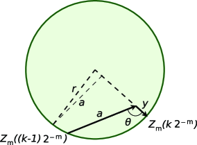
Figure 9: Illustration of the geometry underlying the argument of Lemma 19.

First note that $|Z_{m}(k2^{-m})-Z_{m}((k-1)2^{-m})|=\sqrt{a^{2}+y^{2}-2ay\cos\theta}$(where we abuse notation by letting $y$ also stand for the length of the vector $y$). This increases as $\theta$ increases to $\pi$, so long as $a$, $y$, $Z_{m}(k2^{-m})$ are held fixed. Thus we can assume that $\theta$ has increased to the point where $Z_{m}((k-1)2^{-m})$, as well as $Z_{m}(k2^{-m})$, belong to $\partial B$. (This will happen if, as required above, $2^{-m}<r$.) Now observe that the distance $|Z_{m}(k2^{-m})-Z_{m}((k-1)2^{-m})|$ will be bounded above by the smaller of the two distances from $Z_{m}(k2^{-m})$ to the intercepts of $\partial B$ by a line parallel to $y$, and at distance $a$ from $Z_{m}(k2^{-m})$. But two applications of Pythagoras’ theorem show that this distance is given by

$$\sqrt{a^{2}+\bigl{(}r-\sqrt{r^{2}-a^{2}}\bigr{)}^{2}} = \sqrt{2r^{2}-2r\sqrt{r^{2}-a^{2}}}$$

$$= \sqrt{2}r\sqrt{1-\sqrt{1-\frac{a^{2}}{r^{2}}}}=\sqrt{2}r\sqrt{\frac{a^{2}}{2r^{2}}\biggl{(}1+\frac{1}{4}(z^{*})^{2}\biggr{)}}$$

for some $z^{*}$ in the range $[0,\frac{r^{2}}{a^{2}}]$. (The last step arises from a second-order Taylor series expansion.) Therefore

$$\sqrt{a^{2}+\bigl{(}r-\sqrt{r^{2}-a^{2}}\bigr{)}^{2}}\leq\sqrt{2}r\sqrt{\frac{a^{2}}{2r^{2}}\biggl{(}1+\frac{a^{2}}{4r^{2}}\biggr{)}}\leq a\biggl{(}1+\frac{a^{2}}{8r^{2}}\biggr{)}$$

(using $\sqrt{1+z}\leq 1+\frac{1}{2}z$ for $z\geq-1$).

Thus the total path length over the time interval $(s,t)$ is bounded above by

$$\bigl{(}(t-s)2^{m}+2\bigr{)}\times 2^{-m}\biggl{(}1+\frac{2^{-2m}}{8r^{2}}\biggr{)},$$

which converges to $t-s$ as $m\to\infty$. Hence we obtain

$$\operatorname{dist}_{\mathrm{intr}}(Z(s),Z(t))\leq t-s,$$

thus establishing the $\operatorname{Lip}(1)$ property in intrinsic metric for $Z$.

We will show that the bound in Proposition 18 is uniform over all $X(0)$ and $Y(0)$. We will switch from the intrinsic distance to the Euclidean distance in the formulation of the next proposition. This is legitimate in view of (10).

Proposition 20

Let $D$ be a domain satisfying uniform exterior sphere and interior cone conditions. Suppose that there exist $t_{1}>0$ and $\varepsilon_{1}>0$ such that, for any $X$ and $Y$ satisfying (35) and (36) with $X(0)$, $Y(0)\in\overline{D}$,

$$\mathbb{P}\Bigl{[}\inf_{0\leq t\leq t_{1}}|X(t)-Y(t)|\leq\varepsilon_{1}\Bigr{]}>0.$$ (50)

Then

$$\mathbb{P}\Bigl{[}\inf_{0\leq t\leq t_{1}}|X(t)-Y(t)|\leq\varepsilon_{1}\Bigr{]}>p_{1}$$ (51)

for some $p_{1}>0$ not depending on $X(0)$ and $Y(0)$.

Suppose (51) does not hold. Then there exist $t_{1}>0$, $\varepsilon_{1}>0$, sequences $\{x_{n}\}_{n\geq 1}$, $\{y_{n}\}_{n\geq 1}$ of points in $\overline{D}$, random processes $\{A_{t},t\geq 0\}$, $\{B_{t},t\geq 0\}$, $\{\mathbb{J}^{n}_{t},t\geq 0\}$ and $\{\mathbb{K}^{n}_{t},t\geq 0\}$, and solutions $X^{n}$ and $Y^{n}$ of (35) and (36) satisfying the following properties. The processes $A$ and $B$ are $d$-dimensional Brownian motions starting from 0, and independent of each other. The $(d\times d)$-matrix-valued processes $\mathbb{J}^{n}$ and $\mathbb{K}^{n}$ are predictable with respect to the natural filtration of $A$ and $B$, such that $(\mathbb{J}^{n}_{t})^{\top}\mathbb{J}_{t}^{n}+(\mathbb{K}^{n}_{t})^{\top}\mathbb{K}_{t}$ is the $(d\times d)$ identity matrix at all times $t$. Let $X^{n}$ and $Y^{n}$ denote solutions to (35) and (36) based on the Brownian motions $A$ and $B$, using the predictable integrators $\mathbb{J}^{n}$ and $\mathbb{K}^{n}$, and starting from $X^{n}(0)=x_{n}\in\overline{D}$ and $Y^{n}(0)=\break y_{n}\in\overline{D}$. Then

$$\mathbb{P}\Bigl{[}\inf_{0\leq t\leq t_{1}}|X^{n}(t)-Y^{n}(t)|>\varepsilon_{1}\Bigr{]}>1-2^{-n}.$$ (52)

Let $(M^{n,1}_{t},M^{n,2}_{t})=(\int_{0}^{t}\,\mathrm{d}B_{s},\int_{0}^{t}(\mathbb{J}^{n}_{s})^{\top}\,\mathrm{d}B_{s}+\int_{0}^{t}(\mathbb{K}^{n}_{s})^{\top}\,\mathrm{d}A_{s})$. The processes $M^{n,1}$ and $M^{n,2}$ are Brownian motions and so the sequence of pairs is tight, which therefore possesses a subsequence converging in distribution. By abuse of notation, we assume that the whole sequence $(M^{n,1},M^{n,2})$ converges in distribution to, say, $(M^{\infty,1},M^{\infty,2})$. It is clear that $M^{\infty,1}$ and $M^{\infty,2}$ are Brownian motions.

Let $\mathcal{F}_{t}=\sigma((M^{\infty,1}_{s},M^{\infty,2}_{s}),s\leq t)$ be the natural filtration for $(M^{\infty,1},M^{\infty,2})$. We will show that $(M^{\infty,1},M^{\infty,2})$ are co-adapted Brownian motions relative to $\{\mathcal{F}_{t}\}$. Since $(M^{n,1},M^{n,2})$ are co-adapted Brownian motions, for all $0\leq t_{1}\leq t_{2}\leq\cdots\leq t_{n}\leq t\leq s_{1}\leq s_{2}$, the random variable $M^{n,1}_{s_{2}}-M^{n,1}_{s_{1}}$ is independent of

$$((M^{n,1}_{t_{1}},M^{n,2}_{t_{1}}),(M^{n,1}_{t_{2}},M^{n,2}_{t_{2}}),\ldots,(M^{n,1}_{t_{n}},M^{n,2}_{t_{n}})).$$

Independence is preserved by weak limits, so $M^{\infty,1}_{s_{2}}-M^{\infty,1}_{s_{1}}$ is independent of

$$((M^{\infty,1}_{t_{1}},M^{\infty,2}_{t_{1}}),(M^{\infty,1}_{t_{2}},M^{\infty,2}_{t_{2}}),\ldots,(M^{\infty,1}_{t_{n}},M^{\infty,2}_{t_{n}})).$$

This implies that $M^{\infty,1}_{s_{2}}-M^{\infty,1}_{s_{1}}$ is independent of $\mathcal{F}_{t}$. Since the same argument applies to $M^{\infty,2}_{s_{2}}-M^{\infty,2}_{s_{1}}$, we see that $(M^{\infty,1},M^{\infty,2})$ are co-adapted relative to $\{\mathcal{F}_{t}\}$. Recall from Section 1.2 that this implies that there exist Brownian motions $\{A^{\infty}_{t},t\geq 0\}$ and $\{B^{\infty}_{t},t\geq 0\}$ and processes $\{\mathbb{J}^{\infty}_{t},t\geq 0\}$ and $\{\mathbb{K}^{\infty}_{t},t\geq 0\}$ such that $(M^{\infty,1}_{t},M^{\infty,2}_{t})=(\int_{0}^{t}\,\mathrm{d}B^{\infty}_{s},\int_{0}^{t}(\mathbb{J}^{\infty}_{s})^{\top}\,\mathrm{d}B^{\infty}_{s}+\int_{0}^{t}(\mathbb{K}^{\infty}_{s})^{\top}\,\mathrm{d}A^{\infty}_{s})$.

Recall that $(M^{n,1},M^{n,2})\to(M^{\infty,1},M^{\infty,2})$ weakly in the uniform topology on all compact intervals. Going back to the original notation, we see that

$$\biggl{(}\int_{0}^{t}\,\mathrm{d}B_{s},\int_{0}^{t}(\mathbb{J}^{n}_{s})^{\top}\,\mathrm{d}B_{s}+\int_{0}^{t}(\mathbb{K}^{n}_{s})^{\top}\,\mathrm{d}A_{s}\biggr{)}$$

$$\qquad\to\biggl{(}\int_{0}^{t}\,\mathrm{d}B^{\infty}_{s},\int_{0}^{t}(\mathbb{J}^{\infty}_{s})^{\top}\,\mathrm{d}B^{\infty}_{s}+\int_{0}^{t}(\mathbb{K}^{\infty}_{s})^{\top}\,\mathrm{d}A^{\infty}_{s}\biggr{)}$$

weakly in the uniform topology on all compact intervals. By the Skorokhod lemma, we can assume that the processes converge a.s. in the supremum topology on compact intervals.

Since $\overline{D}$ is compact, we can assume, passing to a subsequence if necessary, that the initial points satisfy $x_{n}\to x_{\infty}\in\overline{D}$ and $y_{n}\to y_{\infty}\in\overline{D}$ as $n\to\infty$. In view of the representation of coupled reflected Brownian motions using stochastic differential equations (35) and (36), established in Saisho [(1987), Theorem 4.1], and employing the continuous dependence on driving Brownian motions established there, we see that $(X^{n},Y^{n})\to(X^{\infty},Y^{\infty})$ weakly in the uniform topology on all compact intervals, where $(X^{\infty},Y^{\infty})$ represents the solution to (35) and (36) with $X^{\infty}(0)=x_{\infty}$, $Y^{\infty}(0)=y_{\infty}$, corresponding to $A^{\infty}$, $B^{\infty}$, $\mathbb{J}^{\infty}$ and $\mathbb{K}^{\infty}$. We obtain from (52) and weak convergence of $(X^{n},Y^{n})$ to $(X^{\infty},Y^{\infty})$ that, for every $n$,

$$\mathbb{P}\Bigl{[}\inf_{0\leq t\leq t_{1}}|X^{\infty}(t)-Y^{\infty}(t)|\geq\varepsilon_{1}\Bigr{]}\geq 1-2^{-n}.$$

Taking the limit as $n\to\infty$, this contradicts (50) in the statement of the Proposition. Consequently (51) must hold for some $p_{1}$.

We now complete the proof of Theorem 1, applying Proposition 20 together with standard reasoning. Consider processes $X$ and $Y$ starting from any pair of points in $\overline{D}$ and corresponding to any “strategy” $\mathbb{J}$ and $\mathbb{K}$. Because of the uniform bound in Proposition 20, the probability of $X$ and $Y$ not coming within distance $\varepsilon_{1}$ of each other on the interval $[kt_{1},(k+1)t_{1}]$, conditional on not coming within this distance before $kt_{1}$, is bounded above by $1-p_{1}$ for any $k$, by the Markov property. Hence, the probability of $X$ and $Y$ not coming within distance $\varepsilon_{1}$ of each other on the interval $[0,kt_{1}]$ is bounded above by $(1-p_{1})^{k}$. Letting $k\to\infty$, it follows that $X$ and $Y$ are not $\varepsilon_{1}$-shy. Since $\varepsilon_{1}$ can be taken arbitrarily small, the proof of Theorem 1 is complete.

We remark that the matrices $\mathbb{J}$ and $\mathbb{K}$ employed in (35) and (36) are predictable and, consequently, the choice of the pursuer’s velocity is based strictly on past information. This is in contrast to the pursuit–evasion problems and associated paradoxes discussed by Bollobas, Leader and Walters (2012).

5 Complements and conclusions.

We conclude this paper by remarking on some supplementary results and concepts, and by considering possibilities for future work.

5.1 Comparison with previous methods.

The fundamental idea in this paper turns out in the end to resemble that of Benjamini, Burdzy and Chen (2007), but uses simple notions of weak convergence and tightness, rather than detailed large deviation estimates. Moreover, the use of metric geometry notions enables us to finesse many analytical technicalities. (Perhaps this is the first application of modern metric geometry to Euclidean stochastic calculus?) On the other hand, the stochastic control methods of Kendall (2009) are quite different. The stochastic control approach uses potential theory to estimate the value function of an associated stochastic game; consequently the methods of Kendall (2009) may be expected to give sharper information (bounds on expectation of stopping times), but in more limited cases (convexity of domain). However, one can observe that, at least in principle, the stochastic game formulation still applies in the general case. For example, there is a value function to be discovered for a stochastic control reformulation of Theorem 1, and in principle it might be possible to estimate this value function and so gain more information than is supplied by the weak geometric bounds established above.

We note that many promising ideas based on stochastic calculus fail to show nonshyness because they cannot be applied to “perverse” couplings with the property that, on some time intervals, $|X-Y|$ grows at a deterministic rate [see Example 4.2 of Benjamini, Burdzy and Chen (2007)].

Also note that the proof in Kendall (2009), which works in convex domains, does not appear to be (directly) extendable to calculations involving the intrinsic metric—simple manipulation using symbolic Itô calculus [Kendall (2001)] shows that the drift of $\operatorname{dist}_{\mathrm{intr}}(X,Y)$ is unbounded at distances bounded away from zero. In particular, Bessel-like divergences for $\operatorname{dist}_{\mathrm{intr}}(X,Y)$ of magnitude $a$ occur when the geodesic from $X$ to $Y$ touches a concave part of $\partial D$ at $x$ and $|x-Y|=1/a$. The first-order differential geometry given in Proposition 14 (the generalization of Gauss’ lemma) is the best we can do for $\operatorname{CAT}({0})$ domains satisfying uniform exterior sphere and interior cone conditions.

5.2 Higher dimensions and the failure of $\operatorname{CAT}({0})$.

For planar domains, $\operatorname{CAT}({0})$ and simple-connectedness are equivalent, in which case, by Theorem 2, there are no shy co-adapted couplings. In higher dimensions, it is natural to ask whether the $\operatorname{CAT}({0})$ condition is essential for there to be no shy coupling. We do not at all believe this to be the case. It is possible to give an argument suggesting that star-shaped domains with smooth boundary conditions cannot support shy couplings, by establishing the analogous result for a corresponding deterministic pursuit–evasion problem. To apply this argument to the probabilistic case would require more careful arguments. We therefore leave this as a project for another day.

As a spur to future work, we formulate a bold and possibly rash conjecture:

Conjecture 1.

There can be no shy co-adapted coupling for reflecting Brownian motions in bounded contractible domains in any dimension.

While resolution of the star-shaped case appears to be largely a technical matter, we believe that new ideas will be required to make substantial progress toward resolving the conjecture.

5.3 When can shyness exist?

Many examples of shy couplings can be generated using suitable symmetries. However, we do not know of any examples in which symmetries play no rôle. Accordingly we formulate a further conjecture:

Conjecture 2.

If a bounded domain $D$ supports a shy co-adapted coupling for reflecting Brownian motions, then there exists a shy co-adapted coupling that can be realized using a rigid-motion symmetry of the domain $D$.

A stronger form of the above conjecture, saying “If a bounded domain $D$ supports a shy co-adapted coupling for reflecting Brownian motions, then the shy coupling is realized using a rigid-motion symmetry of the domain $D$,” is false. To see this, consider the planar annulus $A=\mathcal{B}(0,2)\setminus\mathcal{B}(0,1)$ and let $\mathcal{T}$ be the symmetry with respect the origin. Let $X$ be reflected Brownian motion in $A$ and $Y=\mathcal{T}(X)$. Let $D=A\times(0,1)$ and let $Z$ be reflected Brownian motion in $(0,1)$, independent of $X$ and $Y$. Then $(X,Z)$ and $(Y,Z)$ form a shy coupling in $D$ which cannot be realized using a rigid-motion symmetry of $D$.

Note that Benjamini, Burdzy and Chen [(2007), Example 3.9] supplies an example based on Brownian motion on graphs, for which there is no fixed-point-free isometry and yet a shy coupling exists. However we do not see how to use the idea of this construction to construct a counterexample to the above conjecture.

5.4 Further questions.

We enumerate a short list of additional questions. [(1)]

Shyness is interesting for foundational reasons: coupling is an important tool in probability, and shyness informs us about coupling. We do not know of any honest applications of shyness. However, one can contrive a kind of cryptographic context. Suppose one wishes to mimic a target $Y$, which is a randomly evolving high-dimensional structure, in such a way that the mimic $X$ never comes within a certain distance of the target $Y$. Shyness concerns the question, whether it is possible to do this in a way that is perfectly concealed from an observer watching the mimic $X$ alone.

In this formulation, it is not clear why one should restrict consideration to co-adapted couplings. Our methods do not lend themselves to the non-co-adapted case, and the question is open whether or not results change substantially if one is allowed to use such couplings. In particular, it seems possible that Conjecture 2 might have a quite different answer in this context.

In further work [Bramson, Burdzy and Kendall (2011)] we plan to study the deterministic pursuit–evasion problem, in conjunction with shy couplings, for multidimensional $\operatorname{CAT}({\kappa})$ domains possessing “stable rubber bands,” a condition that is partly topological and partly geometric. As a corollary, we plan to prove that there are no shy couplings in multidimensional star-shaped domains.

The Lion and Man problem has been generalized to the case of multiple Lions. [An early instance is given in Croft (1964).] Can one formulate and prove useful results for a corresponding notion of multiple shyness?

References

- Alexander, Bishop and Ghrist (2006) {bmisc}[auto:STB—2012/03/21—07:41:58] \bauthor\bsnmAlexander, \bfnmS.\binitsS., \bauthor\bsnmBishop, \bfnmR. L.\binitsR. L. and \bauthor\bsnmGhrist, \bfnmR.\binitsR. (\byear2006). \bhowpublishedPursuit and evasion in non-convex domains of arbitrary dimension. In Proceedings of Robotics: Science and Systems, Philadelphia, USA. \bptokimsref \endbibitem
- Alexander, Bishop and Ghrist (2010) {barticle}[mr] \bauthor\bsnmAlexander, \bfnmS.\binitsS., \bauthor\bsnmBishop, \bfnmR.\binitsR. and \bauthor\bsnmGhrist, \bfnmR.\binitsR. (\byear2010). \btitleTotal curvature and simple pursuit on domains of curvature bounded above. \bjournalGeom. Dedicata \bvolume149 \bpages275–290. \biddoi=10.1007/s10711-010-9481-z, issn=0046-5755, mr=2737693 \bptokimsref \endbibitem