Variational methods with coupled Gaussian functions for Bose-Einstein condensates with long-range interactions. II. Applications

Abstract

Bose-Einstein condensates with an attractive $1/r$ interaction and with dipole-dipole interaction are investigated in the framework of the Gaussian variational ansatz introduced by S. Rau, J. Main, and G. Wunner [Phys. Rev. A, submitted]. We demonstrate that the method of coupled Gaussian wave packets is a full-fledged alternative to direct numerical solutions of the Gross-Pitaevskii equation, or even superior in that coupled Gaussians are capable of producing both, stable and unstable states of the Gross-Pitaevskii equation, and thus of giving access to yet unexplored regions of the space of solutions of the Gross-Pitaevskii equation. As an alternative to numerical solutions of the Bogoliubov-de Gennes equations, the stability of the stationary condensate wave functions is investigated by analyzing the stability properties of the dynamical equations of motion for the Gaussian variational parameters in the local vicinity of the stationary fixed points. For blood-cell-shaped dipolar condensates it is shown that on the route to collapse the condensate passes through a pitchfork bifurcation, where the ground state itself turns unstable, before it finally vanishes in a tangent bifurcation.

I Introduction

In the previous paper paper1 variational methods with coupled Gaussian functions for Bose-Einstein condensates with long-range interactions have been developed. The purpose of this paper is to demonstrate the power of this approach by applying the variational methods to two different types of condensates, viz. a monopolar condensate with an attractive gravity-like $1/r$ interaction and a dipolar condensate.

Monopolar condensates with an attractive $1/r$ interaction, originally proposed by O’Dell et al. ODellPRL84 , have unique stability properties. For a wide range of the scattering length the condensate is stable without an external trap. Additionally, the gravity-like interaction of a monopolar condensate may be an opportunity to investigate usually large-scale physical properties like, e.g., boson stars RuffiniPhysRev187 at a laboratory scale. The “monopolar” interaction of two neutral atoms with positions $\bm{r}$ and $\bm{r}^{\prime}$ is induced by the presence of external electromagnetic radiation. O’Dell et al. ODellPRL84 suggest six triads of orthogonal laser beams to induce the interatomic potential $W_{\mathrm{lr}}(\bm{r},\bm{r}^{\prime})=-u/|\bm{r}-\bm{r}^{\prime}|$, where $u$ depends on the intensity and wave vector of the radiation, and on the isotropic polarizability of the atoms. Although this system has not yet been realized experimentally it has already served as a model to compare results obtained analytically and with exact numerical techniques PapadopoulosPRA76 ; holgerPRA77 ; holgerPRA78 .

By contrast, Bose-Einstein condensates with a long-range dipole-dipole interaction $W_{\mathrm{lr}}(\bm{r},\bm{r}^{\prime})\sim(1-3\cos^{2}\theta)|\bm{r}-\bm{r}^{\prime}|^{-3}$ have been obtained experimentally with ${}^{52}\mathrm{Cr}$ atoms in 2005 by Griesmaier et al. EXGriesmaierPRL94 ; EXStuhlerPRL95 , and more recently in 2008 by Beaufils et al. BeaufilsPRA77 . The collapse of the condensate also has been subject to extensive experimental studies Koch08Nature . Theoretical investigations have so far mostly been based on lattice simulations Ronen ; Ronen06a ; WilsonPRA80 or on a simple variational approach with a Gaussian type orbital gelbPatrick . For a review on dipolar condensates see Lahaye2009 .

In this paper we extend and elaborate in more detail preliminary work presented in Rau10 . In Sec. II the results for the monopolar condensates are presented and discussed. It is shown that only three to five coupled Gaussians are sufficient to achieve convergence of the mean-field energy, the chemical potential, and the lowest eigenvalues of the stability matrix. In Sec. III the method of coupled Gaussians is applied to dipolar BEC to clarify the theoretical nature of the collapse mechanism of blood-cell shaped condensates. On the route to collapse the condensates passes through a pitchfork bifurcation, where the ground state itself turns unstable, before it finally vanishes in a tangent bifurcation. Conclusions are drawn in Sec. IV.

II Monopolar Condensates

The time-independent Gross-Pitaevskii equation (GPE) for a self-trapped condensate with a short-range contact interaction with scattering length $a$ and a long-range monopolar interaction reads

$$\bigg{[}-\Delta+8\pi N\frac{a}{a_{u}}\left|\psi(\bm{r})\right|^{2}-2N\int\mathrm{d}^{3}\bm{r}^{\prime}\frac{\left|\psi(\bm{r}^{\prime})\right|^{2}}{\left|\bm{r}-\bm{r}^{\prime}\right|} \bigg{]}\psi(\bm{r})$$

$$=\mu \psi(\bm{r})\;,$$ (1)

where the natural “atomic” units introduced in Ref. PapadopoulosPRA76 were used. Lengths are measured in units of a “Bohr radius” $a_{u}=\hbar^{2}/(mu)$, energies in units of a “Rydberg energy” $E_{u}=\hbar^{2}/(2ma_{u}^{2})$, and times in units of $t_{u}=\hbar/E_{u}$, where $u$ determines the strength of the atom-atom-interaction ODellPRL84 , and $m$ is the mass of one boson. The number of bosons $N$ can be eliminated from Eq. (1) by using scaling properties of the system PapadopoulosPRA76 ; holgerPRA78 . We define $\bm{r}=\tilde{\bm{r}}/N$, $\psi=N^{3/2}\tilde{\psi}$, which leaves the norm of the wave function invariant, $a_{\mathrm{sc}}=N^{2}a/a_{u}$, $\tilde{\mu}=\mu/N^{2}$, omit the tilde in what follows, substitute $\mu\to\mathrm{i}(\mathrm{d}/\mathrm{d}t)$, and finally obtain the time-dependent GPE in scaled “atomic” units

$$\bigg{[} -\Delta+8\pi a_{\mathrm{sc}}\left|\psi(\bm{r},t)\right|^{2}$$

$$-2\int\mathrm{d}^{3}\bm{r}^{\prime}\frac{\left|\psi(\bm{r}^{\prime},t)\right|^{2}}{\left|\bm{r}-\bm{r}^{\prime}\right|}\bigg{]}\psi(\bm{r},t)=\mathrm{i}\frac{\mathrm{d}}{\mathrm{d}t}\psi(\bm{r},t)\;.$$ (2)

It is known that for Bose-Einstein condensates with attractive $1/r$ interaction two real radially symmetric solutions, the ground state and a collectively excited state, exist. By varying the scattering length $a_{\mathrm{sc}}$, they are created in a tangent bifurcation at a critical value of $a_{\mathrm{sc}}$ PapadopoulosPRA76 ; holgerPRA77 ; holgerPRA78 . Below the tangent bifurcation no stationary solutions exist. Approaching the bifurcation point from higher scattering lengths the condensate collapses. A similar behavior is found for dipolar condensates gelbPatrick and condensates without long-range interactions HuepePRA .

For the monopolar GPE numerically exact solutions exist. The numerical procedure for the direct integration of the GPE is introduced in Refs. PapadopoulosPRA76 ; holgerPRA77 ; holgerPRA78 . It is our purpose to investigate the two states connected via the tangent bifurcation with the coupled Gaussian wave packet method. We use the ansatz

$$\psi(r)=\sum_{k=1}^{N}\mathrm{e}^{\mathrm{i}(a^{k}r^{2}+\gamma^{k})}=\sum_{k=1}^{N}g^{k}$$ (3)

for condensates with spherical symmetry. Following the procedure outlined in paper1 the dynamical equations for the variational parameters read

$$\dot{\gamma}^{k} =6\mathrm{i}a^{k}-v_{0}^{k}\;,$$ (4a)

$$\dot{a}^{k} =-4(a^{k})^{2}-\frac{1}{2}V_{2}^{k}\;,$$ (4b)

for $k=1,\dots,N$. The quantities $v_{0}^{k}$ and $V_{2}^{k}$ are obtained from the $(2N\times 2N)$-dimensional linear set of equations ($k,l=1,\dots,N$)

$$\begin{pmatrix}(1)_{kl}&(r^{2})_{kl}\\[2.15277pt] (r^{2})_{lk}&(r^{4})_{kl}\end{pmatrix}\begin{pmatrix}v_{0}^{k}\\[2.15277pt] \frac{1}{2}V_{2}^{k}\end{pmatrix}=\sum_{k=1}^{N}\begin{pmatrix}\langle g^{l}|V_{\rm{eff}}|g^{k}\rangle\\[4.30554pt] \langle g^{l}|r^{2}V_{\rm{eff}}|g^{k}\rangle\end{pmatrix},$$ (5)

where $V_{\mathrm{eff}}=V_{\mathrm{sc}}+V_{\mathrm{m}}$ is the sum of the contact and monopolar potential, and the matrix elements read

$$\left(1\right)_{lk}:\bigl{<}g^{l}\big{|}g^{k}\bigr{>}=\pi^{\nicefrac{{3}}{{2}}}\dfrac{\mathrm{e}^{\mathrm{i}\gamma^{kl}}}{\left(-\mathrm{i}a^{kl}\right)^{\nicefrac{{3}}{{2}}}}\;,$$ (6a)

$$\left(r^{2}\right)_{lk}:\bigl{<}g^{l}\bigl{|}r^{2}\bigr{|}g^{k}\bigr{>}=\dfrac{3}{2}\pi^{\nicefrac{{3}}{{2}}}\dfrac{\mathrm{e}^{\mathrm{i}\gamma^{kl}}}{\left(-\mathrm{i}a^{kl}\right)^{\nicefrac{{5}}{{2}}}}\;,$$ (6b)

$$\left(r^{4}\right)_{lk}:\bigl{<}g^{l}\bigl{|}r^{4}\bigr{|}g^{k}\bigr{>}=\dfrac{15}{4}\pi^{\nicefrac{{3}}{{2}}}\dfrac{\mathrm{e}^{\mathrm{i}\gamma^{kl}}}{\left(-\mathrm{i}a^{kl}\right)^{\nicefrac{{7}}{{2}}}}\;,$$ (6c)

$$\bigl{<}g^{l}\bigl{|}V_{\mathrm{sc}}\bigr{|}g^{k}\bigr{>}=\sum_{i,j=1}^{N}8a_{\mathrm{sc}}\pi^{\nicefrac{{5}}{{2}}}\dfrac{\mathrm{e}^{\mathrm{i}\gamma^{klij}}}{\left(-\mathrm{i}a^{klij}\right)^{\nicefrac{{3}}{{2}}}}\;,$$ (6d)

$$\bigl{<}g^{l}\bigl{|}V_{\mathrm{m}}\bigr{|}g^{k}\bigr{>}=4\sum_{i,j=1}^{N}\pi^{\nicefrac{{5}}{{2}}}\dfrac{\mathrm{e}^{\mathrm{i}{\gamma^{klij}}}}{a^{ij}a^{kl}\sqrt{-\mathrm{i}a^{klij}}}\;,$$ (6e)

$$\bigl{<}g^{l}\bigl{|}r^{2}V_{\mathrm{sc}}\bigr{|}g^{k}\bigr{>}=12\sum_{i,j=1}^{N}a_{\mathrm{sc}}\pi^{\nicefrac{{5}}{{2}}}\dfrac{\mathrm{e}^{\mathrm{i}\gamma^{klij}}}{\left(-\mathrm{i}a^{klij}\right)^{\nicefrac{{5}}{{2}}}}\;,$$ (6f)

$$\bigl{<}g^{l}\bigl{|}r^{2}V_{\mathrm{m}}\bigr{|}g^{k}\bigr{>}=2\sum_{i,j=1}^{N}\pi^{\nicefrac{{5}}{{2}}}\dfrac{\mathrm{e}^{\mathrm{i}{\gamma^{klij}}}\left(2a^{ij}+3a^{kl}\right)}{a^{ij}\left(a^{kl}\right)^{2}\left(-\mathrm{i}a^{klij}\right)^{\nicefrac{{3}}{{2}}}}\;,$$ (6g)

with the abbreviations

$$a^{kl}=a^{k}-\left(a^{l}\right)^{*}\;,\quad a^{ij}=a^{i}-\left(a^{j}\right)^{*}\;,$$ (7a)

$$\gamma^{kl}=\gamma^{k}-\left(\gamma^{l}\right)^{*}\;,\quad\gamma^{ij}=\gamma^{i}-\left(\gamma^{j}\right)^{*}\;,$$ (7b)

$$a^{klij}=a^{kl}+a^{ij}\;,\quad\gamma^{klij}=\gamma^{kl}+\gamma^{ij}\;.$$ (7c)

II.1 Stationary solutions

Stationary solutions of the GPE can be computed via a nonlinear root search of the dynamical equations (4) as outlined in paper1 . The Gaussian parameters obtained from the root search are then used to calculate the mean field energy

$$E_{\rm mf} =\sum_{k,l=1}^{N}2\pi^{\nicefrac{{3}}{{2}}}\mathrm{e}^{\mathrm{i}\gamma^{kl}}\Biggl{[}-3\frac{a^{k}\left(a^{l}\right)^{*}}{\left(a^{kl}\right)^{2}\sqrt{-\mathrm{i}a^{kl}}}$$

$$+\sum_{i,j=1}^{N}\frac{\pi\mathrm{e}^{\mathrm{i}\gamma^{ij}}}{\sqrt{-\mathrm{i}a^{klij}}}\left(\frac{2a_{\mathrm{sc}}}{-\mathrm{i}a^{klij}}+\frac{1}{a^{ij}a^{kl}}\right)\Biggr{]}$$ (8)

and the chemical potential

$$\mu =\sum_{k,l=1}^{N}2\pi^{\nicefrac{{3}}{{2}}}\mathrm{e}^{\mathrm{i}\gamma^{kl}}\Biggl{[}-3\frac{a^{k}\left(a^{l}\right)^{*}}{\left(a^{kl}\right)^{2}\sqrt{-\mathrm{i}a^{kl}}}$$

$$+\sum_{i,j=1}^{N}\frac{\pi\mathrm{e}^{\mathrm{i}\gamma^{ij}}}{\sqrt{-\mathrm{i}a^{klij}}}\left(\frac{4a_{\mathrm{sc}}}{-\mathrm{i}a^{klij}}+\frac{2}{a^{ij}a^{kl}}\right)\Biggr{]}\;.$$ (9)

For the variational ansatz with only one single Gaussian function ($N=1$) the results can be obtained analytically holgerPRA77 ; holgerPRA78 , viz.

$$E_{\mathrm{mf}}^{N=1}=-\frac{4}{9\pi}\frac{1\pm 2\sqrt{1+\frac{8a_{\mathrm{sc}}}{3\pi}}}{\left(1\pm\sqrt{1+\frac{8a_{\mathrm{sc}}}{3\pi}}\right)^{2}}$$ (10)

for the mean field energy, and

$$\mu^{N=1}=-\frac{4}{9\pi}\frac{5\pm 4\sqrt{1+\frac{8a_{\mathrm{sc}}}{3\pi}}}{\left(1\pm\sqrt{1+\frac{8a_{\mathrm{sc}}}{3\pi}}\right)^{2}}$$ (11)

for the chemical potential.

The results of the variational computations with $N=1$ to $N=5$ coupled Gaussian functions are presented in Fig. 1(a) for the mean field energy and in (b) for the chemical potential.

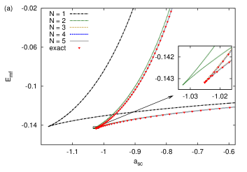
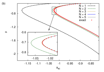
Figure 1: (a) Mean field energy $E_{\mathrm{mf}}$ for self-trapped condensates with attractive $1/r$ interaction as a function of the scattering length obtained by using up to five coupled Gaussian wave packets ($N=1,\dots,5$, respectively) in comparison with the result of the accurate numerical solution of the stationary Gross-Pitaevskii equation (exact). (b) Same as (a) but for the chemical potential $\mu$.

For comparison the results of the exact solution obtained by direct numerical integration of the GPE are shown as red triangles. Although the variational solution with a single Gaussian significantly differs from the exact calculation, the qualitative behavior is the same: two solutions emerge in a tangent bifurcation at a critical scattering length, which is $a_{\mathrm{sc}}^{\mathrm{cr,v}}=-3\pi/8=-1.178097$ and $a_{\mathrm{sc}}^{\mathrm{cr,n}}=-1.025147$ for the variational and exact calculation, respectively PapadopoulosPRA76 . Note that the excited state with higher mean field energy has a lower chemical potential than the ground state.

The main purpose of Fig. 1 is to demonstrate how the coupling of only $N=2$ to $N=5$ Gaussian functions drastically improves the results obtained with a simple Gaussian type orbital. The coupling of only two Gaussian functions already leads to a significant improvement for both, the mean field energy value and the chemical potential. For three or more coupled Gaussians, the results in Fig. 1 can no longer be distinguished from the numerically exact solution. The enlargements in Fig. 1 illustrate the rapid convergence of the results with increasing number $N$ of coupled Gaussians.

Detailed values for the mean field energy and the chemical potential of the ground state and the excited state at scattering length $a_{\mathrm{sc}}=-1$ close to the tangent bifurcation are presented in Table 1.

Table 1: Dependence of the critical scattering length $a_{\mathrm{sc}}^{\mathrm{cr}}$ of the tangent bifurcation and the mean field energy and the chemical potential of the ground state (g) and the excited state (e) at scattering length $a_{\mathrm{sc}}=-1$ on the number $N$ of coupled Gaussian functions.

$N$	$a_{\mathrm{sc}}^{\mathrm{cr}}$	$E_{\rm mf}^{\rm g}$	$\mu^{\rm g}$	$E_{\rm mf}^{\rm e}$	$\mu^{\rm e}$
$1$	$-1.178097$	$-0.130383$	$-0.480807$	$-0.084219$	$-1.304592$
$2$	$-1.032780$	$-0.140151$	$-0.584799$	$-0.136826$	$-0.892376$
$3$	$-1.025527$	$-0.140637$	$-0.595154$	$-0.138380$	$-0.862562$
$4$	$-1.025167$	$-0.140655$	$-0.595659$	$-0.138449$	$-0.860862$
$5$	$-1.025149$	$-0.140656$	$-0.595682$	$-0.138452$	$-0.860767$
$\infty$	$-1.025147$	$-0.140657$	$-0.595685$	$-0.138453$	$-0.860757$

The coupling of three Gaussian functions already yields an accuracy of more than four digits for the mean field energy of the ground state. Using up to five Gaussians, we can safely assume the variational result as to be fully converged to the exact numerical computation marked as $N=\infty$. The rapid convergence of the critical scattering length $a_{\mathrm{sc}}^{\mathrm{cr}}$ with increasing number of coupled Gaussians is also illustrated in Table 1.

In previous work PapadopoulosPRA76 it has been noted that the peak amplitude of the exact wave function at the center $r=0$ is poorly reproduced by a Gaussian type orbital. Here, we illustrate that superpositions of Gaussian functions can accurately approximate the exact wave function and thus also provide the correct peak amplitude.

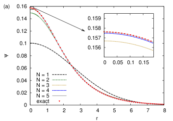
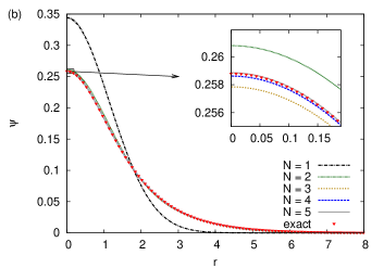
Figure 2: Wave function $\psi(r)$ of (a) the stable ground state, (b) the excited state, at scattering length $a_{\mathrm{sc}}=-1$ close to the exact numerical bifurcation. The calculations with coupled Gaussians converge rapidly to the exact numerical wave function (triangles).

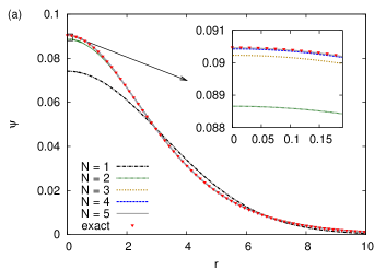
Figure 3: Same as Fig. 2 but at scattering length $a_{\mathrm{sc}}=-0.6$.

In Fig. 2 we choose the scattering length $a_{\mathrm{sc}}=-1$ close to the exact numerical bifurcation at $a_{\mathrm{sc}}^{\mathrm{cr}}=-1.02515$ to compare the wave function of the variational and the numerically exact ground and excited state. As a second example, we choose $a_{\mathrm{sc}}=-0.6$ in Fig. 3, which lies farther away from the critical scattering length. The rapid convergence of the variational wave functions with the number of Gaussians increasing from $N=1$ to 5 is impressive as can be seen in the insets in Figs. 2 and 3. Note that far from the bifurcation the wave function of the stable state in Fig. 3(a) and the wave function of the excited state in Fig. 3(b) differ greatly, while for $a_{\mathrm{sc}}=-1$ both wave functions in Fig. 2(a) and (b) are similar. At the tangent bifurcation, both merging states, the stable ground state and the excited state are described by the same wave function. The reason is that due to the nonlinearity of the GPE, the solution at the tangent bifurcation has the properties of an “exceptional point” holgerPRA77 .

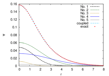
Figure 4: The constituents of the five-Gaussian ansatz (No. 1, $\ldots$, 5) plotted separately. The superposition of the five Gaussians (coupled), excellently agrees with the exact numerical solution (exact) at scattering length $a_{\mathrm{sc}}=-1$.

Both Figs. 2 and 3 apparently show that the form of the exact numerical wave function differs from the simple $N=1$ Gaussian form. The inclusion of five Gaussians, however, achieves excellent results. Therefore we can assume the variational ansatz using five coupled Gaussian functions to be converged with sufficient accuracy to calculate all major properties of the system.

To visualize the ansatz, the five Gaussian functions as constituents of the $N=5$ solution at scattering length $a_{\mathrm{sc}}=-1$ in Fig. 2 are drawn in Fig. 4. The two nearly identical curves at the top are the variational solution given as the sum of the functions below, and, for comparison, the exact numerical solution (triangles).

II.2 Stability of stationary states

For the spherically symmetric monopolar condensate we restrict the discussion of the stability of states to fluctuations of the wave function in the radial coordinate $r$. In numerically exact calculations, the linearization of the GPE with the Fréchet derivative holgerPRA78 leads to two coupled Bogoliubov equations for the real and imaginary parts of the wave function $\psi^{\mathrm{Re}}(r,t)$ and $\psi^{\mathrm{Im}}(r,t)$,

$$\frac{\partial}{\partial t}\delta\psi^{\mathrm{Re}}(r,t) =\Bigg{(}-\Delta-\mu+8\pi a_{\mathrm{sc}}\hat{\psi}_{\pm}(r)^{2}$$

$$-2\int\mathrm{d}^{3}\bm{r}^{\prime}\frac{\hat{\psi}_{\pm}(r^{\prime})^{2}}{\left|\bm{r}-\bm{r}^{\prime}\right|}\Bigg{)}\delta\psi^{\mathrm{Im}}(r,t)\;,$$ (12a)

$$\frac{\partial}{\partial t}\delta\psi^{\mathrm{Im}}(r,t) =\Bigg{(}-\Delta-\mu+24\pi a_{\mathrm{sc}}\hat{\psi}_{\pm}(r)^{2}$$

$$-2\int\mathrm{d}^{3}\bm{r}^{\prime}\frac{\hat{\psi}_{\pm}(r^{\prime})^{2}}{\left|\bm{r}-\bm{r}^{\prime}\right|}\Bigg{)}\delta\psi^{\mathrm{Re}}(r,t)$$

$$+4\hat{\psi}_{\pm}(r)\int\mathrm{d}^{3}\bm{r}^{\prime}\frac{\hat{\psi}_{\pm}(r^{\prime})\delta\psi^{\mathrm{Re}}(r^{\prime},t)}{\left|\bm{r}-\bm{r}^{\prime}\right|}\;,$$ (12b)

where $\hat{\psi}_{\pm}(r)$ is the numerically exact stationary ground or excited state, respectively. The method for solving those equations with the ansatz for the perturbations

$$\delta\psi^{\mathrm{Re}}(r,t) =\delta\psi^{\mathrm{Re}}_{0}(r)\mathrm{e}^{\lambda t}\;,$$ (13a)

$$\delta\psi^{\mathrm{Im}}(r,t) =\delta\psi^{\mathrm{Im}}_{0}(r)\mathrm{e}^{\lambda t}\;,$$ (13b)

where $\lambda$ is one of the exact stability eigenvalues, is elaborated in holgerPRA78 . The exact stability eigenvalues are used for comparisons with the eigenvalues of the Jacobian

$$\bm{J}=\frac{\partial\left(\gamma^{k,\mathrm{Re}},\gamma^{k,\mathrm{Im}},a^{k,\mathrm{Re}},a^{k,\mathrm{Im}}\right)}{\partial\left(\gamma^{l,\mathrm{Re}},\gamma^{l,\mathrm{Im}},a^{l,\mathrm{Re}},a^{l,\mathrm{Im}}\right)}\;;\;k,l=1,\dots,N,$$ (14)

which is a $(4N\times 4N)$-dimensional non-symmetric real matrix obtained by linearization of the dynamical equations of motion (4) for the variational parameters paper1 . The eigenvalues of the Bogoliubov equations (12) with the ansatz (13) and of the Jacobian $\bm{J}$ in Eq. (14) always occur in pairs $\pm\lambda$ with opposite sign.

II.2.1 First pair of stability eigenvalues

For the ansatz with a single Gaussian there is, after exploiting the normalization condition, only one variational parameter $a=a^{1}$ in Eq. (3) for the (complex) width of the Gaussian function, and the eigenvalues of the Jacobian can be calculated analytically holgerPRA78 ; Gio01 . For the ground state the two eigenvalues

$$\lambda^{\mathrm{g}}_{\pm}=\pm\frac{16\mathrm{i}}{9\pi}\frac{\sqrt[4]{1+\frac{8a_{\mathrm{sc}}}{3\pi}}}{\left(\sqrt{1+\frac{8a_{\mathrm{sc}}}{3\pi}}+1\right)^{2}}\;,$$ (15)

are purely imaginary for all scattering lengths above the critical value of the tangent bifurcation. For the excited state there are two purely real eigenvalues

$$\lambda^{\mathrm{e}}_{\pm}=\pm\frac{16}{9\pi}\frac{\sqrt[4]{1+\frac{8a_{\mathrm{sc}}}{3\pi}}}{\left(\sqrt{1+\frac{8a_{\mathrm{sc}}}{3\pi}}-1\right)^{2}}\;.$$ (16)

For $N\geq 2$ coupled Gaussian functions the Jacobian $\bm{J}$ is diagonalized numerically. The stability eigenvalues obtained with a single Gaussian function (Eqs. (15) and (16)), the corresponding pair of eigenvalues of the Jacobian $\bm{J}$ for $N=2$ to $N=5$ coupled Gaussians, and the corresponding pair of the exact eigenvalues are presented in Fig. 5.

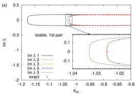
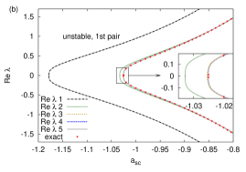
Figure 5: First pair of eigenvalues as a function of the scattering length, for an increasing number of coupled Gaussians and for the exact numerical calculation. (a) The two lowest eigenvalues of the stable ground state are purely imaginary. (b) The unstable excited state with a pair of purely real eigenvalues. Vanishing real or imaginary parts are not shown. The insets illustrate the rapid convergence of the variationally computed eigenvalues to the exact solutions of the Bogoliubov equations.

Similar to the calculation of the mean field energy and chemical potential, the pair of eigenvalues merges and vanishes at a tangent bifurcation. As we include more Gaussian functions, the critical scattering length shifts to higher values and converges to the bifurcation of the exact numerical solution as was expected from the behavior of the energies. Fig. 5(a) shows the first pair of eigenvalues of the stable ground state. They are purely imaginary. Since this is true for all stability eigenvalues of the ground state (see below), the branch of the ground state is stable. Fig. 5(b) shows the first eigenvalue pair of the excited state. These eigenvalues are purely real, and thus the excited state is unstable. The tangent bifurcation is clearly exhibited for both states, as each pair of eigenvalues $\pm\lambda$ merges at zero and vanishes at the critical scattering length.

It is important to note that similar to the convergence properties of the mean field energy and the chemical potential, very few coupled Gaussians are already sufficient to achieve excellent results for the lowest stability eigenvalues. Results obtained with $N\geq 3$ coupled Gaussians can not be distinguished in Fig. 5 from the numerically exact values.

II.2.2 Additional pairs of stability eigenvalues

In contrast to the calculation with a single Gaussian, which can provide only one pair of eigenvalues, additional eigenvalues are accessible when using coupled Gaussian wave functions. We compare them with the exact stability eigenvalues in Fig. 6.

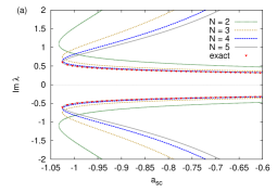
Figure 6: (a) Second pair of eigenvalues as a function of the scattering length, for varying number of coupled Gaussians and for the exact numerical calculation for the stable ground state and the unstable excited state. Numerically exact eigenvalues (triangles) are only available for the stable ground state. All eigenvalues are purely imaginary, vanishing real parts are not shown. (b) Same as (a) but for the third pair of eigenvalues.

The additional eigenvalues are increasingly difficult to obtain in the numerically exact computation. In the following, we refer to the eigenvalues with the second lowest absolute value simply as “second (pair of)” eigenvalues, etc. Numerically exact data is available for the lowest three pairs of eigenvalues of the stable ground state, and therefore here we compare the variational solution only with the lowest three eigenvalues of the stable solution.

Figure 6(a) shows the second pair of eigenvalues for the stable ground state and the unstable excited state. The second pairs of eigenvalues are all purely imaginary, and converge with increasing number of coupled Gaussians to the numerically exact eigenvalues.

The third pair of eigenvalues presented in Fig. 6(b) is qualitatively similar to the second pair. For any number of coupled Gaussians, they are purely imaginary. Figs. 6(a) and (b) suggest that, as the number of the eigenvalue rises, the convergence progresses more slowly. However, using five Gaussians in Fig. 6(b) even the third pair of the variational eigenvalues shows no apparent deviation from the numerically exact result.

II.2.3 Variations of the ground state wave function

We investigated the stability of the stationary states by linearizing the dynamical equations in the vicinity of the fixed points. For the stable ground state there are only purely imaginary eigenvalues, for the unstable excited state we found one pair of real eigenvalues. Additionally to the analysis of the eigenvalues $\lambda_{i}$ of the Jacobian of the linearized dynamical equations, we can evaluate the respective eigenvectors, which provide the form of the wave function’s fluctuations.

We focus on variations of the Gaussian parameters corresponding to the eigenvector $i$ and calculate the first order power series of the wave function $\psi(r,t)$ at the fixed point (FP) paper1 ,

$$\delta\psi_{i}(r,t)=\sum_{k=1}^{N} \left(\mathrm{i}r^{2}\delta a_{i}^{k,\mathrm{Re}}-r^{2}\delta a_{i}^{k,\mathrm{Im}}+\mathrm{i}\delta\gamma_{i}^{k,\mathrm{Re}}-\delta\gamma_{i}^{k,\mathrm{Im}}\right)$$

$$\times g^{k}|^{\mathrm{FP}}(r)\,\mathrm{e}^{\lambda_{i}t}.$$ (17)

For a scattering length of $a_{\mathrm{sc}}=-0.8$, Fig. 7

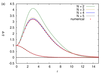
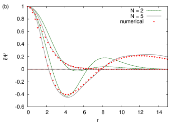
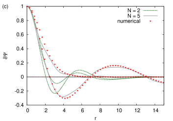
Figure 7: Deviations of the ground state wave function according to the eigenvectors of the (a) first, (b) second, and (c) third pair of eigenvalues $\pm\lambda$ of the stability analysis at scattering length $a_{\mathrm{sc}}=-0.8$.

shows the variation of the ground state wave function for the eigenvectors corresponding to the first (a), second (b) and third (c) pair of eigenvalues $\pm\lambda$ for the variational calculation, as well as for the numerically exact calculation.

In Fig. 7(a) the variation of the wave function $\delta\psi$ converges rapidly with increasing number of Gaussian functions to the numerical solution. For the second and third pair of eigenvalues in Fig. 7(b) and (c), the variation using five Gaussians is almost identical to the numerical variation. For the higher pairs of eigenvalues, the solution obviously converges slower. However, we note that it also becomes more and more difficult to obtain the exact solutions. The spatial extension of the fluctuations $\delta\psi$ exceeds the elongation of the wave function $\psi$ (cf. Figs. 2 and 3) by far and it becomes hard to achieve converged fluctuations. The differences between the numerical and the $N=5$ solution in Fig. 7(c) can already be explained by the quality of the numerical approach.

III Dipolar condensates

The stationary GPE for a dipolar BEC with a harmonic trap, the short-range s-wave scattering term and the long-range dipolar interaction reads

$$\bigg{[} -\Delta+\gamma_{x}^{2}x^{2}+\gamma_{y}^{2}y^{2}+\gamma_{z}^{2}z^{2}+8\pi N\frac{a}{a_{d}}\left|\psi(\bm{r})\right|^{2}$$

$$+N\int\mathrm{d}^{3}\bm{r}^{\prime}\frac{1-3\cos^{2}\theta}{\left|\bm{r}-\bm{r}^{\prime}\right|^{3}}\left|\psi(\bm{r}^{\prime})\right|^{2}\bigg{]}\psi(\bm{r})=\mu\psi(\bm{r})\;.$$ (18)

In Eq. (18) the “natural units” for this system introduced in gelbPatrick have been used, which are $\hbar$ for action, $m_{d}=2m$ for mass, $a_{d}={m_{d}\mu_{0}\mu^{2}}/(4\pi\hbar^{2})$ for length, $E_{d}={\hbar^{2}}/(m_{d}a_{d}^{2})$ for energy, and $\omega_{d}=E_{d}/\hbar$ for frequency. The angle between the external magnetic field in $z$-direction and the vector $\bm{r}-\bm{r}^{\prime}$ is denoted $\theta$, and $N$ is the particle number. As in gelbPatrick we scale ${\bm{r}}=N\tilde{\bm{r}}$, $\psi=N^{-\nicefrac{{3}}{{2}}}\tilde{\psi}$, insert the newly defined quantities in Eq. (18), redefine $\tilde{\gamma}_{i}=N^{2}\gamma_{i}$, $\tilde{\mu}=N^{2}\mu$, and afterwards omit the tilde once again. With the replacement $\mu\to\mathrm{i}(\mathrm{d}/\mathrm{d}t)$ we finally obtain the time-dependent GPE for a dipolar BEC in particle number scaled dimensionless units,

$$\bigg{[} -\Delta+\gamma_{x}^{2}x^{2}+\gamma_{y}^{2}y^{2}+\gamma_{z}^{2}z^{2}+8\pi a_{\mathrm{sc}}\left|\psi(\bm{r})\right|^{2}$$

$$+\int\mathrm{d}^{3}\bm{r}^{\prime}\frac{1-3\cos^{2}\theta}{\left|\bm{r}-\bm{r}^{\prime}\right|^{3}}\left|\psi(\bm{r}^{\prime})\right|^{2}\bigg{]}\psi(\bm{r})=\mathrm{i}\frac{\mathrm{d}}{\mathrm{d}t}\psi(\bm{r})\;,$$ (19)

with the trap frequencies $\gamma_{x,y,z}=N^{2}\omega_{x,y,z}/(2\omega_{d})$ and the s-wave scattering length $a_{\mathrm{sc}}=a/a_{d}$. For dipolar condensates it is possible to solve the GPE fully numerically on a two- or three-dimensional lattice Lahaye2009 ; Ronen06a . Ronen et al. Ronen and Dutta et al. duttadelle have shown that in certain regions of the parameter space dipolar condensates assume a non-Gaussian, biconcave, “blood-cell-like” shape. In this paper we want to apply the variational method with coupled Gaussian functions introduced in the preceding paper paper1 . We will show that the variational technique is a full-fledged alternative to the numerical simulations on grids, and additionally uncovers unstable stationary solutions not accessible in previous full-numerical evaluations.

The frequency and symmetry of the magnetic trap strongly influences the physical behavior of dipolar Bose-Einstein condensates. In the following we will analyze one distinct trap symmetry in detail, where the condensate has a blood-cell-shaped form. The ansatz with coupled Gaussians has proved to be capable to modify the simple Gaussian form of the wave function for monopolar condensates (see Sec. II.1). The biconcave shape, however, where the maximum density is no longer located at the origin is even a stronger challenge for the variational approach. We investigate the dipolar condensate for an axially symmetric trap with trap frequencies

$$\gamma_{x}=\gamma_{y}\equiv\gamma_{\varrho}=3600,\;\gamma_{z}=25200,$$

which is equivalent to the frequency ratio and mean

$$\lambda=\frac{\gamma_{z}}{\gamma_{\varrho}}=7,\;\bar{\gamma}=\sqrt[3]{\gamma_{\varrho}^{2}\gamma_{z}}=6887,$$

and corresponds to a value of $D=\sqrt{\gamma_{\varrho}}/2=30$ in Ronen . The trapping frequency in the $z$-direction parallel to the orientation of the dipoles is seven times larger than in the plane perpendicular to that direction, and for some parameters $a_{\mathrm{sc}}$ the ground state of the condensate has a biconcave, blood-cell-shaped form Ronen . In contrast to monopolar condensates where the inclusion of additional Gaussian functions provides an improved numerical accuracy of the results, dipolar condensates offer a wealth of new phenomena with increasing number of coupled Gaussian functions as will be shown below.

III.1 Variational calculations with one and two Gaussian functions

As ansatz for the variational calculations we use the wave function

$$\psi(\bm{r},t)=\sum_{k=1}^{N}\mathrm{e}^{\mathrm{i}\left(a_{x}^{k}x^{2}+a_{y}^{k}y^{2}+a_{z}^{k}z^{2}+\gamma^{k}\right)}\equiv\sum_{k=1}^{N}g^{k}\;,$$ (20)

where $N$ is the number of coupled Gaussians. For an axisymmetric trap the stationary solutions are also symmetric, i.e., $a_{x}^{k}=a_{y}^{k}\equiv a_{\varrho}^{k}$. Nevertheless, all stability properties have been computed with the fully three-dimensional ansatz. The case of a single Gaussian function ($N=1$) has been discussed in gelbPatrick . In this section we demonstrate that results especially for the mean field energy and chemical potential are already substantially improved with the use of only $N=2$ coupled Gaussians. Results of variational calculations with a single Gaussian function and numerical simulations on grids are employed for comparison and discussion.

III.1.1 Stationary solutions

Using the variational ansatz (20) stationary solutions of the Gross-Pitaevskii equation for dipolar BEC are obtained by a numerical root search for the fixed points of the dynamical equations for the variational parameters as described in detail in the preceding paper paper1 .

Figure 8 presents in (a) the mean field energy and in (b) the chemical potential for the two stationary solutions obtained with a single Gaussian function and with two coupled Gaussians.

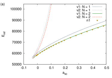
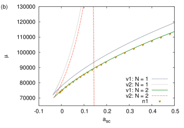
Figure 8: (a) Mean field energy and (b) chemical potential as a function of the scattering length, variational solution (v) using two Gaussians compared with an exact full-numerical lattice calculation (n1). For two Gaussians $(N=2)$, the ground state (v1) and the excited state (v2) emerge in a tangent bifurcation at $a_{\mathrm{sc}}=-0.034202$. The unstable branch of the chemical potential in (b) has a maximum at $\mu_{\max}\approx 170000$ (not shown) and then vanishes as a nearly vertical line at $a_{\mathrm{sc}}=1/6$.

For the ground state results of a numerical lattice calculation are also marked in Fig. 8. The numerical simulation was performed on a lattice with a grid size of $128\times 512$ points using fast-Fourier techniques and imaginary time evolution of an initial wave function.

The variational calculations with one Gaussian ($N=1$) show the following behavior. For scattering lengths below $a_{\mathrm{sc}}^{\mathrm{cr,var}}=-0.0378917$ there is no stable condensate. Similar as in monopolar condensates two solutions are born at the critical scattering length in a tangent bifurcation, the stable ground state (v1) and an unstable excited state (v2). For a detailed stability analysis see Sec. III.1.2 below. The unstable branch vanishes at scattering length $a_{\mathrm{sc}}=1/6$.

The variational ansatz with $N=1$ is limited to the Gaussian shape of the wave function with two width parameters $a_{\varrho}$ and $a_{z}$, and thus the values obtained for the mean field energy and chemical potential are not very accurate. However, the results are substantially improved when using a variational ansatz with two coupled Gaussians. This can be seen in Fig. 8 especially for the ground state when comparing the $N=2$ variational computation with the lattice computation (n1) marked by the triangles in Fig. 8.

In the full-numerical grid calculations only the ground state can be obtained. Starting with positive scattering lengths and decreasing $a_{\mathrm{sc}}$, the numerical grid calculations provide a ground state down to a critical point $a_{\mathrm{sc}}^{\mathrm{cr,num}}=-0.008$. Note that the ground state of the solution using two coupled Gaussian wave functions is nearly indistinguishable from the numerical lattice calculation in Figs. 8(a) and (b). An important advantage of the variational method is that it can provide both stable and unstable states. As will be shown below, the stability properties of the variational solutions can clarify the mechanism of how the condensate turns unstable.

Regarding the wave functions, one single Gaussian can evidently not adequately represent a blood-cell-shaped condensate. Two Gaussians not only significantly increase the accuracy of the mean field energy, but also greatly improve the form of the wave function. Even the biconcave shape of the dipolar condensate is qualitatively visible in the variational solution with two-Gaussians, however, the result is not fully converged. Exact wave functions will be compared in Sec. III.2 with variational results obtained with more than two coupled Gaussians.

III.1.2 Stability analysis

To perform a stability analysis with numerical lattice calculations the Bogoliubov-de Gennes equations have to be solved PitaevskiiBlackBook ; Ronen06a . Here we restrict our discussion to the stability analysis of the variational solutions, which is instructive considering nonlinear dynamics and bifurcation theory.

We follow the procedure outlined in paper1 and start with the stationary solutions of the GPE calculated using one and two Gaussians. These solutions are fixed points of the dynamical equations for the Gaussian parameters. We then linearize these dynamical equations in the vicinity of the fixed point and calculate the eigenvalues of the Jacobian (see paper1 ).

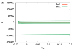
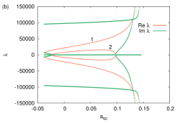
Figure 9: Eigenvalues of the Jacobian for the variational solution with one Gaussian as a function of the scattering length $a_{\mathrm{sc}}$. (a) The ground state is stable, all eigenvalues are purely imaginary, (b) the excited state is unstable since there are real parts of eigenvalues, emerging in a tangent bifurcation at $a_{\mathrm{sc}}^{\mathrm{cr}}=-0.0378917$. Eigenvalues which do not reach $\lambda=0$ at $a_{\mathrm{sc}}^{\mathrm{cr}}$ match with the corresponding eigenvalues of the stable and unstable state, respectively.

The eigenvalues of the ground state obtained with one Gaussian wave function in Fig. 9(a) are purely imaginary. Therefore this state is stable. If we perturb the variational parameters of the fixed point solution, the quasi-periodic motion is confined to the vicinity of the fixed point.

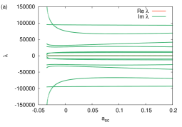
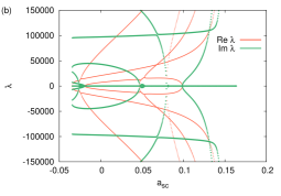
Figure 10: Same as Fig. 9 but for the variational calculation with two coupled Gaussians, (a) the stable ground state and (b) the unstable excited state. Additional eigenvalues are revealed. The tangent bifurcation is shifted to $a_{\mathrm{sc}}^{\mathrm{cr}}=-0.034202$. Eigenvalues which do not reach $\lambda=0$ at $a_{\mathrm{sc}}^{\mathrm{cr}}$ match with the corresponding eigenvalues of the stable and unstable state, respectively.

Figure 9(b) shows the characteristic eigenvalues of the unstable excited state. Contrary to the stable state, there are eigenvalues with non-vanishing real parts $\mathrm{Re}\,\lambda$. Perturbations in the direction of the corresponding eigenvector lead to an exponential growth of the perturbation. Therefore this state is unstable. Both branches exist for scattering lengths down to $a_{\mathrm{sc}}^{\mathrm{cr}}=-0.0378917$, where they merge in a tangent bifurcation (see Fig. 8). The tangent bifurcation is apparent in the eigenvalues in Figs. 9(a) and (b).

Some eigenvalues of the Jacobian using a wave function of two coupled Gaussians in Fig. 10 qualitatively agree with the one-Gaussian calculation. There is one stable ground state with purely imaginary eigenvalues in Fig. 10(a), and one unstable excited state in Fig. 10(b). However, the two-Gaussian calculation yields additional eigenvalues which are not available within the limited parameter space of the simple one-Gaussian calculation.

The unstable branches of both calculations in Figs. 9(b) and 10(b), exhibit that for the given parameters of the trap in dipolar condensates, the stability scenario is quite more complex than for monopolar condensates. As we can see, there is not only one single pair of imaginary eigenvalues of the stable solution approaching zero and merging with one pair of real unstable eigenvalues (denoted 1 in Fig. 9(b)) from the excited state. For monopolar condensates this real pair of eigenvalues of the unstable solution remains the only one for increasing scattering lengths (see Sec. II.2). By contrast, here, a second pair of eigenvalues (denoted 2 in Fig. 9(b)) indicating instability additionally forms as we follow the excited state from the bifurcation point to positive scattering lengths. The eigenvectors that correspond to this pair of real eigenvalues also show an interesting behavior: The stability analysis is performed in three dimensions although the solutions of the GPE are axisymmetric. Therefore in the linearization around the fixed point, perturbations in $x$ and $y$ direction are calculated independently. The eigenvectors corresponding to the additional unstable eigenvalues are not symmetrical in $x$ and $y$, and thus break the axial symmetry of the fixed point solution.

The unstable branch of the calculation with two Gaussians already shows multiple pairs of unstable real eigenvalues. This suggests that the dynamics of dipolar condensates in this parameter region is very complex and can be described better by including even more coupled Gaussians in the variational approach. Indeed, the further increase of the number of variational parameters reveals new physical properties and phenomena also of the ground state of the biconcave dipolar condensate.

III.2 Converged variational calculations with up to six coupled Gaussian functions

Since the inclusion of two Gaussians already substantially improves the mean field energy, the coupling of more functions only results in a minor correction in the value of the mean field energy, which would not be apparent in, e.g., Fig. 8. We therefore present in Fig. 11(a) the convergence of the mean field energy at one selected scattering length, viz. $a_{\mathrm{sc}}=0$, for $N=2$ to $N=6$ coupled functions.

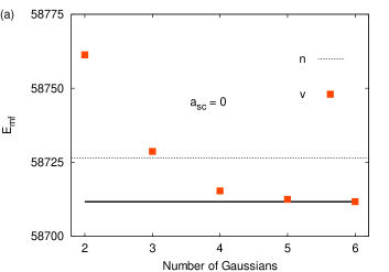
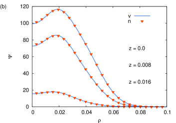
Figure 11: (a) Convergence of the mean field energy (to the solid line) with increasing number of coupled Gaussian wave functions for $a_{\mathrm{sc}}=0$. The mean field energy for four coupled functions lies already energetically lower than the numerical value of the lattice computation (dashed line). (b) The converged wave function $\psi$ as a function of the transverse coordinate $\varrho$ at different $z$ coordinates. The variational solution and the numerical lattice solution are denoted v and n, respectively.

For other scattering lengths the convergence behavior is similar. This example shows that as few as four coupled Gaussian functions result in a mean field energy which lies below the numerical solution of the lattice calculation (dashed line). For five and six Gaussians, the variational solution converges to a distinct value (solid line). Note that the simplest variational solution with one Gaussian function is not included in the figure because the mean field energy of $E_{\mathrm{mf}}=60361$ lies far outside the vertical energy scale.

In Fig. 11(b) for the same scattering length ($a_{\mathrm{sc}}=0$) the converged wave function is shown at different $z$ coordinates. The wave function of the variational calculation is practically identical to the wave function of the numerical lattice calculation. Both wave functions show the characteristic biconcave shape of the condensate.

In this section, we discuss properties of the solutions obtained with five and six coupled Gaussians, which are qualitatively identical and quantitatively indistinguishable in the figures presented. Therefore we will omit the detailed label and refer to the converged variational solution simply as “variational solution” (v). While the use of one and two coupled Gaussians in Sec. III.1 results in two branches, one stable, one unstable, emerging in a tangent bifurcation, this bifurcation scenario has to be revised with the converged variational solution.

Figure 12(a) shows an overview of the mean field energy for the variational solution. There are two important intervals of the scattering length $a_{\mathrm{sc}}$, showing different characteristics of the variational solution with coupled Gaussian functions. These intervals of the scattering length are marked in Fig. 12(a).

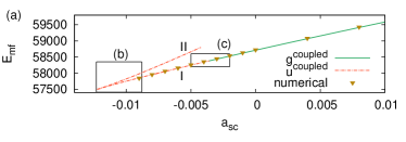
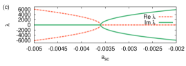
Figure 12: (a) Overview of the mean field energy for the bifurcation scenario revealed in the variational calculation. For comparison some values of the numerical lattice solution for the ground state are presented (see text for more details). The stability eigenvalues in the regions around the critical scattering lengths $a^{\mathrm{cr,t}}_{\mathrm{sc}}=-0.01224$ and $a^{\mathrm{cr,p}}_{\mathrm{sc}}=-0.00359$ marked by the black frames in (a) are shown in (b) and (c), respectively. In (b) I and II denote the two merging branches. Only the eigenvalues involved in the bifurcation are shown (for analysis and interpretation see text). Eigenvalues of the Jacobian as a function of the scattering length in (c) indicate the stability change of the ground state in a pitchfork bifurcation. The unstable state for $a_{\mathrm{sc}}<a_{\mathrm{sc}}^{\mathrm{cr,p}}=-0.00359$ turns into the stable ground state for $a_{\mathrm{sc}}>a_{\mathrm{sc}}^{\mathrm{cr,p}}$ in a pitchfork bifurcation. Subfigure (c) only shows the lowest eigenvalues, those involved in the stability change.

The different line styles in Fig. 12(a) indicate the stability of the solutions anticipating the results of the stability analysis. The numerical solution via lattice calculation and imaginary time evolution obtains only the ground state. Note that the numerical simulation was carried out on a two-dimensional axisymmetric grid, and thus the imaginary time evolution can provide unstable ground states if the instability is rotational, i.e., resulting in an angular collapse of the condensate WilsonPRA80 .

The variational solution is able to obtain both, the stable ground state and stationary excited states. There are variational results down to a critical point $a_{\mathrm{cr}}^{\rm t}=-0.01224$. To analyze the stability of the solution, we present in Fig. 12(b) a stability analysis of the linearized dynamical equations in the interval $-0.0123<a_{\mathrm{sc}}<-0.0088$ of the scattering length [frame marked (b) in Fig. 12(a)].

Figure 12(b) shows at the center the typical scenario of eigenvalues of two branches merging in a tangent bifurcation at $a_{\mathrm{cr}}^{\rm t}=-0.01224$. A pair of purely imaginary eigenvalues of the branch denoted I merges at a critical point with a pair of real eigenvalues of branch II. Respective vanishing real or imaginary parts are not shown.

In addition to this tangent bifurcation there is a direction in Gaussian parameter space, in which both branches show unstable, purely real eigenvalues (see Fig. 12(b) top and bottom). Therefore both branches involved in the tangent bifurcation are born unstable.

The previous scenario which resulted from the calculation with one or two coupled Gaussians in Sec. III.1 must now be revised. In the converged variational ansatz, the tangent bifurcation is on top of an unstable direction. The important conclusion is that there is no stable condensate in this region of the scattering length.

Where does the variational condensate turn stable? To pursue this question we increase the scattering length to $a_{\mathrm{sc}}\approx-0.00359$ [frame marked (c) in Fig. 12(a)]. The corresponding stability analysis shows a stability change for the lowest eigenvalues of the ground state, which are plotted in Fig. 12(c).

For scattering lengths $a_{\mathrm{sc}}<a_{\mathrm{sc}}^{\mathrm{cr,p}}=-0.00359$ the branch is unstable, indicated by the pair of real eigenvalues in Fig. 12(c). At this bifurcation point the real eigenvalues vanish and for $a_{\mathrm{sc}}>a_{\mathrm{sc}}^{\mathrm{cr,p}}=-0.00359$ a stable ground state forms, indicated by a pair of imaginary eigenvalues. Figure 12(c) shows only the respective lowest pair of eigenvalues which is involved in the stability change, all other eigenvalues are purely imaginary, and are omitted for the sake of clarity of the figure.

The stability change of the ground state in Fig. 12(a) takes place in a pitchfork bifurcation. From left to right, one unstable branch turns stable in the bifurcation.

In general, three branches are involved in a pitchfork bifurcation OttChaos . If the ground state of the dipolar condensate changes stability in a pitchfork bifurcation, two stable states should appear as stationary states in the variational calculation for the dipolar BEC as well. However, for the following reasons we are probably unable to observe these additional stable states directly. There are $4N$ complex Gaussian variational parameters, i.e. 48 real parameters for six coupled functions. The pitchfork bifurcation and the stability change take place in one direction characterized by the eigenvectors of the eigenvalues shown in Fig. 12(c). Since an increasing number of variational parameters leads to a more and more complex parameter space with increasingly complex interactions between the degrees of freedom, it is well possible that the two stable states are limited to an extremely tiny vicinity of the bifurcation point.

For scattering lengths greater than the bifurcation, the ground state is stable. At the bifurcation the system also changes from regular dynamics to chaotic dynamics, where for scattering lengths below the bifurcation point both additional stable branches may undergo several bifurcations themselves, immediately turning them unstable. Therefore it is not possible to obtain the stable branches directly via search for fixed points of the dynamical equations.

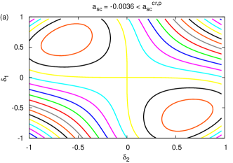
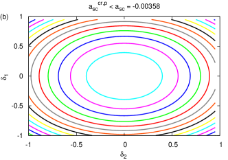
Figure 13: Contour plot of the mean field energy (a) for $a_{\mathrm{sc}}=-0.0036$ closely below, and (b) for $a_{\mathrm{sc}}=-0.00358$ closely above the pitchfork bifurcation. The eigenvectors corresponding to the eigenvalues in Fig. 12(c) linearize the vicinity of the fixed point ($\delta_{1}$ and $\delta_{2}$, arbitrary units).

However, it is possible to catch a glimpse of those branches, if we consider the linearized surroundings of the stability changing state very close to the bifurcation.

The eigenvectors corresponding to the lowest eigenvalues (that show the stability change) linearize the vicinity of the stationary state $(\delta_{1},\delta_{2})$. Figure 13 shows the contour plot of the mean field energy of this linearization in arbitrary units for two scattering lengths (a) very close below and (b) very close above the bifurcation. Above the bifurcation Fig. 13(b) shows one elliptic stable state, the stable ground state. Below the bifurcation, Fig. 13(a) shows the unstable fixed point at the center. Besides the unstable hyperbolic fixed point, there are two stable elliptic points at ($\pm 0.5,\mp 0.5$) in this vicinity linearized by the eigenvectors. Nevertheless, Fig. 13 is limited to the two-dimensional plane spanned by two eigenvectors. If all directions of the eigenvectors of all eigenvalues are considered, those two states are only stable in a very small interval $a_{\mathrm{sc}}^{\mathrm{cr,p}}-\epsilon<a_{\mathrm{sc}}<a_{\mathrm{sc}}^{\mathrm{cr,p}}$ below the bifurcation point, which makes them numerically impossible to find. Due to the numerically small value of $\epsilon$, however, the classification of the condensate as unstable for scattering lengths $a_{\mathrm{sc}}<a^{\mathrm{p}}_{\mathrm{cr}}=-0.0359$ remains true in physical terms.

If we further investigate the two eigenvectors that correspond to the pair of eigenvalues in which the stability change occurs, we see, that the axial symmetry is no longer present. For the present trap symmetry and frequencies $(\gamma_{x}=\gamma_{y}=3600$ and $\gamma_{z}=25200)$ and the ansatz

$$\psi(\varrho,z)=\sum_{k=1}^{N}\mathrm{e}^{\mathrm{i}\left(a_{\varrho}^{k}\varrho^{2}+a_{z}^{k}z^{2}+\gamma^{k}\right)}\;,$$ (21)

all fixed points had been axisymmetric. The stability analysis, however, is done without any assumptions considering symmetry, allowing variations in both, $\delta a^{k}_{x}$ and $\delta a^{k}_{y}$ separately. Therefore, oscillations in directions which break the axial symmetry are allowed.

The characteristic eigenvectors can be considered as deviations of the wave function $\delta\psi$ (see paper1 ). If the eigenvector is no longer axially symmetric, i.e., $\delta a_{x}^{k}=-\delta a_{y}^{k}$ for all $k$, the perturbation leads to an asymmetric oscillation or collapse of the condensate. Indeed, we find this kind of eigenvectors for the lowest eigenvalues of the Jacobian for the variational solution of the ground state in Fig. 12(c). This behavior of the eigenvectors of the Jacobian is an indication of the so called “angular collapse of dipolar BEC” associated with the biconcave shape of the condensate WilsonPRA80 .

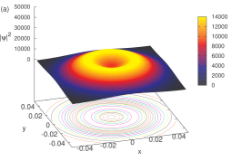
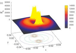
Figure 14: Time evolution of the perturbed particle density $|\psi|^{2}$ of the unstable stationary solution as a function of $x$ and $y$ for $z=0$ for (a) $t=0.0001$, (b) $t=0.005$, and (c) $t=0.006$.

This angular collapse can be observed in a time evolution of the condensate. We prepare the stationary wave function for a scattering length closely below the bifurcation, and add a deviation

$$\psi(\bm{z})=\psi(\bm{z}^{\mathrm{FP}})+\delta\psi(\delta\bm{z}_{i})$$ (22)

in the direction of the eigenvector $i$ whose corresponding eigenvalue is involved in the stability change. Figure 14 shows a time evolution of the particle density $|\psi|^{2}$ obtained by numerical integration of the dynamical equations. The time evolution of the unstable excited state clearly reveals an angular collapse of the condensate, the particle density concentrates on two non-axially symmetric regions as shown in Fig. 14. The Gaussian ansatz (20) implies a collapse of the condensate with parity with respect to the $x$ and $y$ axis, but it may be possible in future work to modify the Gaussian functions to include any form of collapse without symmetry restrictions. A modified ansatz may even allow for an angular collapse of the condensate with three density peaks as reported by Wilson et al. WilsonPRA80 .

IV Conclusion

We have applied the method of coupled Gaussian wave packets to Bose-Einstein condensates with two different types of long-range interaction, viz. an attractive gravity-like $1/r$ interaction and a dipole-dipole interaction. The mean field energy and chemical potential have been obtained as fixed points of dynamical equations for the set of variational parameters. As an alternative to solving the Bogoliubov equations the stability properties of the condensates have been determined by applying methods of nonlinear dynamics to the linearized equations of motion.

For monopolar condensates we have shown that the additional variational parameters of the coupled Gaussian ansatz greatly improve the accuracy of the variational solution in comparison to the established single Gaussian ansatz. With three coupled Gaussian functions in the trial wave function, the numerical mean field energy is already reproduced with an accuracy of more than four digits. The solution with five Gaussians proves to be fully converged to the solution of the direct numerical integration of the GPE. Furthermore, the stability properties and the bifurcation of the numerical solution are excellently reproduced by the coupled Gaussian ansatz. The variational method also provides easy access to higher stability eigenvalues, which numerically are hard to obtain. For monopolar condensates, the method of coupled Gaussian functions is an excellent and fully valid alternative to the direct numerical integration of the GPE.

For dipolar condensates we have described the new phenomena revealed by variational solutions with an increasing number of coupled Gaussians. The variational ansatz with multiple coupled Gaussian functions turns out to be a full-fledged alternative to numerical lattice calculations for condensates with dipolar interaction. With the use of as little as five to six Gaussian functions, the variational solution can be considered to be fully converged. In contrast to lattice calculations via imaginary time evolution, the variational ansatz also obtains excited states. Thus the method of coupled Gaussian functions gives access to yet unexplored regions of the space of solutions of the GPE, and we have been able to clarify the theoretical nature of the collapse mechanism: The ground state of the condensate turns unstable in a pitchfork bifurcation before it finally vanishes in a tangent bifurcation. The stability analysis indicates a further feature of the collapse mechanism: The condensate breaks the cylindrical symmetry on the verge of collapse, indicating an angular decay of the condensate.

The convergence of the variational method with Gaussians has proved to be very fast even close to the critical scattering length, at which the collapse of the condensate sets in. In future work it will be interesting to monitor the convergence of the ansatz in the Thomas-Fermi regime, where exact polynomial solutions of the wave functions are found ODellPRL84 ; ODel04 ; Ebe05 . It will also be desirable to investigate in more detail how the numerical stability analysis via the Bogoliubov-de Gennes equations is related to the variational stability analysis. Furthermore it will be possible to investigate real time dynamics of the decay of dipolar BEC and angular rotons with a modified coupled Gaussian ansatz. The coupled Gaussian ansatz proved to be a fast and accurate alternative to full-numerical calculations. There are several interesting systems where this method can be applied in future work, e.g., monopolar BEC with vortices or stacks of dipolar condensates.

References

- (1) S. Rau, J. Main, and G. Wunner, preceding paper, submitted
- (2) D. O’Dell, S. Giovanazzi, G. Kurizki, and V. M. Akulin, Phys. Rev. Lett. 84, 5687 (2000)
- (3) R. Ruffini and S. Bonazzola, Phys. Rev. 187, 1767 (1969)
- (4) I. Papadopoulos, P. Wagner, G. Wunner, and J. Main, Phys. Rev. A 76, 053604 (2007)
- (5) H. Cartarius, J. Main, and G. Wunner, Phys. Rev. A 77, 013618 (2008)
- (6) H. Cartarius, T. Fabčič, J. Main, and G. Wunner, Phys. Rev. A 78, 013615 (2008)
- (7) A. Griesmaier, J. Werner, S. Hensler, J. Stuhler, and T. Pfau, Phys. Rev. Lett. 94, 160401 (2005)
- (8) J. Stuhler, A. Griesmaier, T. Koch, M. Fattori, T. Pfau, S. Giovanazzi, P. Pedri, and L. Santos, Phys. Rev. Lett. 95, 150406 (2005)
- (9) Q. Beaufils, R. Chicireanu, T. Zanon, B. Laburthe-Tolra, E. Maréchal, L. Vernac, J.-C. Keller, and O. Gorceix, Phys. Rev. A 77, 061601(R) (2008)
- (10) T. Koch, T. Lahaye, J. Metz, B. Fröhlich, A. Griesmaier, and T. Pfau, Nature Physics 4, 218 (2008)
- (11) S. Ronen, D. C. E. Bortolotti, and J. L. Bohn, Phys. Rev. Lett. 98, 030406 (2007)
- (12) S. Ronen, D. C. E. Bortolotti, and J. L. Bohn, Phys. Rev. A 74, 013623 (2006)
- (13) R. M. Wilson, S. Ronen, and J. L. Bohn, Phys. Rev. A 80, 023614 (2009)
- (14) P. Köberle, H. Cartarius, T. Fabčič, J. Main, and G. Wunner, New Journal of Physics 11, 023017 (2009)
- (15) T. Lahaye, C. Menotti, L. Santos, M. Lewenstein, and T. Pfau, Rep. Prog. Phys. 72, 126401 (2009)
- (16) S. Rau, J. Main, P. Köberle, and G. Wunner, Phys. Rev. A 81, 031605(R) (2010)
- (17) C. Huepe, L. S. Tuckerman, S. Métens, and M. E. Brachet, Phys. Rev. A 68, 023609 (2003)
- (18) S. Giovanazzi, G. Kurizki, I. E. Mazets, and S. Stringari, Europhys. Lett. 56, 1 (2001)
- (19) O. Dutta and P. Meystre, Phys. Rev. A 75, 053604 (2007)
- (20) L. Pitaevskii and S. Stringari, Bose-Einstein Condensation (Oxford Science Publications, 2008)
- (21) E. Ott, Chaos in Dynamical Systems (Cambridge University Press, 1993) p. 44
- (22) D. H. J. O’Dell, S. Giovanazzi, and C. Eberlein, Phys. Rev. Lett. 92, 250401 (2004)
- (23) C. Eberlein, S. Giovanazzi, and D. H. J. O’Dell, Phys. Rev. A 71, 033618 (2005)