General Relativistic Ray-Tracing Method for Estimating the Energy and Momentum Deposition by Neutrino Pair Annihilation in Collapsars

Abstract

Bearing in mind the application to the collapsar models of gamma-ray bursts (GRBs), we develop a numerical scheme and code for estimating the deposition of energy and momentum due to the neutrino pair annihilation ($\nu+{\bar{\nu}}\rightarrow e^{-}+e^{+}$) in the vicinity of accretion tori around a Kerr black hole. Our code is designed to solve the general relativistic neutrino transfer by a ray-tracing method. To solve the collisional Boltzmann equation in curved spacetime, we numerically integrate the so-called rendering equation along the null geodesics. We employ the Fehlberg(4,5) adaptive integrator in the Runge-Kutta method to perform the numerical integration accurately. For the neutrino opacity, the charged-current $\beta$-processes are taken into account, which are dominant in the vicinity of the accretion tori. The numerical accuracy of the developed code is certificated by several tests, in which we show comparisons with the corresponding analytic solutions. In order to solve the energy dependent ray-tracing transport, we propose that an adaptive-mesh-refinement approach, which we take for the two radiation angles $(\theta,\phi)$ and the neutrino energy, is useful to reduce the computational cost significantly. Based on the hydrodynamical data in our collapsar simulation, we estimate the annihilation rates in a post-processing manner. Increasing the Kerr parameter from 0 to 1, it is found that the general relativistic effect can increase the local energy deposition rate by about one order of magnitude, and the net energy deposition rate by several tens of percents. After the accretion disk settles into a stationary state (typically later than $\sim 9$ s from the onset of gravitational collapse), we point out that the neutrino-heating timescale in the vicinity of the polar funnel region can be shorter than the dynamical timescale. Our results suggest the neutrino pair annihilation has a potential importance equal to the conventional magnetohydrodynamic mechanism for igniting the GRB fireballs.

1 Introduction

Gamma-ray bursts (GRBs) have long attracted the attention of astrophysicists since their accidental discovery in 1970s. Regarding the long-duration GRBs, there have been accumulating observations identifying a massive stellar collapse as their origin (e.g., Woosley & Bloom (2006) for a review). The duration of the long bursts may correspond to the accretion of debris falling into the central black hole (BH) (Piro et al., 1998). It suggests the observational consequence of the BH formation likewise the supernova of neutron star formation. For their central engines, the so-called collapsar has received quite some interest for more than decade (Woosley, 1993; Paczynski, 1998; MacFadyen & Woosley, 1999).

In the collapsar scenario, the central cores with significant angular momentum collapse into a black hole. Neutrinos emitted from the accretion disk heat matter in the polar funnel region to launch the GRB outflows. Paczynski (1990); Meszaros & Rees (1992) pioneerlingly proposed that the energy deposition proceeds predominantly via neutrino and antineutrino annihilation into electron and positron (e.g., $\nu+{\bar{\nu}}\rightarrow e^{-}+e^{+}$, hereafter “neutrino pair annihilation”). In addition, it is suggested that the strong magnetic fields in the cores of order of $10^{15}\,\,\mathrm{G}$ play also an active role both for driving the magneto-driven jets and for extracting a significant amount of energy from the central engine (e.g., Blandford & Znajek (1977); Thompson et al. (2004); Uzdensky & MacFadyen (2007) and see references therein).

However, it is still controversial whether the generation of the relativistic outflows proceeds predominantly via magnetohydrodynamic (MHD) or neutrino-heating processes. So far, much attention has been paid to the MHD processes (e.g., Proga (2003); Mizuno et al. (2004); Lyutikov (2006); Fujimoto et al. (2006); Nagataki et al. (2007); McKinney & Narayan (2007); Komissarov & Barkov (2007); Barkov & Komissarov (2008); Nagataki (2009); Harikae et al. (2009)). A general outcome of these extensive MHD simulations is that the magneto-driven shock waves can blow up massive stars along the rotational axis. Those primary jet-like explosions are firstly at most mildly relativistic due to too much baryons in the central core (e.g., Takiwaki et al. (2009)), however could be relativistic as they propagate further out (Nagataki, 2009). In such a collapsar environment, explosive nucleosynthesis (e.g., Fujimoto et al. (2006); Nagataki et al. (2007), neutrino and gravitational-wave signals (e.g., Kawagoe et al. (2009); Hiramatsu et al. (2005)), have been also extensively studied.

In contrast to such blossoms in the MHD studies, there have been only a few studies pursuing the possibility of generating jets by the energy deposition via neutrino pair annihilation. This is mainly because the neutrino emission from the accretion disk generally becomes highly aspherical, thus demanding us to solve a multidimensional neutrino transfer problem (e.g., Tubbs (1978); Janka & Hillebrandt (1989)). This is still computationally very expensive, which is also the case for the neutrino-driven supernova simulations (see references in Janka et al. (2007)). For the first time in the collapsar simulations, MacFadyen & Woosley (1999) pointed out the importance of the energy deposition via neutrino pair annihilation, however the energy deposition rates to the polar funnel region were adjusted by hand to produce jets. To our best knowledge, the fast and collimated neutrino-heated outflows have not been realized so far in the numerical simulations without the artificial energy injection to the polar funnel regions (see, e.g., Aloy et al. (2000); Zhang et al. (2003); Mizuta & Aloy (2009) and references therein).

Thus far, there have been reported several methods aiming to implement the neutrino pair annihilation into the collapsar simulations. By estimating the fluxes and spectra of the neutrino emission from the accretion disk via the so-called neutrino leakage scheme, Ruffert et al. (1997); Ruffert & Janka (1998) proposed to estimate the heating rate by summing up the contributions of the neutrino and antineutrino radiation incident from all directions. Along this prescription, Nagataki et al. (2007) have estimated the neutrino heating rates, and included them to the hydrodynamical simulation. For reducing the computational time, they added one more assumption of the optically thinness of the accretion disk to the prescription by Ruffert & Janka (1998). Even with this potential overestimation of the heating rates, the neutrino-driven outflows were not observed in their simulations. More recently, Dessart et al. (2009) have developed a new scheme to estimate the energy deposition rate using the state-of-the-art, multi-angle neutrino-transport solver (Ott et al., 2008a). They discussed the possible formation of the neutrino-driven outflow in the postmerger phase of binary neutron-star coalescence. Relying on the neutrino leakage scheme, Harikae et al. (2010) have proposed a special relativistic ray-tracing method to estimate the annihilation rates. Using hydrodynamical data in their collapsar simulation, they pointed out that the neutrino-heated outflow might be formed in $\sim$ 10 seconds after the initial collapse of the progenitor star.

It should be noted that all of the above schemes neglect the general relativistic (GR) effects for simplicity, which have been reported to enhance the annihilation rates significantly near the accreting black holes (e.g., Jaroszynski (1993, 1996); Salmonson & Wilson (1999); Asano & Fukuyama (2001, 2000); Birkl et al. (2007)). Among the GR studies, the numerical method of Birkl et al. (2007) would be one of the most sophisticated one, in which a ray-tracing calculation is performed to follow the neutrino trajectories in a Kerr spacetime. The ray-tracing method has an advantage because it can straightforwardly capture important GR features such as the ray bending and redshift. In their scheme, the neutrino number flux emitted from the accretion disk (or from the neutrino spheres) is simply assumed to be conserved along the geodesics. In reality, the neutrino emission, absorption, and scattering should occur along the neutrino geodesics changing its neutrino distribution function simultaneously. Especially in the absence of the charged-current neutrino interactions, the annihilation rates in Birkl et al. (2007) could be overestimated. To improve these issues, one has to solve the general relativistic neutrino transport equation along each ray, which we are to investigate in this paper.

In this study, we present a numerical code and scheme for calculating the deposition of energy and momentum via neutrino pair annihilation in a Kerr spacetime, in which we solve the general relativistic radiative equation along the null geodesics. The charged-current $\beta$-processes are taken into account, which are dominant in the vicinity of the accretion tori (e.g., Dessart et al. (2009)). With these improvements, the newly developed code would provide a more realistic estimation of the annihilation rates than before. We check the numerical accuracy of the developed code by showing several comparison with analytic solutions, some of which we newly derive in this paper. Based on the results of our long-term collapsar simulation (Harikae et al., 2009), we run our new code to estimate the annihilation rate in a post-processing manner and discuss their implications on the dynamics of collapsars.

This paper is organized as follows. In Section 2, we summarize the formulation of the general relativistic ray-tracing method for the collisional Boltzmann equation. Section 3 is devoted to the numerical tests. In Section 4, we estimate the annihilation rates in a post-processing manner using hydrodynamical data in our collapsar simulation. We summarize our results and discuss their implications in Section 5.

2 Neutrino Pair Annihilation in General Relativity

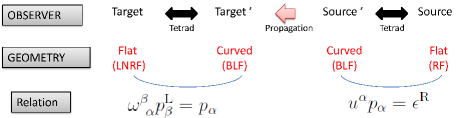
Figure 1: Schematic picture of relations of energy/momentum among three frames (LNRF, BLF, RF). Upper script R denotes the variables measured in RF, while upper script L denotes the variables measured in LNRF.

In this section, we summarize the formalism and our strategy to estimate the neutrino-pair-annihilation rates based on the general relativistic radiation transfer. In section 2.1, we summarize the method to solve the neutrino geodesics in a Kerr spacetime for the collisionless Boltzmann equation. Then in section 2.2, we move on to mention how to solve the collisional Boltzmann equation along the geodesics.

We assume that the gravitational field, which leads to ray bending and redshift, is given by the central Kerr BH of mass $M$ and angular momentum parameter $a\equiv J/M$ (where $J$ is the angular momentum of the BH, and $0\leq a/M\leq 1$), whose metric is given in the Boyer-Lindquist coordinates ($t,r,\theta,\phi$) by

$$ds^{2} = g_{\alpha\beta}dx^{\alpha}dx^{\beta},$$ (1)

$$= -\alpha^{2}dt^{2}+\gamma_{ij}(dx^{i}+\beta^{i}dt)(dx^{j}+\beta^{j}dt),$$

where the lapse function $\alpha$, the shift vector $\beta^{i}$ and the non-vanishing components of the spatial metric $\gamma_{ij}$ are given as

$$\alpha=\sqrt{\frac{\Sigma\Delta}{A}},~{}\beta^{\phi}=-\omega,~{}\gamma_{rr}=\frac{\Sigma}{\Delta},~{}\gamma_{\theta\theta}=\Sigma,~{}\gamma_{\phi\phi}=\frac{A\sin^{2}\theta}{\Sigma},$$ (2)

where $\Sigma=r^{2}+a^{2}\cos^{2}\theta$, $\Delta=r^{2}-2Mr+a^{2}$, $A=(r^{2}+a^{2})^{2}-a^{2}\Delta\sin^{2}\theta=\Sigma\Delta+2Mr(r^{2}+a^{2})$, and $\omega=2aMr/A$ (e.g., Misner et al. (1973)). Here we use $G=c=1$ unit and note that the Latin indices ($i,j$) have the domain of $(r,\theta,\phi)$. For later convenience, we also define the dimensionless angular momentum parameter of $a^{*}=a/M$.

For later convenience, we first introduce the following three frames, the Boyer-Lindquist frame (BLF) which is given by the center of mass system in curved space-time, the locally non-rotating frame (LNRF) which is given by the tetrad frame rotating with the central BH to make the dragging effects vanish (i.e., $e_{i}=0$ with $e_{\mu}$ being the basis of the vierbein), and the rest frame of fluid (RF) which is necessary to define quantities related to radiation such as emissivity and absorptivity. These three frames can be connected with each other by the tetrad and Lorentz transformations. In the following sections, the quantities measured in the LNRF and RF are denoted by the superscript “L” and “R”, respectively. Variables in the BLF are denoted without any superscripts. A schematic picture between these three frames are illustrated in Figure 1. What we finally need is the annihilation rates measured by the observer in the LNRF (left-end in the figure). The neutrino emissivity and absorptivity are naturally defined in the rest frame of fluid (RF), in which the radiation isotropy is maintained (right-end in the figure). The first step is to transform the variables in the RF to the ones in the BLF (from the right-end to left by one step) using the tetrad transformation (the “relation” shown in the figure with some formulae will be derived later in this section). The second step is to do the ray-tracing calculation from the source to the target in the global BLF (indicated by “Target^′ ” in the figure). Finally the annihilation rates in the LNRF is given by the tetrad transformation form the BLF to the LNRF. In the following, we explain these procedures more in detail.

The local annihilation rate in the LNRF (e.g., Goodman et al. (1987); Asano & Fukuyama (2000); Birkl et al. (2007)) is written as,

$$Q_{\mu}^{\rm L}(\mbox{\boldmath$r$}) = 2KG_{\rm F}^{2}\int d^{3}{\mbox{\boldmath$p$}}^{\rm L}_{\nu}d^{3}{\mbox{\boldmath$p$}}^{\rm L}_{\bar{\nu}}$$ (3)

$$\times(\epsilon^{\rm L}_{\nu}\epsilon^{\rm L}_{\bar{\nu}})({\mbox{\boldmath$p$}}^{\rm L}_{\nu}+{\mbox{\boldmath$p$}}^{\rm L}_{\bar{\nu}})_{\mu}f^{\rm L}_{\nu}(\mbox{\boldmath$p$}^{\rm L}_{\nu},\mbox{\boldmath$r$})f^{\rm L}_{\bar{\nu}}(\mbox{\boldmath$p$}^{\rm L}_{\bar{\nu}},\mbox{\boldmath$r$})$$

$$\times\left[1-\sin{\theta_{\nu}}\sin{\theta_{\bar{\nu}}}\cos{(\varphi_{\nu}-\varphi_{\bar{\nu}})}-\cos{\theta_{\nu}}\cos{\theta_{\bar{\nu}}}\right]^{2},$$

where $f^{\rm L}_{\nu}$ is the number density of neutrinos in the phase space within the solid angle of $d\Omega_{\nu}=\sin{\theta_{\nu}}d\theta_{\nu}d\varphi_{\nu}$ in the momentum space, $\mbox{\boldmath$p$}^{\rm L}_{\nu}$ and $\epsilon^{\rm L}_{\nu}$ is the momentum and energy in the LNRF, respectively. Those definitions are the same for antineutrino by changing the notation $\nu$ to ${\bar{\nu}}$. The dimensionless parameter $K$ is written as

$$K(\nu_{e},{\bar{\nu}}_{e})=\frac{1+4\sin^{2}\theta_{\rm W}+8\sin^{4}\theta_{\rm W}}{6\pi},$$ (4)

$$K(\nu_{\mu},{\bar{\nu}}_{\mu})=K(\nu_{\tau},{\bar{\nu}}_{\tau})=\frac{1-4\sin^{2}\theta_{\rm W}+8\sin^{4}\theta_{\rm W}}{6\pi}.$$ (5)

Here the Fermi constant is $G_{\rm F}^{2}=5.29\times 10^{-44}{\rm cm^{2}\,MeV^{-2}}$ and the Weinberg angle is $\sin^{2}{\theta_{\rm W}}=0.23$. Since the ray-tracing calculation is conveniently done in the global BLF, we transform the neutrino momentum in the LNRF ($p^{\rm L}_{\alpha}$) to $p_{\alpha}$ measured in the BLF. This transformation is done by the tetrad transformation as,

$$p_{\alpha}={\omega}^{\beta}_{~{}\alpha}p^{\rm L}_{\beta},$$ (6)

where ${\omega}^{\beta}_{~{}\alpha}$ is the transformation matrix of the Boyer-Lindquist coordinates,

$$\omega^{\beta}_{~{}\alpha}=\begin{pmatrix}\alpha&0&0&0\\ 0&\sqrt{\gamma_{rr}}&0&0\\ 0&0&\sqrt{\gamma_{\theta\theta}}&0\\ \beta^{\phi}\sqrt{\gamma_{\phi\phi}}&0&0&\sqrt{\gamma_{\phi\phi}}\\ \end{pmatrix}.$$ (7)

It is noted that the annihilation rate in the BLF is given as,

$$Q_{\mu}={\omega}^{\nu}_{~{}\mu}Q_{\nu}^{\rm L},$$ (8)

which can be readily implemented in the general relativistic hydrodynamic simulations via $\nabla_{\nu}T^{\mu\,\nu}=Q^{\mu}$ (e.g., Shibata et al. (2007)), although this is beyond the scope of this paper.

To evaluate the annihilation rates, we have yet to determine $f^{\rm L}_{\nu({\bar{\nu}})}$ in Equation (3). It is noted that the distribution function is invariant under the tetrad transformation as

$$f^{\rm L}_{\nu({\bar{\nu}})}(\mbox{\boldmath$p$}^{\rm L}_{\nu({\bar{\nu}})},\mbox{\boldmath$r$})=f_{\nu({\bar{\nu}})}(\mbox{\boldmath$p$}_{\nu({\bar{\nu}})},\mbox{\boldmath$r$}),$$ (9)

where $f_{\nu({\bar{\nu}})}$ is the distribution function in the BLF. $f_{\nu({\bar{\nu}})}$ is determined by the general relativistic Boltzmann transport equation (Misner & Sharp, 1964) as

$$\frac{df_{\nu({\bar{\nu}})}}{d\lambda} = p^{\alpha}\frac{Df_{\nu({\bar{\nu}})}}{Dx^{\alpha}}=\left(\frac{df_{\nu({\bar{\nu}})}}{d\lambda}\right)_{\rm coll},$$ (10)

$$\frac{D}{Dx^{\alpha}} \equiv \frac{\partial}{\partial x^{\alpha}}-\Gamma_{\alpha\gamma}^{\beta}p^{\gamma}\frac{\partial}{\partial p^{\beta}},$$ (11)

where $\left(df_{\nu({\bar{\nu}})}/d\lambda\right)_{\rm coll}$ represents the collision term. In the context of photon propagation from the accretion disk, there have been extensive studies to determine the geodesics (e.g., Carter (1968); Bardeen et al. (1972); Cunningham & Bardeen (1973); Cunningham (1975); Rauch & Blandford (1994); Fanton et al. (1997); Cadez et al. (1998); Čadež et al. (2003); Čadež & Kostić (2005); Čadež & Calvani (2005); Li et al. (2005); Müller & Camenzind (2004); Takahashi (2004, 2005); Takahashi & Watarai (2007)). Since the mass of neutrinos are negligible compared to the relevant energy-scales to affect the dynamics of collapsars ($O({\rm MeV})$), the neutrino geodesics can be treated as that of photon and the techniques for the photon transfer is also applicable to neutrinos. To determine the null geodesics, we basically follow the method in Zink (2008) which utilizes the ray-tracing method. To treat the neutrino transport equation with the collision term, we employ the formalism developed by Lindquist (1966). In the following, we summarize the method to determine the geodesics in a Kerr spacetime for the collisionless Boltzmann equation. Then in section 2.2, we present the method to solve the collisional Boltzmann equation.

2.1 Geodesics in a Kerr Geometry

In the Boyer-Lindquist coordinates, the Lagrangian ${\cal L}$ for describing the geodesics of massless particles in the Kerr geometry (e.g., Misner et al. (1973)) is given as

$$2{\cal L} \equiv g_{\alpha\beta}\frac{dx^{\alpha}}{d\lambda}\frac{dx^{\beta}}{d\lambda}$$ (12)

$$= -\left(1-\frac{2Mr}{\Sigma}\right)\dot{t}^{2}-\frac{4aMr\sin^{2}\theta}{\Sigma}\dot{t}\dot{\phi}+\frac{\Sigma}{\Delta}\dot{r}^{2}$$

$$+\Sigma\dot{\theta}^{2}+\left[r^{2}+a^{2}+\frac{2a^{2}Mr\sin^{2}\theta}{\Sigma}\right]\sin^{2}\theta~{}\dot{\phi}^{2},$$

where overdots denote the differentiation with respect to an affine parameter $\lambda$. With three constants of motion,

$$E \equiv -p_{t},$$ (13)

$$L_{z} \equiv p_{\phi},$$ (14)

$${\cal C} \equiv \left[L_{z}^{2}\mathop{\mathrm{cosec}}\nolimits^{2}\theta-a^{2}E^{2}\right]\cos^{2}\theta+p_{\theta}^{2},$$ (15)

one obtains equations governing the orbital trajectory (e.g., Carter (1968); Bardeen et al. (1972)),

$$p^{t} = \frac{E-\omega L_{z}}{\alpha^{2}},$$ (16)

$$p^{r} = {\rm sign}\left(\frac{dr}{d\tau}\right)\frac{\sqrt{\cal R}}{\Sigma},$$ (17)

$$p^{\theta} = {\rm sign}\left(\frac{d\theta}{d\tau}\right)\frac{\sqrt{\Theta}}{\Sigma},$$ (18)

$$p^{\phi} = \frac{\frac{L_{z}}{\sin^{2}\theta}\left(1-\frac{2Mr}{\Sigma}\right)+\frac{2Mr}{\Sigma}aE}{\Delta},$$ (19)

where

$${\cal R} \equiv {\cal P}^{2}-\Delta[(L_{z}-aE)^{2}+{\cal C}],$$ (20)

$$\Theta \equiv {\cal C}-[-a^{2}E^{2}+L_{z}^{2}\mathop{\mathrm{cosec}}\nolimits^{2}\theta]\cos^{2}\theta,$$ (21)

$${\cal P} \equiv (r^{2}+a^{2})E-aL_{z}.$$ (22)

The integrals of motion in Equations (16) - (19) can be performed either numerically or analytically. Although the analytic solutions, if obtained, are accurate and good for reducing the computational cost of the ray-tracing calculation, they may be obtained only for some special conditions such as the motion for $\phi=0$ (in the $(r,\theta)$ plane). Therefore we choose to perform the numerical integration, and utilize the analytic solutions to test the validity of the numerical integration in some test problems that will be presented in section 3.

To capture accurately the trajectory in the vicinity of the BH, a much finer resolution with respect to $\lambda$ should be taken than for the regions far distant from the BH. Therefore some adaptive-mesh-refinement approach is needed for accurate and efficient numerical integration. As in Zink (2008), we choose to employ the scaled fourth-order Runge-Kutta method (Fehlberg, E. (1970), see also Papageorgiou et al. (1988)), which is often referred to as the RKF45 method. Our choice of the Fehlberg (4,5) adaptive integrator is known to be very useful because it is possible to estimate a truncation error, by which the adequate step-sizing for the Runge-Kutta integration can be determined automatically. In this method, the step size in each integration is controlled by comparing the residual error $d_{k}^{\,\alpha}$ to a given criterion $\delta$ at every $k$ step (see Fehlberg, E. (1970) for more detail). Here we set $\delta=10^{-4}$, which provides enough accuracy in tracing the ray near the BH, as will be shown in section 3.

2.2 Radiative Transfer in Curved Space-time

According to Lindquist (1966), the Boltzmann equation with the collision term for photons is generally expressed as,

$$\frac{df}{d\lambda}=n(Q-\kappa f).$$ (23)

Here $n(\mbox{\boldmath$x$})$ is the proper number density of the external medium with which neutrinos interact, and thus measured in its own local rest frame. $Q(\mbox{\boldmath$x$},\mbox{\boldmath$p$})$ is the emission rate per particle of the medium ($Q_{\rm e}$), plus a further increase due to scattering ($Q_{\rm s}$), which can be therefore written as

$$Q(\mbox{\boldmath$x$},\mbox{\boldmath$p$}) = Q_{\rm e}(\mbox{\boldmath$x$},\epsilon^{\rm R})+Q_{\rm s}(\mbox{\boldmath$x$},\mbox{\boldmath$p$}),$$ (24)

$$Q_{\rm e}(\mbox{\boldmath$x$},\epsilon^{\rm R}) = \frac{j(\mbox{\boldmath$x$},\epsilon^{\rm R})}{4\pi(\epsilon^{\rm R})^{2}},$$ (25)

$$Q_{\rm s}(\mbox{\boldmath$x$},\mbox{\boldmath$p$}) = \int{\epsilon^{\prime}}^{\rm R}d{\epsilon^{\prime}}^{\rm R}d\Omega(\mbox{\boldmath$x$},\mbox{\boldmath$p$}^{\prime})\xi(\mbox{\boldmath$x$};\mbox{\boldmath$p$}^{\prime}\rightarrow\mbox{\boldmath$p$})f(\mbox{\boldmath$x$},\mbox{\boldmath$p$}^{\prime}),$$ (26)

where $j$ is the emissivity and $\xi(\mbox{\boldmath$x$};\mbox{\boldmath$p$}^{\prime}\rightarrow\mbox{\boldmath$p$})$ is the so-called invariant phase function, describing the momentum transfer due to scattering. $\kappa$ in Equation (23) is the invariant absorption coefficient. $d\Omega(\mbox{\boldmath$x$},\mbox{\boldmath$p$})$ is the solid angle in the momentum space of $p$ at position $x$. $\epsilon^{\rm R}$ is the neutrino energy measured in the local proper frame that is related to the quantities in the BLF as

$$\epsilon^{\rm R} = -p_{0}^{\rm R}$$ (27)

$$= -u^{\alpha}p_{\alpha}.$$

The formal solution of Equation (23) can be given as,

$$f(\epsilon,\Omega)=\int^{\lambda_{S}}_{\lambda_{0}}n(\lambda^{\prime\prime})Q(\lambda^{\prime\prime},f)e^{-\int^{\lambda_{S}}_{\lambda^{\prime\prime}}n(\lambda^{\prime})\kappa(\lambda^{\prime})d\lambda^{\prime}}d\lambda^{\prime\prime},$$ (28)

which is referred to as the rendering equation of the radiation transport problem (e.g., Zink (2008)). Note that the integration with respect to $\lambda$ starts from a given target point ($\lambda_{0}$) where the neutrino pair annihilation occurs, propagated backward to the neutrino sources along the geodesics. This backward ray-tracing terminates when it hits the most outer boundary of our computational domain or when the optical depth for each neutrino energy exceeds unity indicating the surface of the neutrino spheres, both of which are represented by $\lambda_{S}$ in Equation (28). It is noted that we set the inner boundary of the target region to be the surface of the ergosphere, because we consider an idealized situation that the energy released inside the ergosphere will terminate in the BH, playing no important role to energetize a GRB.

In solving the rendering equation, we neglect the scattering terms $Q_{\rm s}$ (Equation (26)), which is not only difficult to be treated by the ray-tracing technique but also a major undertaking in the radiative transport problem in general. The integration in the rendering Equation (28) is done explicitly along the geodesics. In doing so, we determine each integration step by restricting the maximum change of neutrino opacity for all the neutrino energy-bins to be less than 10 %. By this choice, our code can safely pass some test problems (see section 3).

Neglecting the energy and momentum transfer via neutrino scattering, the neutrino Boltzmann equation for $\nu_{e}$ and $\bar{\nu}_{e}$ now reads,

$$\frac{df}{d\lambda}=n[Q_{e}(1-f)-\kappa f]=n[Q_{e}-\kappa^{*}f],$$ (29)

where the Pauli blocking term:$(1-f)$ is now taken into accout. It is noted that the rendering equation is also valid in this case by replacing $\kappa$ in Equation (28) with $\kappa^{*}\equiv(Q_{e}+\kappa)$. As for the opacity sources of neutrinos ($\kappa^{*}$), electron capture on proton and nuclei, positron capture on neutron, neutrino scattering with nucleon and nuclei, are included (Fuller et al., 1985; Takahashi et al., 1978; Bruenn, 1985). Here $\kappa^{*}$ is estimated as $\kappa^{*}=\Sigma[n_{\rm target}\cdot\sigma(\epsilon^{\rm R})]$ with $n_{\rm target}$, $\sigma(\epsilon^{\rm R})$ being the target number density of each reaction and the corresponding cross section, respectively. The neutrino emission illuminated from the accretion disk mainly comes from the optically thick region, where the charged current $\beta$-equilibrium should be nearly satisfied. Hence we estimate the neutrino emissivity as $Q_{e}=\kappa^{*}f^{\rm FD}$, where $f^{\rm FD}[=1/(e^{\epsilon^{\rm R}/T}+1)]$ is the Fermi-Dirac neutrino distribution function with a vanishing chemical potential.

It is noted that an adaptive-mesh-refinement (AMR) approach that we propose in this paper, is an another important tool for saving the computational cost of the ray-tracing calculation. For example, a number of rays are required for estimating the annihilation rates correctly in the vicinity of the accretion disk, in which the neutrino-heated outflow is expected to be produced. It is therefore of primary importance to do AMR with respect to the angular direction of rays. Secondly, the energy bin of neutrinos is better to be treated by AMR, because the neutrino distribution function can be more accurately determined if the finer energy-bins are cast for the relevant energy scales. The actual implementation procedure is given as follows. Given a point $x$, we search the maximum intensity $I(\epsilon,\theta,\phi)$ among the neighboring points for all the direction and for all the energy bins and call it as $I_{\rm max}$. Then we focus on the energy bins and angular directions, which satisfy $I_{\rm crit}(\epsilon,\theta,\phi)\geq{\cal K}I_{\rm max}$ where we set ${\cal K}=0.01$. Only for the domain of $(\epsilon,\theta,\phi)$ satisfying the condition, we cast finer mesh points. In the actual implementation, we perform this selecting procedure for every 3-dimensional space, which merits not only for saving the computational costs but also for maintaining the good accuracy to estimate the annihilation rates.

3 Numerical Tests

Before applying the newly developed code to collapsars, we shall check the accuracy of our code. In sections 3.1 and 3.2, we show a comparison of the neutrino trajectory between the numerical and analytic solution, by which we check the numerical accuracy to solve the collisionless Boltzmann. In section 3.3, we demonstrate capability of our code to capture the imaging around the accreting black holes, that is the so-called BH shadow problem. In case of the collisional Boltzmann equation, we perform the numerical tests to reproduce the radiation fields shedding from a spherical light-bulb, which will be presented in section 3.4.

3.1 Geodesics in the ($r$-$\theta$) plane

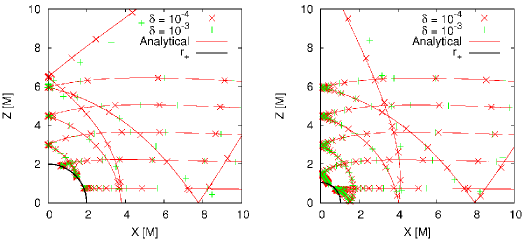
Figure 2: Geodesics of neutrinos in the ($r$-$\theta$) plane for the dimensionless Kerr parameter $a^{*}=0$ (left) and $a^{*}=0.999$ (right), obtained either analytically (lines) or numerically (points) with the two different regulation parameters ($\delta=10^{-4}$ (cross) and $10^{-3}$ (plus)) for the Runge-Kutta integration (e.g., section 2.1). The central black circle (quadrant) represents the event horizon of the BH. It is noted that the reflection at $X=0$ or $Z=0$ is just for a visualization. At $X=0$ for example, the rays continue to propagate left ($X<0$) in reality.

By a straightforward, albeit tedious calculation, one can obtain the well-known analytic form of the null geodesics in the ($r$-$\theta$) plane around a Kerr BH (e.g., Carter (1968); Bardeen et al. (1972); Cadez et al. (1998); Li et al. (2005)). Figure 2 shows the geodesics near the BH in the case of $a^{*}=0$ (left) or $a^{*}=0.999$ (right), obtained either numerically (points) or analytically (lines). In both cases, neutrinos are initially injected from the right edge of the figure with different impact parameters (for different $Z$ in the figure). They are shown to be dragged by the gravity of the BH, whose surface is indicated by the black line in the center. It is noted that the reflection at $X=0$ or $Z=0$ is just for a visualization. For example at $X=0$, the rays keep on propagating to the left ($X<0$) in reality. For the numerical solutions, we vary the two different parameters ($\delta=10^{-3},10^{-4}$), which regulate the numerical convergence in the adaptive integrator (see section 2.1). We find that the regulation parameter of $\delta=10^{-4}$ is sufficient to trace the trajectory in a good agreement with the analytic solution, which we take in the following calculations.

3.2 Geodesics in the ($r$-$\phi$) plane

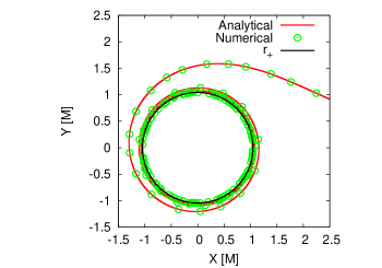
Figure 3: Same as Figure 2 but for the numerical solution (circle) in the (r-$\phi$) plane. $r_{+}$ indicates the position of the outer event horizon.

Now we move on to show the geodesics in the ($r$-$\phi$) plane. Since the analytical solution becomes very complicated in this case, we consider a special case that is $L=aE$ (Chandrasekhar, 1983). In this case, the evolution equations (Equations (16) - (19)) are greatly simplified as

$${\dot{r}} = \pm E,$$ (30)

$${\dot{\phi}} = \frac{aE}{\Delta}.$$ (31)

Combining these equations, the geodesics in the ($r$-$\phi$) plane becomes

$$\frac{d\phi}{dr} = \pm\frac{a}{\Delta},$$ (32)

$$\pm\phi = \frac{a}{r_{+}-r_{-}}\log\left(\frac{r}{r_{+}}-1\right)-\frac{a}{r_{+}-r_{-}}\log\left(\frac{r}{r_{-}}-1\right),$$ (33)

where $r_{\pm}$ is the position of the event horizon.

Figure 3 is the same as Figure 2, but for the geodesics in the ($r$-$\phi$) plane around an extremely rapidly rotating BH of $a^{*}=0.999$ (note again that $a^{*}=a/M$ is the dimensionless Kerr parameter). In the following, we call the case of $a^{*}=0.999$ as an extreme Kerr for simplicity. As shown, our numerical integration can reproduce the analytical solution without visible errors. These results support that our code can trace correctly the null geodesics in the Kerr geometry.

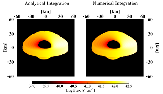
Figure 4: Comparison of the neutrino images around the accreting black holes with $a^{*}=0.999$, obtained either from the analytic (left) or numerical (right) integration of the geodesics. The neutrino flux shown is for the neutrino energy of $20{\rm MeV}$.

3.3 BH Shadow for Neutrinos

In this section, we demonstrate capability of our code to capture the imaging around the accreting black holes, which is often referred to as the BH shadow problem.

As for the neutrino sources, we assume a thin accretion disk with a Keplerian rotation profile. We set the mass of the BH to be $2M_{\odot}$ surrounded by the accretion disk, whose inner and outer radius are set to be the last stable orbit of the black hole ($r_{\rm lso}$) and $15GM/c^{2}$ with the disk thickness of $\pi/10$ (rad), respectively. The accretion disk is set to have a uniform density, temperature, and electron fraction of $10^{13}\,\,\mathrm{g\,\,cm^{-3}}$, $5\times 10^{11}{\rm K}$, and 0.3, respectively. We focus only on the electron-type neutrino in this test problem.

Figure 4 shows one example of the neutrino images around the accreting black holes seen from the viewing angle of $\theta_{\rm view}=72^{\circ}$ from the spin axis of the accretion disk. No visible differences are seen between the two panels, in which left and right panels are obtained either from the analytic or numerical integration of the geodesics. This supports the validity of our numerical integration of the rendering equation (Equation (28)).

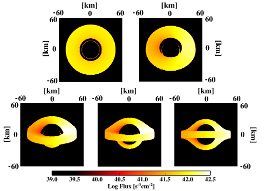
Figure 5: Neutrino images of the accretion disk for different viewing angles ($\theta_{\rm view}$ = $0^{\circ}$ (top left), $36^{\circ}$ (top right), from $72^{\circ}$, $81^{\circ}$ to $90^{\circ}$ (from bottom left to right). It is noted that $\theta_{\rm view}$ is the angle measured from the spin axis of the accretion disk. The spin parameter of central BH is set to be $a^{*}=0$.

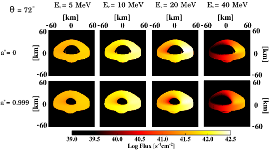
Figure 6: Images of the accretion disk for different neutrino energies ($E_{\nu}$) and BH spin parameters. The side length of each plot is 60 km.

Figure 5 shows a variety of the images seen from various viewing angles. For example, when we see the accretion disk from the equatorial plane (bottom right), we can observe neutrinos not only from the disk of the front side, but also from the opposite side because of the bending of the trajectory.

Figure 6 shows the images for different neutrino energies, while the viewing angle is kept fixed ($\theta_{\rm view}=72^{\circ}$). For lower energy neutrinos (such as for $5$ MeV (left panel)), the disk luminosity is shown to be almost north-south symmetric, while it becomes highly asymmetric for higher energy neutrinos (such as for $40$MeV (right panel)). As the neutrino energy becomes lower, the position of the neutrino sphere is formed deeper inside the accretion disk, by which we can see the regions closer to the BH (Figure 6). Since the angular velocity of the Keplerin disk is larger for the distant region from the center, the deformation of the images due to the Doppler effects can be more remarkably seen for the high energy neutrinos. It is interesting to note that in the case of the maximally rotating black hole (bottom panels), the BH shadow becomes asymmetric even for the low energy neutrinos due to the frame-dragging effects (bottom two left panels). Such features for the photon shadow in the vicinity of massive BHs in our Galactic center, have been considered to give an important information to reveal the mass and spin of the BHs (e.g., Takahashi & Watarai (2007); Nagakura & Takahashi (2010)). Although this may not be the case for GRBs due to their cosmological distances, the bending of neutrinos may have impacts on the gravitational radiation generated by anisotropic neutrino emission (e.g., Epstein (1978); Kotake et al. (2009a)). This can be one possible extension of this study.

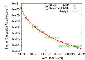
Figure 7: Comparison of the energy deposition rate from the spherical light-bulb test (see text for detail) for a given angular resolution of ray-tracing calculation ($n_{\theta}$ = 32) with or without the AMR treatment. Note in this test that we assume the Minkowskian geometry.

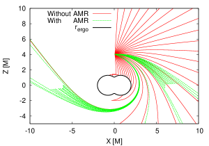
Figure 8: One example describing the casting of rays with (green) or without AMR technique (red). In this case, the rays are cast for estimating the annihilation rate at a given point (seen as a convergent point of the rays) outside the ergosphere ($r_{\rm ergo}$). The concentration of the rays is seen (green), which is helpful to correctly estimate the heating rates with reduced computational cost. Note in this figure that only selected rays are chosen for illustrative purpose. This plot is selected from the BH shadow problems (section 3.3) for the visualization of the AMR.

3.4 Neutrino Pair Annihilation from a Spherical Neutrino Sphere

For the collisional Boltzmann equation in GR, it is commonly not trivial to derive analytic solutions for a radiative transport problem. In the following, we derive the analytic solution for radiation fields, shedding from a spherical light-bulb into a uniform medium outside. We hope that the analytic solution may be useful to check newly developed codes for the radiative transport in curved space.

In the following numerical tests, the spherical neutrino sphere with a radius of $50\,\,\mathrm{km}$ is assumed to have its surface temperature of $T=5$ MeV on which the neutrino distribution function takes a Fermi-Dirac shape with vanishing chemical potential. The numerical domain [$50\,\,\mathrm{km}:300\,\,\mathrm{km}$] is covered with $n_{r}=100$ radial mesh points. The fiducial values of the energy and angular bins for the ray-tracing calculation are set to be $(n_{\epsilon^{\rm L}},n_{\theta},n_{\phi})=(16,32,16)$, which we will change to see the numerical convergence.

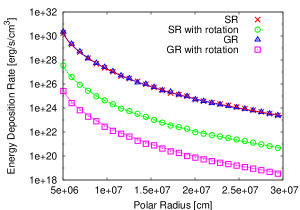
Figure 9: Same as Figure 7 but for the Minkowskian case with or without rotation (circle, cross), the Schwarzschild case with or without rotation (square, triangle). See text for detail. For models with rotation, we set $1/\sqrt{1-({\hat{v}}^{3})^{2}}=2$. For models with the Schwarzschild geometry, we put a point mass of $M=3M_{\odot}$ inside the neutrino sphere.

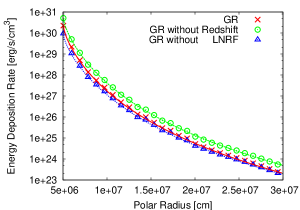
Figure 10: Same as Figure 7 but for the numerical solution without the gravitational redshift (circle), without the correction due to the tetrad transformation (triangle), and the one including both (cross). Agreement with the analytic solution (line) can be seen when the two ingredients are included (See text for detail.)

To find the analytic solution in Equation (3), we first take the most simplest case of $a^{*}=0,u^{r}=u^{\theta}=0$. In this case, the momenta $p^{\rm L}_{\alpha}$ in the LNRF can be expressed in the BLF as

$$p^{\rm L}_{\alpha}={\bar{\omega}}^{\beta}_{~{}\alpha}p_{\beta},$$ (34)

where

$${\bar{\omega}}^{\beta}_{~{}\alpha} \equiv (\omega^{\beta}_{~{}\alpha})^{-1}$$ (35)

$$= \begin{pmatrix}\frac{1}{\alpha}&0&0&0\\ 0&\frac{1}{\sqrt{\gamma_{rr}}}&0&0\\ 0&0&\frac{1}{\sqrt{\gamma_{\theta\theta}}}&0\\ -\frac{\beta^{\phi}}{\alpha}&0&0&\frac{1}{\sqrt{\gamma_{\phi\phi}}}\\ \end{pmatrix}.$$

In this way, the solid angle between the two frames can be readily shown to be the same ($d\Omega^{\rm L}=d\Omega$). Similarly, the volume element of the phase space and the neutrino energy in the local rest frame can be expressed by the variables in the BLF as follows,

$$d^{3}p^{\rm L} = -(p^{\rm L}_{0})^{2}dp^{\rm L}_{0}d\Omega^{\rm L}$$ (36)

$$= -({\bar{\omega}}^{0}_{0})^{3}(p_{0})^{2}dp_{0}d\Omega,$$

and

$$\epsilon^{\rm R} = -u^{\alpha}p_{\alpha}$$ (37)

$$= -u^{0}p_{0},$$

where

$$u^{0} = \frac{1}{\sqrt{-g_{\mu\nu}v^{\mu}v^{\nu}}}$$ (38)

$$= \frac{1}{\sqrt{-g_{00}-g_{33}(v^{3})^{2}}},$$

here we define $v^{\mu}=u^{\mu}/u^{0}$.

Inserting these results to Equation (3), we obtain the following analytic forms of the energy and momentum deposition rate respectively as,

$$Q_{t}^{\rm L}(\mbox{\boldmath$r$}) = 2cKG_{\rm F}^{2}\xi_{\nu}^{9}(\mbox{\boldmath$r$})E^{R}_{\nu}(\mbox{\boldmath$r$})N^{R}_{\nu}(\mbox{\boldmath$r$})F(\mbox{\boldmath$r$}),$$ (39)

$$Q_{r}^{\rm L}(\mbox{\boldmath$r$}) = 2cKG_{\rm F}^{2}\xi_{\nu}^{9}(\mbox{\boldmath$r$})E^{R}_{\nu}(\mbox{\boldmath$r$})N^{R}_{\nu}(\mbox{\boldmath$r$})G(\mbox{\boldmath$r$}).$$ (40)

Here $\xi_{\nu}$ reflects the general relativistic correction to the neutrino energy as

$$\xi_{\nu}(\mbox{\boldmath$r$}) \equiv \epsilon^{L}/\epsilon^{R}$$ (41)

$$= \sqrt{\frac{-g_{00}(R)-g_{33}(v^{3})^{2}}{-g_{00}(r)}}=\sqrt{\frac{1-2M/R-({\hat{v}}^{3})^{2}}{1-2M/r}},$$

where ${\hat{v}}^{3}=r\sin\theta~{}v^{3}$, and $R$ is the radius of the neutrino sphere. The following two quantities are the energy-weighted integration of the neutrino distribution function on the neutrino sphere (namely $f_{\nu}(\mbox{\boldmath$r$}_{\nu},\mbox{\boldmath$p$}_{\nu}^{R}$)) as,

$$E^{R}_{\nu}(\mbox{\boldmath$r$}) \equiv \int(\epsilon^{\rm R}_{\nu})^{4}f_{\nu}(\mbox{\boldmath$r$}_{\nu},\mbox{\boldmath$p$}^{\rm R}_{\nu})d\epsilon^{\rm R}_{\nu}$$ (42)

$$= \frac{(kT(\mbox{\boldmath$r$}_{\nu}))^{5}}{(hc)^{3}}{\cal F}_{4}(0),$$

$$N^{R}_{\nu}(\mbox{\boldmath$r$}) \equiv \int(\epsilon^{\rm R}_{\nu})^{3}f_{\nu}(\mbox{\boldmath$r$}_{\nu},\mbox{\boldmath$p$}^{R}_{\nu})d\epsilon^{\rm R}_{\nu}$$ (43)

$$= \frac{(kT(\mbox{\boldmath$r$}_{\nu}))^{4}}{(hc)^{3}}{\cal F}_{3}(0),$$

where $T(\mbox{\boldmath$r$}_{\nu})$ is set to be 5 MeV. Finally, geometrical factors of $F(r)$ and $G(r)$ are given as,

$$F(\mbox{\boldmath$r$}) \equiv \int\left[1-\sin{\theta_{\nu}}\sin{\theta_{\bar{\nu}}}\cos{(\varphi_{\nu}-\varphi_{\bar{\nu}})}-\cos{\theta_{\nu}}\cos{\theta_{\bar{\nu}}}\right]^{2}d\Omega_{\nu}d\Omega_{\bar{\nu}}$$ (44)

$$= \frac{2\pi^{2}}{3}(1-x^{4})(5+4x+x^{2}),$$

$$G(\mbox{\boldmath$r$}) \equiv \frac{\pi^{2}}{6}(1-x)^{4}(1+x)(8+9x+3x^{2}),$$ (45)

$$x \equiv \sqrt{1-\left(\frac{R}{r}\right)^{2}\frac{1-2M/r}{1-2M/R}}.$$ (46)

To emphasize the importance of AMR for our ray-tracing calculation (e.g., section 2.2), we first show Figure 7, in which we compare the energy deposition rates calculated with or without AMR treatment. A good agreement with the analytic solution can be obtained by utilizing the AMR technique. We take $n_{\theta}=32$ with AMR to be the fiducial value in the following test calculations. A visualization of AMR is also given in Figure 8.

In Figure 9, we compare the analytic solutions (line) with the corresponding numerical solutions in the following four cases; the Minkowskian case with or without rotation (circle, cross), the Schwarzschild case with or without rotation (square, triangle). For models with rotation, we set $1/\sqrt{1-({\hat{v}}^{3})^{2}}=2$. For models with the Schwarzschild geometry, we put a point mass of $M=3M_{\odot}$ inside the neutrino sphere. It is noted that analytic solutions for each case can be readily derived from Equation (39). In all the cases, the numerical solutions are shown to reproduce the corresponding analytic solutions quite well.

Here we present the test calculations to check our implementation of the two GR factors in Equation (41), that is the gravitational redshift ($-g_{00}(R)$) and the tetrad transformation ($-g_{00}(r)$). On purpose, we neglect each factor one by one, and compare it to the analytical solution. Figure 10 depicts the numerical solutions including both (cross) versus without the gravitational redshift (circle) or without the tetrad transformation (triangle). The analytic solutions (lines) are shown to be reproduced only when both of them are appropriately included.

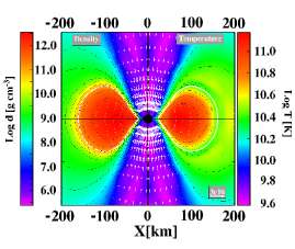
Figure 11: Hydrodynamic configuration employed in the ray-tracing calculation. This is the snapshot at 9.1 s after the onset of gravitational collapse for model J0.8 when the accretion disk is in a stationary state (see Harikae et al. (2010) for more detail). The logarithmic density (in$\,\,\mathrm{g\,\,cm^{-3}}$, left-half) and temperature (in $K$, right-half) are shown. The white solid line denotes the area where the density is equal to $10^{11}\,\,\mathrm{g\,\,cm^{-3}}$, representing the surface of the accretion disk. The central black circle ($\approx 4M_{\odot}$) represents the inner boundary of our computations.

4 Application to Collapsar Model

Having checked the accuracy of our code in previous sections, we are now in a position to show an application of our code in the collapsar’s environment. As in Harikae et al. (2010), we estimate the annihilation rates in a post-processing manner using the hydrodynamic data obtained in our long-term collapsar simulations. By comparing the neutrino-heating timescale to the advection timescale of material in the polar funnel regions (see Harikae et al. (2010) for detail), we discuss the possibility of generating neutrino-driven outflows there. Paying particular attention to the GR effects on the annihilation rates, we discuss their possible impacts on the collapsar dynamics.

As for the hydrodynamic data (such as density, electron fraction, and entropy), we take the ones at 9.1 s after the onset of gravitational collapse for model J0.8 (Figure 11), which show a clear accretion-disk and BH system with the polar funnel regions along the spin axis of the disk. Since this model is calculated by special relativistic hydrodynamics, we project those data into the ones in the LNRF for the ray-tracing calculation. The position of the inner boundary of the computational domain is set to be $4M_{\odot}$, which mimics the event horizon of the BH. We set the Kerr parameter by hand as $a^{*}=0$ for the Schwarzschild geometry and $a^{*}=0.999$ for the extreme Kerr geometry.

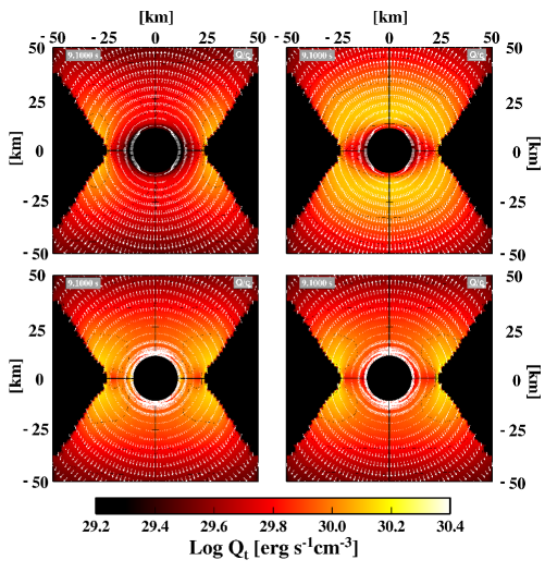
Figure 12: Logarithmic contour of energy deposition rates $Q_{t}\,[{\rm erg}~{}{\rm s}^{-1}~{}{\rm cm}^{-3}]$ and normalized vector of momentum deposition rates $Q_{i}/Q_{t}$ calculated for the Minkowskian geometry (top left/top right:without/with special relativistic corrections), the Schwarzschild geometry (bottom left), and the extreme Kerr geometry ($a^{*}=0.999$) (bottom right). The spatial vector is visualized by showing the spatial velocity vector $v\equiv Q_{i}/Q_{t}$, which is normalized by the speed of light $(c=1)$ being represented by the arrow (top right in each panel). The central black circle ($\approx 4M_{\odot}$) represents the inner boundary of the computational domain. Note that the triangular regions colored by black closely coincide the surface of the accretion disk (e.g., Figure 11).

4.1 Effect of General Relativity on Energy and Momentum Deposition

To clarify the GR effects, we compare the annihilation rates in the Minkowkian ($M=0$), Schwarzschild, and extreme Kerr geometry ($a^{*}=0.999$). Figure 12 shows the energy deposition rate $Q_{t}$ (contour) (Equation 3) and the normalized momentum transfer rate $Q_{i}/Q_{t}$ (vector) (e.g., Equation 3) for the Minkowskian geometry (top left/top right: with/without special relativistic corrections), the Schwarzschild geometry (bottom left), and the extreme Kerr geometry (bottom right), respectively. And Figure 13 is a difference plot, which shows the energy deposition rate normalized by the one in the Minkowskian geometry (top left in Figure 12).

From Figure 12, it can be seen in the Minkowskian geometry (top two panels) that the direction of the momentum transfer is generally radially outward, while in the Schwarzschild and Kerr geometry (bottom two panels), the direction especially in the vicinity of the BH tends to direct the center as a result of the general relativistic bending. This bending effect, acting to suppress the outward momentum transfer, should do harm to launch the neutrino-driven outflow. On the other hand, it does good to the energy deposition, because it enhances the head-on collision especially in the polar funnel regions.

In fact, it can be seen that the deposition rate for the Schwarzschild and Kerr geometry becomes larger than for the Minkowskian geometry (Figure 13). In the blueish region that corresponds to the polar funnel region, the energy deposition rate for the extreme Kerr geometry is enhanced by factors compared to the Minkowskian geometry. Interestingly it is mentioned that the heating rate is enhanced by about one order-of-magnitude near the equatorial plane in the vicinity of the BH. This is because the neutrino rays are concentrated there, reflecting the conical shape of the accretion disk (triangular blackish regions at the sides). This concentration near the equatorial plane is found to be suppressed for the maximally rotating BH mainly due to the frame-dragging effect.

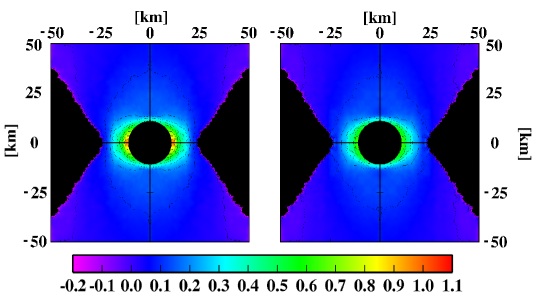
Figure 13: Difference plot which shows the energy deposition rate in the Schwarzschild (left) and extreme Kerr geometry (right), which are normalized by the one in the Minkowskian geometry (see top left in Figure 12).

To see the GR effects on the net energy deposition, we calculate the total energy deposition rate,

$$Q^{\rm tot}_{\nu{\bar{\nu}}}=\int\sqrt{-g}Q_{t}dV,$$ (47)

and the one with the outgoing momentum as Jaroszynski (1993); Birkl et al. (2007))

$$Q^{\rm out}_{\nu{\bar{\nu}}}=\left.\int\sqrt{-g}Q_{t}dV\right|_{Q_{r}>0},$$ (48)

where the contributions with the outgoing radial component of the momentum vector ($Q_{r}$) are counted. As shown in Table 1, the net deposition rate and efficiency for the extreme Kerr geometry increase up to $16\%$ ($18\%$ for $Q^{\rm out}_{\nu{\bar{\nu}}}$) compared to the Minkowskian geometry. Our results support the previous study that GR can enhance the heating rate, and thus good for the formation of the neutrino-driven outflow (e.g., Birkl et al. (2007)). From Table 1, the deposition rate and efficiency are barely influenced by the spin of BH. However it should be noted that we have included the spin effects only in the radiative transport. As pointed out by Asano & Fukuyama (2001); Birkl et al. (2007), the spin effects, such as on the structure of the spacetime (i.e., the inner-most stable circular orbit becomes smaller for the rapidly rotating black hole) and also on the accretion disk, should be more important to affect the heating rate. To clarify this point, we need a hydrodynamic data based on the general relativistic simulations of collapsars, which we are to investigate as a sequel of this study.

Geometry	$Q^{\rm tot}_{\nu{\bar{\nu}}}[{\rm erg\,\,s^{-1}}]$	$Q^{\rm out}_{\nu{\bar{\nu}}}[{\rm erg\,\,s^{-1}}]$	efficiency [%]
Minkowski	$6.18\times 10^{50}$	$5.71\times 10^{50}$	0.510
Schwarzschild	$7.15\times 10^{50}$	$6.09\times 10^{50}$	0.590
Extreme Kerr	$7.08\times 10^{50}$	$6.13\times 10^{50}$	0.585

Table 1: Comparison of $Q_{\nu{\bar{\nu}}}^{\rm tot}$, $Q_{\nu{\bar{\nu}}}^{\rm out}$ (see Equations (47,48)) and efficiency for the Minkowskian, Schwarzschild, and extreme Kerr ($a^{*}=0.999$) geometry, which corresponds to the top left, bottom left and right panels in Figure 12, respectively. Efficiency is evaluated as $Q^{\rm tot}_{\nu{\bar{\nu}}}/L_{\nu}$ where $L_{\nu}$ is the total neutrino luminosity.

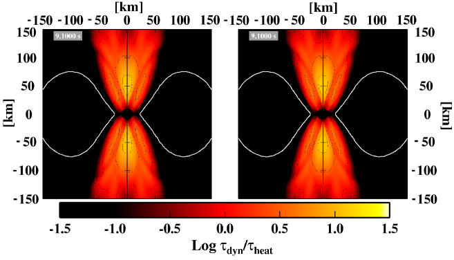
Figure 14: Same as Figure 12 but for $\tau_{\rm dyn}/\tau_{\rm heat}$ (:the dynamical timescale $\tau_{\rm dyn}$ versus the heating timescale $\tau_{\rm heat}$) in the Schwarzschild (left) and extreme Kerr geometry (left), respectively.

4.2 Condition for Outflow Formation

Based on the annihilation rates in the last section, we compare the two timescales in this section, which are the neutrino-heating timescale and the dynamical timescale. Then we anticipate if the neutrino-heating outflows could or could not be produced in the polar funnel regions.

To trigger the neutrino-heating explosion, the neutrino-heating timescale should be smaller than the advection timescale, which is characterised by the free-fall timescale in the polar funnel regions. This condition is akin to the condition of the successful neutrino-driven explosion in the case of core-collapse supernovae (e.g., Bethe (1990) and see collective references in Janka et al. (2007)). The heating timescale is the timescale for a fluid to absorb the energy by the neutrino heating, comparable to the gravitational binding energy for making the fluid gravitationally unbound, which may be defined as $\tau_{\rm{heat}}\equiv\rho\Phi/Q_{t}$. Here $\Phi$, the local gravitational potential, is taken to be the sum of the pseudo-Newtonian potential and self-gravity in the flat space-time (Harikae et al., 2010) and $\rho$ is the local matter density. Then the dynamical timescale is defined as $\tau_{\rm{dyn}}\equiv\sqrt{3\pi/16G\bar{\rho}}$, where $\bar{\rho}$ is the average density at a certain radius and we take $\bar{\rho}(r)\equiv 3M(r)/4\pi r^{3}$.

Figure 14 depicts the ratio of the dynamical $\tau_{\rm{dyn}}$ to the heating timescales $\tau_{\rm{heat}}$ for the Schwarzschild (left) and extreme Kerr geometry (right), showing in both cases that the ratio becomes greater than unity in the polar funnel regions (compare Figure 11). Figure 15 shows the energy deposition rate along the polar axis of Figure 12, for the Minkowskian geometry without or with the special relativistic correction (indicated by “Newtonian” and “SR”), and for the Schwarzschild and extreme Kerr geometry (indicated by “GR ($a^{*}=0$)” and “GR ($a^{*}=0.999$)”). It is noted that the energy deposition sharply drops from the Newtonian to the SR case (left panel). This is the outcome of the special relativistic beaming effects. Since the rotational velocity of the accretion disk is perpendicular to the polar direction, the special relativistic beaming effect suppresses the neutrino emission toward the polar region. (see Harikae et al. (2010) for more detail). When the general relativistic bending effects are taken into account, the deposition rate becomes larger again (see “GR ($a^{*}=0$)” and “GR ($a^{*}=0.999$)”). Reflecting this situation, $\tau_{\rm dyn}/\tau_{\rm heat}$ becomes smallest for the case with SR and largest for the Newtonian case (right panel of Figure 15). It is important that the ratio in the case of the Schwarzschild and extreme Kerr geometry, which do reflect nature in the collapsar’s environment, becomes larger than unity inside 100 km in the vicinity of the rotational axis (Figure 15, right). This indicates the possible formation of the neutrino-driven outflows there, if coupled to the collapsar’s hydrodynamics.

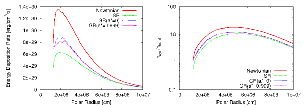
Figure 15: Comparison of energy deposition rate (left) and $\tau_{\rm dyn}/\tau_{\rm heat}$ along the rotational axis (right) between the Minkowskian geometry without or with the special relativistic correction (indicated by “Newtonian” and “SR”), and for the Schwarzschild and extreme Kerr geometry (indicated by “GR ($a^{*}=0$)” and “GR ($a^{*}=0.999$)”).

5 Summary and Discussion

In the light of collapsar models of gamma-ray bursts (GRBs), we developed a numerical scheme and code for estimating the deposition of energy and momentum due to the neutrino pair annihilation ($\nu+{\bar{\nu}}\rightarrow e^{-}+e^{+}$) in the vicinity of accretion tori around a Kerr black hole. We designed our code to calculate the general relativistic neutrino transfer by a ray-tracing method. To solve the collisional Boltzmann equation in the Kerr geometry, we numerically integrated the so-called rendering equation along the null geodesics. For the neutrino opacity, the charged-current $\beta$-processes are taken into account, which are dominant in the vicinity of the accretion tori. We employed the Fehlberg(4,5) adaptive integrator in the Runge-Kutta method in order to perform the numerical integration accurately. We checked the numerical accuracy of the developed code by several tests, in which we showed comparisons with the corresponding analytical solutions. In order to solve the energy dependent ray-tracing transport, we proposed that an adaptive-mesh-refinement approach, which we took for the two radiation angles $(\theta,\phi)$ and the neutrino energy, is efficient to reduce the computational cost. Based on the hydrodynamical data in our collapsar simulation, we estimated the annihilation rates in a post-processing manner. It is found that the general relativistic effect can increase the local energy deposition rate by about one order of magnitude, and the net energy deposition rate by several tens of percents. After the accretion disk settles into a stationary state (typically later than $\sim 9$ s from the onset of gravitational collapse), we pointed out that the neutrino-heating timescale can be smaller than the dynamical timescale inside 100 km in the vicinity of the rotational axis. Our results suggest that the neutrino-driven outflows can possibly be launched there.

For further investigation, we need to include several important ingredients ignored in this study. We plan to develop a GRMHD code for collapsars, which is indispensable to see the outcome of this paper. By changing the precollapse magnetic fields and rotation systematically, we hope to clearly understand how the outflow formation in collapsars could change from the neutrino-driven mechanism to the MHD-driven one. The neutrino oscillation by the Mikheyev-Smirnov-Wolfenstein (MSW) effect (see collective references in Kotake et al. (2006); Kawagoe et al. (2009)) could be important, albeit in much later phase than we considered in this paper. When the density in the polar funnel regions drops as low as $\rho\lesssim 10^{3}\,\,\mathrm{g\,\,cm^{-3}}$ later, the neutrino oscillation could operate for neutrinos traveling from the accretion disk to the polar funnel. If this is the case, the incoming neutrino spectra to the polar funnel regions and the pair annihilation rates there could be affected significantly. It is also noted that the effects of neutrino self-interaction are remained to be studied, which has been attracting great attention in the theory of core-collapse supernovae (e.g., Duan et al. (2006)). As in the case of core-collapse supernovae (e.g., Kotake et al. (2009b); Ott et al. (2008b)), studies of gravitational-wave emissions from collapsars might provide us a new window to probe into the central engine (e.g., Hiramatsu et al. (2005); Suwa & Murase (2009)). As a sequel of this work, we are planning to implement the ray-tracing calculation to the GRMHD simulation and clarify these issues one by one. We hope that this study takes a very first step towards the meeting of GR with neutrino transport, which should be indispensable for understanding the collapsar engines.

References

- Aloy et al. (2000) Aloy, M. A., Müller, E., Ibáñez, J. M., Martí, J. M., & MacFadyen, A. 2000, ApJ, 531, L119
- Asano & Fukuyama (2000) Asano, K. & Fukuyama, T. 2000, ApJ, 531, 949
- Asano & Fukuyama (2001) —. 2001, ApJ, 546, 1019
- Bardeen et al. (1972) Bardeen, J. M., Press, W. H., & Teukolsky, S. A. 1972, ApJ, 178, 347
- Barkov & Komissarov (2008) Barkov, M. V. & Komissarov, S. S. 2008, MNRAS, 385, L28
- Bethe (1990) Bethe, H. A. 1990, Reviews of Modern Physics, 62, 801
- Birkl et al. (2007) Birkl, R., Aloy, M. A., Janka, H.-T., & Müller, E. 2007, A&A, 463, 51
- Blandford & Znajek (1977) Blandford, R. D. & Znajek, R. L. 1977, MNRAS, 179, 433
- Bruenn (1985) Bruenn, S. W. 1985, ApJS, 58, 771
- Cadez et al. (1998) Cadez, A., Fanton, C., & Calvani, M. 1998, New Astronomy, 3, 647
- Carter (1968) Carter, B. 1968, Physical Review, 174, 1559
- Chandrasekhar (1983) Chandrasekhar, S. 1983, The mathematical theory of black holes (Oxford University Press)
- Cunningham (1975) Cunningham, C. T. 1975, ApJ, 202, 788
- Cunningham & Bardeen (1973) Cunningham, J. M. & Bardeen, C. T. 1973, ApJ, 183, 237
- Dessart et al. (2009) Dessart, L., Ott, C. D., Burrows, A., Rosswog, S., & Livne, E. 2009, ApJ, 690, 1681
- Duan et al. (2006) Duan, H., Fuller, G. M., & Qian, Y.-Z. 2006, Phys. Rev. D, 74, 123004
- Epstein (1978) Epstein, R. 1978, ApJ, 223, 1037
- Fanton et al. (1997) Fanton, C., Calvani, M., de Felice, F., & Cadez, A. 1997, PASJ, 49, 159
- Fehlberg, E. (1970) Fehlberg, E. 1970, j-COMPUTING, 6, 61
- Fujimoto et al. (2006) Fujimoto, S.-i., Kotake, K., Yamada, S., Hashimoto, M.-a., & Sato, K. 2006, ApJ, 644, 1040
- Fuller et al. (1985) Fuller, G. M., Fowler, W. A., & Newman, M. J. 1985, ApJ, 293, 1
- Goodman et al. (1987) Goodman, J., Dar, A., & Nussinov, S. 1987, ApJ, 314, L7
- Harikae et al. (2010) Harikae, S., Kotake, K., & Takiwaki, T. 2010, ApJ, 713, 304
- Harikae et al. (2009) Harikae, S., Takiwaki, T., & Kotake, K. 2009, ApJ, 704, 354
- Hiramatsu et al. (2005) Hiramatsu, T., Kotake, K., Kudoh, H., & Taruya, A. 2005, MNRAS, 364, 1063
- Janka et al. (2007) Janka, H., Langanke, K., Marek, A., Martínez-Pinedo, G., & Müller, B. 2007, Phys. Rep., 442, 38
- Janka & Hillebrandt (1989) Janka, H.-T. & Hillebrandt, W. 1989, A&AS, 78, 375
- Jaroszynski (1993) Jaroszynski, M. 1993, Acta Astronomica, 43, 183
- Jaroszynski (1996) —. 1996, A&A, 305, 839
- Kawagoe et al. (2009) Kawagoe, S., Takiwaki, T., & Kotake, K. 2009, Journal of Cosmology and Astro-Particle Physics, 9, 33
- Komissarov & Barkov (2007) Komissarov, S. S. & Barkov, M. V. 2007, MNRAS, 382, 1029
- Kotake et al. (2009a) Kotake, K., Iwakami, W., Ohnishi, N., & Yamada, S. 2009a, ApJ, 704, 951
- Kotake et al. (2009b) —. 2009b, ApJ, 697, L133
- Kotake et al. (2006) Kotake, K., Sato, K., & Takahashi, K. 2006, Reports on Progress in Physics, 69, 971
- Li et al. (2005) Li, L., Zimmerman, E. R., Narayan, R., & McClintock, J. E. 2005, ApJS, 157, 335
- Lindquist (1966) Lindquist, R. W. 1966, Annals of Physics, 37, 487
- Lyutikov (2006) Lyutikov, M. 2006, New Journal of Physics, 8, 119
- MacFadyen & Woosley (1999) MacFadyen, A. I. & Woosley, S. E. 1999, ApJ, 524, 262
- McKinney & Narayan (2007) McKinney, J. C. & Narayan, R. 2007, MNRAS, 375, 513
- Meszaros & Rees (1992) Meszaros, P. & Rees, M. J. 1992, MNRAS, 257, 29P
- Misner & Sharp (1964) Misner, C. W. & Sharp, D. H. 1964, Physical Review, 136, 571
- Misner et al. (1973) Misner, C. W., Thorne, K. S., & Wheeler, J. A. 1973, Gravitation (San Francisco: W.H. Freeman and Co.)
- Mizuno et al. (2004) Mizuno, Y., Yamada, S., Koide, S., & Shibata, K. 2004, ApJ, 615, 389
- Mizuta & Aloy (2009) Mizuta, A. & Aloy, M. A. 2009, ApJ, 699, 1261
- Müller & Camenzind (2004) Müller, A. & Camenzind, M. 2004, A&A, 413, 861
- Nagakura & Takahashi (2010) Nagakura, H. & Takahashi, R. 2010, ArXiv e-prints
- Nagataki (2009) Nagataki, S. 2009, ApJ, 704, 937
- Nagataki et al. (2007) Nagataki, S., Takahashi, R., Mizuta, A., & Takiwaki, T. 2007, ApJ, 659, 512
- Ott et al. (2008a) Ott, C. D., Burrows, A., Dessart, L., & Livne, E. 2008a, ApJ, 685, 1069
- Ott et al. (2008b) —. 2008b, ApJ, 685, 1069
- Paczynski (1990) Paczynski, B. 1990, ApJ, 363, 218
- Paczynski (1998) —. 1998, ApJ, 494, L45+
- Papageorgiou et al. (1988) Papageorgiou, G., Simos, T., & Tsitouras, C. 1988, Celestial Mechanics, 44, 167
- Piro et al. (1998) Piro, L., Amati, L., Antonelli, L. A., Butler, R. C., Costa, E., Cusumano, G., Feroci, M., Frontera, F., Heise, J., in ’t Zand, J. J. M., Molendi, S., Muller, J., Nicastro, L., Orlandini, M., Owens, A., Parmar, A. N., Soffitta, P., & Tavani, M. 1998, A&A, 331, L41
- Proga (2003) Proga, D.and Begelman, M. C. 2003, ApJ, 592, 767
- Rauch & Blandford (1994) Rauch, K. P. & Blandford, R. D. 1994, ApJ, 421, 46
- Ruffert & Janka (1998) Ruffert, M. & Janka, H.-T. 1998, A&A, 338, 535
- Ruffert et al. (1997) Ruffert, M., Janka, H.-T., Takahashi, K., & Schaefer, G. 1997, A&A, 319, 122
- Salmonson & Wilson (1999) Salmonson, J. D. & Wilson, J. R. 1999, ApJ, 517, 859
- Shibata et al. (2007) Shibata, M., Sekiguchi, Y., & Takahashi, R. 2007, Progress of Theoretical Physics, 118, 257
- Suwa & Murase (2009) Suwa, Y. & Murase, K. 2009, Phys. Rev. D, 80, 123008
- Takahashi et al. (1978) Takahashi, K., El Eid, M. F., & Hillebrandt, W. 1978, A&A, 67, 185
- Takahashi (2004) Takahashi, R. 2004, ApJ, 611, 996
- Takahashi (2005) —. 2005, PASJ, 57, 273
- Takahashi & Watarai (2007) Takahashi, R. & Watarai, K. 2007, MNRAS, 374, 1515
- Takiwaki et al. (2009) Takiwaki, T., Kotake, K., & Sato, K. 2009, ApJ, 691, 1360
- Thompson et al. (2004) Thompson, T. A., Chang, P., & Quataert, E. 2004, ApJ, 611, 380
- Tubbs (1978) Tubbs, D. L. 1978, ApJS, 37, 287
- Uzdensky & MacFadyen (2007) Uzdensky, D. A. & MacFadyen, A. I. 2007, ApJ, 669, 546
- Čadež et al. (2003) Čadež, A., Brajnik, M., Gomboc, A., Calvani, M., & Fanton, C. 2003, A&A, 403, 29
- Čadež & Calvani (2005) Čadež, A. & Calvani, M. 2005, MNRAS, 363, 177
- Čadež & Kostić (2005) Čadež, A. & Kostić, U. 2005, Phys. Rev. D, 72, 104024
- Woosley (1993) Woosley, S. E. 1993, ApJ, 405, 273
- Woosley & Bloom (2006) Woosley, S. E. & Bloom, J. S. 2006, ARA&A, 44, 507
- Zhang et al. (2003) Zhang, W., Woosley, S. E., & MacFadyen, A. I. 2003, ApJ, 586, 356
- Zink (2008) Zink, B. 2008, Ray-tracing Black Holes (VDM Verlag)