Occupation time distributions for the telegraph process

Abstract

For the one-dimensional telegraph process, we obtain explicit distribution of the occupation time of the positive half-line. The long-term limiting distribution is then derived when the initial location of the process is in the range of sub-normal or normal deviations from the origin; in the former case, the limit is given by the arcsine law. These limit theorems are also extended to the case of more general occupation-type functionals.

1 Introduction

Let $B=(B_{t},\,t\geq 0)$ be a standard Brownian motion on $\mathbb{R}$ starting from the origin ($B_{0}=0$), and consider the occupation time functional

$${\mathfrak{h}}_{T}:=\frac{1}{T}\int_{0}^{T}H(B_{t})\,{\rm d}t,\qquad T>0,$$ (1.1)

where $H(x)$ is the Heaviside unit step function (i.e., $H(x)=0$ for $x\leq 0$ and $H(x)=1$ for $x>0$). That is to say, ${\mathfrak{h}}_{T}\in[0,1]$ is the proportion of time spent by the Brownian motion $(B_{t},\ 0\leq t\leq T)$ on the positive half-line. It is well known that the probability distribution of the random variable ${\mathfrak{h}}_{T}$ does not depend on $T$ (which is evident from the scaling property of the Brownian motion and the fact that $H(\alpha x)\equiv H(x)$ for any $\alpha>0$) and is given by the classic arcsine law,

$$\mathbb{P}\{{\mathfrak{h}}_{T}\leq y\}=\frac{2}{\pi}\arcsin\sqrt{y},\qquad 0\leq y\leq 1,$$ (1.2)

with the probability density

$$p_{\mathrm{as}}(y):=\frac{1}{\pi\sqrt{y\mbox{$\>\!$}(1-y)}}\,,\qquad 0<y<1.$$ (1.3)

The beautiful formula (1.2) dates back about 70 years to P. Lévy [Le40, Théorème 3, pp. 301–302], who has also proved that the arcsine law (1.2) is the limit distribution for the relative frequency of positive sums among consecutive partial sums of independent symmetric Bernoulli ($0\text{--}1$) random variables [Le40, Corollaire 2, p. 303]. Using the invariance principle, the latter result was extended by P. Erdős and M. Kac [EKa47] to the case of sums of arbitrary i.i.d. random variables with zero mean and unit variance (cf. [St93, Theorem 4.3.19, p. 236]). More recently, R. Khasminskii [Kh99] obtained the limit distribution, as $T\to\infty$, of more general functionals of the form

$${\mathfrak{h}}_{T}(x;f):=\frac{1}{T}\int_{0}^{T}f(x+X_{t})\,{\rm d}t,$$

where $(X_{t},\,t\geq 0)$ is a diffusion process on $\mathbb{R}$ ($X_{0}=0$) with generator $L=-a(x)\,{\rm d}^{2}/{\rm d}x^{2}$, and $f:\mathbb{R}\to\mathbb{R}$ is a probing function from a suitable class. In particular, the results of [Kh99] imply that if $\lim_{x\to\pm\infty}a(x)=a_{0}>0$ and $f$ is a bounded piecewise continuous function such that

$$\lim_{x\to\pm\infty}\frac{1}{x}\int_{0}^{x}f(u)\,{\rm d}{u}=f_{\pm}\,,\qquad f_{+}\neq f_{-}\,,$$ (1.4)

then the distribution of the random variable $({\mathfrak{h}}_{T}(x;f)-f_{-})/(f_{+}-f_{-})$ converges weakly, as $T\to\infty$, to the arcsine law (1.2).

In the present paper, we obtain similar results for the so-called telegraph process defined by

$$X_{t}:=V_{0}\int_{0}^{t}(-1)^{N_{u}}\,{\rm d}u,\qquad t\geq 0,$$ (1.5)

where $(N_{t},\,t\geq 0)$ is a homogeneous Poisson process (with rate $\lambda>0$), $V_{0}$ is a random variable with equiprobable values $\pm c$ independent of the process $N_{t}$, and $c>0$ is a parameter (see [Go51, Ka74, Pi91]). That is, $X_{t}$ is the position at time $t\geq 0$ of a particle starting at $t=0$ from the origin and moving on the line with alternating velocities $\pm c$, reversing the direction of motion at each jump instant of the Poisson process $N_{t}$; the initial (random) direction is decided by the sign of $V_{0}$. Note that the process $X_{t}$ itself is non-Markovian, however if $V_{t}={\rm d}X_{t}/{\rm d}{t}=(-1)^{N_{t}}\mbox{$\>\!$}V_{0}$ is the corresponding velocity process, then the joint process $(X_{t},V_{t})$ is Markov on the state space $\mathbb{R}\times\{-c,+c\}$ (see [EtK86, § 12.1, p. 469]). We shall also consider the conditional telegraph processes obtained from $X_{t}$ by conditioning on $V_{0}$,

$$X_{t}^{\pm}:=\pm\mbox{$\;\!$}c\int_{0}^{t}(-1)^{N_{u}}\,{\rm d}u,\qquad t\geq 0,$$ (1.6)

where the choice of the $+$ or $-$ sign determines the initial direction of motion.

Remark 1.1.

Here and throughout the paper, we adopt a notational convention that any formula involving the $\pm$ and $\mp$ signs combines the two cases corresponding to the choice of either the upper or lower sign, respectively.

Remark 1.2.

The telegraph process is the simplest example of so-called random evolutions (see, e.g., [EtK86, Ch. 12] and [Pi91, Ch. 2]).

The model of non-interacting particles moving in one dimension with alternating velocities (updated at random on a discrete time grid) was first introduced in 1922 by G. I. Taylor [Ta22] in an attempt to describe turbulent diffusion; later on (around 1938–1939) it was studied at length by S. Goldstein [Go51] in connection with a certain hyperbolic partial differential equation (called the telegraph, or damped wave equation, see (1.7) below) describing the spatio-temporal dynamics of the potential in a transmitting cable (without leakage) [We55]. In his 1956 lecture notes, M. Kac (see [Ka74]) considered a continuous-time version of the telegraph model. Since then, the telegraph process and its many generalizations have been studied in great detail (see, e.g., [Or90, Pi91, Or95, Ra99, We02]), with numerous applications in physics [We02], biology [Ha99, HH05], ecology [OL01] and, more recently, financial market modelling [Ra07, RM08] (see also further bibliography in these papers).

An efficient conventional approach to the analytical study of the telegraph process, analogous to that for diffusion processes, is based on pursuing a fundamental link relating various expected values of the process with initial value and/or boundary value problems for certain partial differential equations (see, e.g., [Go51, Or90, Or95, Ra97, Ra99, Ra06]). In particular, Kac [Ka74] has shown that, for any bounded continuously differentiable function $g_{0}:\mathbb{R}\to\mathbb{R}$, the functions

$$v^{\pm}(x,t):=\mathbb{E}\bigl{[}g_{0}(x+X^{\pm}_{t})\bigr{]},\qquad x\in\mathbb{R},\ t\geq 0,$$

satisfy the set of partial differential equations

$$\frac{\partial v^{\pm}(x,t)}{\partial t}\mp c\,\frac{\partial v^{\pm}(x,t)}{\partial x}=\mp\lambda\left(v^{+}(x,t)-v^{-}(x,t)\right),\qquad t>0,$$

with the initial conditions

$$v^{\pm}(x,0)=g_{0}(x),\qquad x\in\mathbb{R}.$$

These equations can be easily combined (see details in [Ka74] or [EtK86, § 12.1, p. 470]) to show that the function

$$v(x,t):=\mathbb{E}\left[g_{0}(x+X_{t})\right]=\frac{1}{2}\,v^{-}(x,t)+\frac{1}{2}\,v^{+}(x,t)$$

satisfies the telegraph (or telegrapher’s) equation (see, e.g., [We55, § 15])

$$\frac{\partial^{2}v}{\partial t^{2}}+2\lambda\frac{\partial v}{\partial t}=c^{2}\frac{\partial^{2}v}{\partial x^{2}}\,$$ (1.7)

with the initial conditions

$$v(x,0)=g_{0}(x),\qquad\frac{\partial v}{\partial t}(x,0)=0\mbox{$\>\!$}.$$ (1.8)

Remark 1.3.

The telegraph equation (1.7) first appeared more than 150 years ago in work by W. Thomson (Lord Kelvin) on the transatlantic cable [Th54].

The (unique) solution of the Cauchy problem (1.7) – (1.8) can be written explicitly (see, e.g., [We55, §§ 46, 74] or [Pi91, § 0.4]) as

$$v(x,t) =\frac{1}{2}\,{\rm e}^{-\lambda t}\bigl{(}g_{0}(x+ct)+g_{0}(x-ct)\bigr{)}$$ (1.9)

$$\quad+\frac{1}{2}\,{\rm e}^{-\lambda t}\int_{-t}^{t}g_{0}(x+cu)\left(\lambda I_{0}\bigl{(}\lambda\sqrt{t^{2}-u^{2}}\,\bigr{)}+\frac{\lambda\mbox{$\>\!$}t}{\sqrt{t^{2}-u^{2}}}\,I_{1}\bigl{(}\lambda\sqrt{t^{2}-u^{2}}\bigr{)}\right){\rm d}{u}\mbox{$\>\!$},$$

where

$$I_{0}(z):=\sum_{n=0}^{\infty}\frac{(z/2)^{2n}}{(n!)^{2}}\ \ \quad\text{and}\ \ \quad I_{1}(z):=I_{0}^{\prime}(z)=\frac{z}{2}\sum_{n=0}^{\infty}\frac{(z/2)^{2n}}{n!\,(n+1)!}\qquad(z\in\mathbb{R})$$

are the modified Bessel functions of the first kind (of orders $0$ and $1$), respectively) [AS72, 9.6.12, p. 375; 9.6.27, p. 376].

It is well known that, under a suitable scaling, the telegraph process satisfies a functional central limit theorem.

Theorem 1.1.

Assume that $\lambda,\mbox{$\>\!$}{}c\to+\infty$ in such a way that $c^{2}\mbox{$\;\!\!$}/\lambda\to 1$. Then the distribution of the telegraph processes $(X^{\pm}_{t},\,t\geq 0)$ converges weakly in $C[0,\infty)$ to the distribution of a standard Brownian motion $(B_{t},\,t\geq 0)$. The same is true for the unconditional telegraph process $(X_{t},\,t\geq 0)$.

As was observed by Kac [Ka74, p. 501], this result formally follows from the telegraph equation (1.7), which in the limit $\lambda,\mbox{$\;\!$}{}c\to+\infty$,  $c^{2}\mbox{$\;\!\!$}/\lambda\to 1$ yields the diffusion (heat) equation

$$\frac{\partial v}{\partial t}=\frac{1}{2}\,\frac{\partial^{2}v}{\partial x^{2}}\,,$$

associated with the standard Brownian motion $B_{t}$. A rigorous proof of Theorem 1.1, along with some extensions, can be found in [EtK86, § 12.1, p. 471] and [Ra99, Theorem 5.1].

Our main goal in the present paper is to analyze the distribution of the occupation time of the telegraph process $X_{t}$ and, in particular, to obtain a limit distribution, as $T\to\infty$, of the occupation-type functionals of the form $\eta_{T}(x;f):=T^{-1}\!\int_{0}^{T}f(x+X_{t})\,{\rm d}t$ for a suitable class of probing functions $f$. In particular, we prove that the limit distribution is given by Lévy’s arcsine law providing that the starting point $x$ is in the range of subnormal deviation from the origin (i.e., $x=o(\sqrt{T}\,)$). For technical simplicity, we impose a stronger condition on the asymptotics of $f$ at $\pm\infty$, assuming that the corresponding limits $f_{\pm}$ exist.

The rest of the paper is organized as follows. In Section 2 we state the main results of this work (Theorems 2.1 – 2.4), which are then proved in Sections 4 – 7, respectively. Section 3 contains a suitable version of the Feynman–Kac formula, with applications to the Laplace transforms for the occupation-type functionals under study, which is instrumental for our techniques. We finish in Section 8 with concluding remarks and some conjectures, which are illustrated by the results of computer simulations. Appendices A and B contain alternative (probabilistic) proofs of Theorems 2.2 and 2.3, respectively.

2 Statement of the main results

For $T>0$,  $x\in\mathbb{R}$, consider the following occupation time random variables

$$\eta_{T}(x):=\frac{1}{T}\int_{0}^{T}H(x+X_{t})\,{\rm d}t,\qquad\eta^{\pm}_{T}(x):=\frac{1}{T}\int_{0}^{T}H(x+X^{\pm}_{t})\,{\rm d}t,$$ (2.1)

where $H(x)=\mathbbm{1}_{(0,\infty)}(x)$ is the Heaviside step function and $X_{t}$, $X_{t}^{\pm}$ are the telegraph processes introduced above (see (1.5), (1.6)). Note that the total time spent by the processes $(x+X^{\pm}_{t},\,0\leq t\leq T)$ at the origin almost surely (a.s.) equals zero, since by Fubini’s theorem we have

$$\mathbb{E}\int_{0}^{T}\!\mathbbm{1}_{\{0\}}(x+X^{\pm}_{t})\,{\rm d}t=\int_{0}^{T}\mathbb{P}\{X^{\pm}_{t}=-x\}\,{\rm d}t=0\mbox{$\;\!$}.$$ (2.2)

Hence, the complementary quantity $1-\eta^{\pm}_{T}(x)$ a.s. equals the proportion of time spent by the processes $(x+X^{\pm}_{t},\,0\leq t\leq T)$ on the negative side of the axis,

$$1-\eta^{\pm}_{T}(x)=\frac{1}{T}\int_{0}^{T}\mathbbm{1}_{(-\infty,0)}(x+X^{\pm}_{t})\,{\rm d}t\qquad\text{(a.s.)},$$

and by symmetry (with respect to simultaneous transformations $x\mapsto-x$,  $\pm\mapsto\mp$) it follows that

$$\eta^{\pm}_{T}(x)\stackrel{{\scriptstyle d}}{{=}}1-\eta^{\mp}_{T}(-x),\qquad x\in\mathbb{R}\mbox{$\;\!$}.$$ (2.3)

Let us consider the function $\varphi_{T}(t)$ ($t\geq 0$) defined by

$$\varphi_{T}(t):=\frac{1}{4\pi\lambda T}\int_{0}^{t}\frac{1-{\rm e}^{-2\lambda Tu}}{u^{3/2}\sqrt{t-u}}\,{\rm d}u\ \quad(t>0),\qquad\varphi_{T}(0):=\frac{1}{2}\,.$$ (2.4)

After the substitution $u=ty$, we have in the limit as $t\downarrow 0$,

$$\varphi_{T}(t)=\frac{1}{4\pi\lambda Tt}\int_{0}^{1}\frac{1-{\rm e}^{-2\lambda Tty}}{y^{3/2}\sqrt{1-y}}\,{\rm d}{y}\to\frac{1}{2\pi}\int_{0}^{1}\frac{1}{\sqrt{y(1-y)}}\,{\rm d}{y}=\frac{1}{2}$$ (2.5)

(see (1.3)), and so $\varphi_{T}(\cdot)$ is continuous at zero (and hence everywhere on $[0,\infty)$). Note the following useful scaling relation, which easily follows from the representation of $\varphi$ given by (2.5):

$$\varphi_{\alpha T}(t)=\varphi_{T}(\alpha t),\qquad t\geq 0,\quad\alpha>0\mbox{$\>\!$}.$$ (2.6)

Let us also set

$$\psi_{T}(y):=2\lambda T\varphi_{T}(y)\mbox{$\;\!$}\varphi_{T}(1-y),\qquad 0\leq y\leq 1\mbox{$\>\!$}.$$ (2.7)

We are now ready to state our first result.

Theorem 2.1.

The random variables $\eta^{\pm}_{T}(0)$ defined in (2.1) have the distribution

$$\mathbb{P}\bigl{\{}\eta^{\pm}_{T}(0)\in{{\rm d}}y\bigr{\}}=2\mbox{$\>\!$}\varphi_{T}(1)\,\delta_{x^{\pm}}({\rm d}{y})+\psi_{T}(y)\,{\rm d}{y}\mbox{$\>\!$},\qquad 0\leq y\leq 1,$$ (2.8)

where $\delta_{x}$ is the Dirac measure (of unit mass) at point $x$, with $x^{-}\mbox{$\>\!\!$}=0$ , $x^{+}\mbox{$\>\!\!$}=1$ . Furthermore, the distribution of $\eta_{T}(0)$ (see (2.1)) is given by the formula

$$\mathbb{P}\bigl{\{}\eta_{T}(0)\in{\rm d}{y}\bigr{\}}=\varphi_{T}(1)\mbox{$\;\!$}\delta_{0}({\rm d}{y})+\varphi_{T}(1)\mbox{$\;\!$}\delta_{1}({\rm d}{y})+\psi_{T}(y)\,{\rm d}{y}\mbox{$\>\!$},\qquad 0\leq y\leq 1.$$ (2.9)

In other words, the distribution of $\eta_{T}^{-}(0)$, $\eta_{T}^{+}(0)$ has a discrete part with atom of mass $2\mbox{$\>\!$}\varphi_{T}(1)$ at point $0$ or $1$, respectively, and an absolutely continuous part with the density $\psi_{T}$ defined by (2.7). Similarly, the distribution of $\eta_{T}(0)$ has atoms at points $0$ and $1$, both of mass $\varphi_{T}(1)$, and an absolutely continuous part with the density $\psi_{T}$ as above.

Remark 2.1.

The $\pm$-duality in (2.8) becomes clear from relation (2.3) (with $x=0$) and the symmetry property $\psi_{T}(y)\equiv\psi_{T}(1-y)$ (see (2.7)).

Remark 2.2.

Using an integral formula (see [AS72, 9.6.16, p. 376]) for the modified Bessel function $I_{0}$, it is easy to check that the function $\varphi_{T}$ defined by (2.4) admits another representation,

$$\varphi_{T}(t)=\frac{1}{2\lambda Tt}\int_{0}^{\lambda Tt}{\rm e}^{-y}\mbox{$\;\!$}I_{0}(y)\,{\rm d}{y}\mbox{$\>\!$},\qquad t>0\mbox{$\>\!$},$$

which is further evaluated (see [AS72, 11.3.12, p. 483]) to yield $\varphi_{T}(t)=\frac{1}{2}\mbox{$\;\!$}{\rm e}^{-\lambda Tt}\bigl{(}I_{0}(\lambda Tt)+I_{1}(\lambda Tt)\bigr{)}$. Thus, the distribution of $\eta_{T}^{\pm}(0)$ and $\eta_{T}(0)$ can be expressed through the modified Bessel functions $I_{0}$ and $I_{1}$, as well as the distribution of the telegraph process (cf. (1.9)).

In the next theorem, we give explicit integral formulas for the distribution of $\eta_{T}^{\pm}(x)$ in the case $x\neq 0$. For simplicity, we only present the answer for $x<0$, the case $x>0$ readily following in view of the duality relation (2.3).

Theorem 2.2.

Assume that $x<0$ and set $T_{0}:=|x|/c$. Then, for any $T>0$ , the random variables $\eta^{\pm}_{T}(x)$ defined in (2.1) have the following distribution:

(a)  if $T\leq T_{0}$ then $\mathbb{P}\{\eta^{\pm}_{T}(x)=0\}=1$ ;

(b)  if $T>T_{0}$ then, for $0\leq y\leq 1-T_{0}/T$,

$$\mathbb{P}\{\mbox{$\>\!$}{}\eta_{T}^{\pm}(x)\in{\rm d}{y}\}=\left(\int_{T}^{\infty}Q^{\pm}_{-x}(u)\,{\rm d}{u}\right)\delta_{0}({\rm d}{y})+\mu_{T}^{\pm}({\rm d}{y})+\varPsi_{x}^{\pm}(y,T)\mbox{$\;\!$}{\rm d}{y}\mbox{$\>\!$},$$ (2.10)

where $\mu_{T}^{-}({\rm d}{y}):=0$ and

$$\mu_{T}^{+}({\rm d}{y}):=2\mbox{$\;\!$}{\rm e}^{-\lambda T_{0}}\varphi_{T}(1-T_{0}/T)\,\delta_{1-T_{0}/T}({\rm d}{y})+{\rm e}^{-\lambda T_{0}}\,\psi_{T-T_{0}}\left(\frac{y}{1-T_{0}/T}\right)\frac{{\rm d}{y}}{1-T_{0}/T}\,,$$ (2.11)

$$\varPsi_{x}^{\pm}(y,T):=2\mbox{$\>\!$}T\mbox{$\>\!$}Q^{\pm}_{-x}((1-y)T)\,\varphi_{T}(y)+\int_{T_{0}}^{(1-y)\mbox{$\>\!$}T}\!Q^{\pm}_{-x}(u)\,\psi_{T-u}\left(\frac{y}{1-u/T}\right)\frac{{\rm d}{u}}{1-u/T}\,,$$ (2.12)

with $\varphi_{T}$ and $\psi_{T}$ given by (2.4) and (2.7), respectively, and the functions $Q_{-x}^{\pm}(u)$ $(-x>0)$ defined for all $u\in[T_{0},\infty)$ by

$$Q^{+}_{-x}(u) :=\frac{\lambda T_{0}\,{\rm e}^{-\lambda u}}{\sqrt{u^{2}-T_{0}^{2}}}\,I_{1}\bigl{(}\lambda{\textstyle\sqrt{u^{2}-T_{0}^{2}}}\,\bigr{)}\mbox{$\>\!$},$$ (2.13)

$$Q^{-}_{-x}(u) :=\lambda\mbox{$\;\!$}{\rm e}^{-\lambda u}\,I_{0}\bigl{(}\lambda{\textstyle\sqrt{u^{2}-T_{0}^{2}}}\,\bigr{)}-\frac{\lambda(u-T_{0})\,{\rm e}^{-\lambda u}}{\sqrt{u^{2}-T_{0}^{2}}}\,I_{1}\bigl{(}\lambda{\textstyle\sqrt{u^{2}-T_{0}^{2}}}\,\bigr{)}\mbox{$\>\!$}.$$ (2.14)

For the next theorem, we need a few notations. For $a>0$, consider the function

$$q_{a}(t):=\frac{a}{\sqrt{2\pi t^{3}}}\,\exp\left(-\frac{a^{2}}{2t}\right),\qquad t>0,$$ (2.15)

with Laplace transform (see [AS72, 29.3.82, p. 1026])

$$\int_{0}^{\infty}{\rm e}^{-s\mbox{$\>\!$}t}\mbox{$\;\!$}q_{a}(t)\,{\rm d}{t}={\rm e}^{-a\sqrt{2s}}\,,\qquad s\geq 0.$$ (2.16)

Let $Y_{a}$ ($a\geq 0$) be a family of random variables with values in $[0,1]$, such that $Y_{0}$ has the arcsine distribution (1.2), with the density $p_{\mathrm{as}}$ (see (1.3)), while for $a>0$ the distribution of $Y_{a}$ is given by

$$\mathbb{P}\{Y_{a}\in{\rm d}{y}\}=m_{a}\mbox{$\;\!$}\delta_{0}({\rm d}{y})+f_{a}(y)\,{\rm d}{y},$$ (2.17)

where

$$m_{a}:=\int_{1}^{\infty}q_{a}(u)\,{\rm d}{u} =\frac{2}{\sqrt{2\pi}}\int_{0}^{a}{\rm e}^{-y^{2}/2}\,{\rm d}{y}\mbox{$\>\!$},$$ (2.18)

$$f_{a}(y):=\int_{0}^{1-y}\frac{q_{a}(u)}{1-u}\,p_{\mathrm{as}}\!\left(\frac{y}{1-u}\right){\rm d}{u} =\frac{a}{\sqrt{2\pi^{3}y}}\int_{0}^{1-y}\!\frac{{\rm e}^{-a^{2}\mbox{$\>\!\!$}/(2u)}}{u^{3/2}\,\sqrt{1-y-u}}\>{\rm d}{u}\mbox{$\;\!$}.$$ (2.19)

Remark 2.3.

It is easy to verify, either from (2.15) or using the Laplace transform (2.16), that $q_{a}\stackrel{{\scriptstyle w^{*}}}{{\to}}\delta_{0}$ as $a\to 0+$, where $\delta_{0}(\cdot)$ is the Dirac delta function and  $\stackrel{{\scriptstyle w^{*}}}{{\to}}$  denotes weak-^∗ convergence of generalized functions; hence $m_{a}\to 0$ (which can also be seen directly from the right-hand side of (2.18)) and $f_{a}\stackrel{{\scriptstyle w^{*}}}{{\to}}p_{\mathrm{as}}$ (see the first part of formula (2.19)). That is, $Y_{a}\stackrel{{\scriptstyle d\,}}{{\to}}Y_{0}$ as $a\to 0+$, and so the distribution of $Y_{a}$ is continuous in parameter $a\in[0,\infty)$.

Theorem 2.3.

Suppose that the initial position $X^{\pm}_{0}=x$, as well as the parameters $c$ and $\lambda$, may depend on $T$ in such a way that $\lambda T\to\infty$ and $(c^{2}T\mbox{$\;\!\!$}/\lambda)^{-1/2}\,x\to a\in\mathbb{R}$ as $T\to\infty$. Then, as $T\to\infty$,

$$\eta_{T}(x),\,\eta_{T}^{\pm}(x)\stackrel{{\scriptstyle d}}{{\longrightarrow}}\left\{\begin{array}[]{ll}Y_{-a}\,,&a\leq 0\mbox{$\>\!$},\\[2.39996pt] 1-Y_{a}\mbox{$\;\!$},&a\geq 0\mbox{$\>\!$}.\end{array}\right.$$ (2.20)

In particular, for $a=0$ the limit is given by the arcsine distribution (1.2).

To order to generalize these results in the spirit of [Kh99], let $f:\mathbb{R}\to\mathbb{R}$ be a bounded, piecewise continuous function (i.e., continuous on $\mathbb{R}$ outside a finite set $D_{\mbox{$\;\!\!$}f}$, where it has finite left and right limits), such that, for some finite constants $f_{+}\neq f_{-}$ ,

$$\lim_{x\to-\infty}f(x)=f_{-}\,,\qquad\lim_{x\to+\infty}f(x)=f_{+}\,.$$ (2.21)

Consider the random variables

$$\eta^{\pm}_{T}(x;f):=\frac{1}{(f_{+}-f_{-})\,T}\int_{0}^{T}\bigl{(}f(x+X^{\pm}_{t})-f_{-}\bigr{)}\,{\rm d}{t},\qquad x\in\mathbb{R}.$$ (2.22)

Clearly, by a linear transformation of the function,

$$f(x)\mapsto\tilde{f}(x):=\frac{f(x)-f_{-}}{f_{+}-f_{-}}\,,\qquad x\in\mathbb{R},$$ (2.23)

we may and will assume without loss of generality that $f_{-}=0$,  $f_{+}=1$, so that (2.22) is reduced to

$$\eta^{\pm}_{T}(x;f):=\frac{1}{T}\int_{0}^{T}\!f(x+X^{\pm}_{t})\,{\rm d}t.$$ (2.24)

Theorem 2.4.

Let the function $f$ satisfy the above conditions including assumption (2.21) with $f_{-}=0$, $f_{+}=1$. Suppose that the hypotheses of Theorem 2.3 are satisfied , and assume in addition that $c^{2}T\mbox{$\;\!\!$}/\lambda\to\infty$ as $T\to\infty$. Then the distribution of $\eta^{\pm}_{T}(x;f)$ converges weakly , as $T\to\infty$, to the law determined by the right-hand side of (2.20).

Remark 2.4.

Theorem 2.3 may be inferred from the diffusion approximation (Theorem 1.1) of the telegraph process (see an alternative proof in the Appendix B). However, we will give a direct proof of Theorem 2.3, which may be of interest in its own right and will also be instrumental for laying out the necessary techniques for the proof of Theorem 2.4, where the “diffusion approximation” trick does not seem to be readily applicable.

3 The Feynman–Kac formula and applications

Let us recall the Feynman–Kac formula for the telegraph processes.

Theorem 3.1.

Let $(X^{\pm}_{t},\,t\geq 0)$ be the telegraph processes (1.6). Suppose that $g_{0}$ and $g$ are bounded functions on $\mathbb{R}$ such that $g_{0}\in C^{1}(\mathbb{R})$ and $g$ is piecewise continuous, i.e., $g\in C(\mathbb{R}\setminus\mbox{$\;\!\!$}D_{g})$, where $D_{g}$ is a finite set, and moreover, $f$ has finite left and right limits at the points of $D_{g}$. Then the functions

$$v^{\pm}(x,t):=\mathbb{E}\left[g_{0}(x+X^{\pm}_{t})\exp\left\{\int_{0}^{t}g(x+X^{\pm}_{u})\,{\rm d}u\right\}\right],\qquad x\in\mathbb{R},\ \ t\geq 0,$$ (3.1)

for all $(x,t)\in\mathbb{R}\times\mathbb{R}_{+}$ such that $x\pm ct\notin D_{g}$ satisfy the set of partial differential equations

$$\frac{\partial v^{\pm}(x,t)}{\partial t}\mp c\,\frac{\partial v^{\pm}(x,t)}{\partial x}=\mp\lambda\left(v^{+}(x,t)-v^{-}(x,t)\right)+g(x)\mbox{$\;\!$}v^{\pm}(x,t),$$

with the initial conditions

$$v^{\pm}(x,0)=g_{0}(x),\qquad x\in\mathbb{R}.$$

This theorem is proved (see details in [Ra06]) similarly to the analogous result for diffusion processes (cf., e.g., [IM74, § 2.6]). An alternative probabilistic representation for the solution of a deterministic telegraph-like equation is developed in [DMT08].

Let $\eta_{T}^{\pm}(x)$ be defined by (2.1). For $\beta\in\mathbb{R}$, set

$$v^{\pm}_{T}(\xi,t):=\mathbb{E}\bigl{[}{\rm e}^{-\beta t\mbox{$\;\!$}\eta^{\pm}_{Tt}(cT\xi)}\bigr{]},\qquad\xi\in\mathbb{R},\ \ t\geq 0,$$ (3.2)

or more explicitly (cf. (3.1))

$$v^{\pm}_{T}(\xi,t)=\mathbb{E}\left[\exp\left\{\frac{-\beta}{T}\int_{0}^{Tt}H(cT\xi+X^{\pm}_{u})\,{\rm d}u\right\}\right],\qquad\xi\in\mathbb{R},\ \ t\geq 0.$$ (3.3)

Since $H(\cdot)$ is a bounded function, the expectation in (3.3) is finite for all $\beta\in\mathbb{R}$.

Let us record some simple properties of the function $v^{\pm}_{T}$ .

Lemma 3.2.

For each $\beta\in\mathbb{R}$ and any $T>0$ , the functions $v^{\pm}_{T}(\xi,t)$ are continuous on $\mathbb{R}\times\mathbb{R}_{+}$ and

$$\lim_{\xi\to-\infty}v^{\pm}_{T}(\xi,t)=1\mbox{$\>\!$},\qquad\lim_{\xi\to+\infty}v^{\pm}_{T}(\xi,t)={\rm e}^{-\beta t}\mbox{$\>\!$}.$$ (3.4)

Proof.

Continuity in $t\in\mathbb{R}_{+}$ is obvious. As mentioned above (see (2.2)), for any $\xi_{0}\in\mathbb{R}$ we have a.s. that $cT\xi_{0}+X^{\pm}_{u}\neq 0$ for all $u\in[0,Tt]$ except on a (random) set of Lebesgue measure zero. Since the function $H$ is continuous outside zero, this implies that, for such $u$, $H(cT\xi+X^{\pm}_{u})\stackrel{{\scriptstyle\text{\!a.s.\,}}}{{\longrightarrow}}H(cT\xi_{0}+X^{\pm}_{u})$ as $\xi\to\xi_{0}$ and hence, by Lebesgue’s dominated convergence theorem, $\int_{0}^{Tt}H(cT\xi+X^{\pm}_{u})\,{\rm d}{u}\stackrel{{\scriptstyle\text{\!a.s.\,}}}{{\longrightarrow}}\int_{0}^{Tt}H(cT\xi_{0}+X^{\pm}_{u})\,{\rm d}{u}$ as $\xi\to\xi_{0}$. The continuity of $v_{T}^{\pm}(\cdot,t)$ at point $\xi_{0}$ now follows by Lebesgue’s dominated convergence theorem applied to the expectation (3.3), since everything is bounded (for a fixed $t$).

To prove (3.4), note that, for $T>0$ and each $u\geq 0$, we have $cT\xi+X_{u}^{\pm}\stackrel{{\scriptstyle\text{\!a.s.\,}}}{{\longrightarrow}}\pm\infty$ as $\xi\to\pm\infty$. Since $H$ is bounded on $\mathbb{R}$, the claim now follows by dominated convergence. ∎

From the definition (3.3), it is clear that if $\beta\geq 0$ then, for each $\xi\in\mathbb{R}$, the functions $v_{T}^{\pm}(\xi,\cdot)$ are bounded on $[0,\infty)$, so we can define the Laplace transform

$$w_{T}^{\pm}(\xi,s):=\int_{0}^{\infty}{\rm e}^{-st}\mbox{$\;\!$}v_{T}^{\pm}(\xi,t)\,{\rm d}{t}\qquad(s>0).$$ (3.5)

Lemma 3.3.

Set $\tilde{s}:=s+\beta$. For any fixed $s>0$ , the functions $w_{T}^{\pm}=w_{T}^{\pm}(\xi,s)$ defined by (3.5) are continuous in $\xi\in\mathbb{R}$ and satisfy the following set of differential equations

$$\frac{\partial\mbox{$\>\!$}w_{T}^{\pm}}{\partial\xi}=\lambda T\bigl{(}w_{T}^{+}-w_{T}^{-}\bigr{)}\pm\bigl{(}s+H(cT\xi)\bigr{)}\mbox{$\;\!$}w_{T}^{\pm}\mp 1,\qquad\xi\neq 0.$$ (3.6)

Moreover ,

$$\lim_{\xi\to-\infty}w_{T}^{\pm}(-\xi,s)=s^{-1},\qquad\lim_{\xi\to+\infty}w_{T}^{\pm}(\xi,s)=\tilde{s}^{\mbox{$\>\!$}-1}.$$ (3.7)

Proof.

The continuity of the functions $w_{T}^{\pm}(\xi,s)$ in $\xi$ follows from the definition (3.5) and the first part of Lemma 3.2. Further, applying Theorem 3.1 (with $g_{0}(x)\equiv 1$ and $g(x)=-\beta\mbox{$\>\!$}T^{-1}H(x)$), we see that the functions $v_{T}^{\pm}=v_{T}^{\pm}(\xi,t)$ defined by (3.2) satisfy the initial value problem

$$\mp\frac{\partial v_{T}^{\pm}}{\partial t}+\frac{\partial v_{T}^{\pm}}{\partial\xi}=\lambda T\left(v_{T}^{+}-v_{T}^{-}\right)\pm\beta H(cT\xi)\mbox{$\;\!$}v_{T}^{\pm},\qquad t>0,\quad\xi\pm t\neq 0,$$ (3.8)

$$v_{T}^{\pm}(\xi,0)=1,\qquad\xi\in\mathbb{R}.$$ (3.9)

Integrating by parts and using the initial condition (3.9), we have

$$\int_{0}^{\infty}{\rm e}^{-st}\,\frac{\partial\mbox{$\>\!$}v_{T}^{\pm}(\xi,t)}{\partial t}\,{\rm d}t=-v_{T}^{\pm}(\xi,0)+s\int_{0}^{\infty}{\rm e}^{-st}\,v_{T}^{\pm}(\xi,t)\,{\rm d}t=-1+sw_{T}^{\pm}(\xi,s).$$ (3.10)

Applying the Laplace transform (with respect to $t$) to equation (3.8) and taking into account (3.10), we immediately obtain the differential equation (3.6). Finally, the boundary conditions (3.7) readily follow from (3.4) by Lebesgue’s dominated convergence theorem applied to (3.5). ∎

Let us also make similar preparations for the random variables $\eta_{T}^{\pm}(x;f)$ defined in (2.22). As explained in Section 2 (see (2.23)), without loss of generality this definition can be simplified to the form (2.24). Consider the functions (cf. (3.2))

$$v_{T}^{\pm}(\xi,t;f):=\mathbb{E}\bigl{[}\exp\left(-\beta t\eta^{\pm}_{Tt}(cT\xi;f)\right)\bigr{]},\qquad\xi\in\mathbb{R},\ \ t\geq 0,$$

and the corresponding Laplace transform

$$w_{T}^{\pm}(\xi,s;f):=\int_{0}^{\infty}{\rm e}^{-st}\mbox{$\;\!$}v_{T}^{\pm}(\xi,t;f)\,{\rm d}t,\qquad s>0.$$

Then, again applying Theorem 3.1 (with $g_{0}(x)\equiv 1$ and $g(x)=-\beta\mbox{$\>\!$}T^{-1}f(x)$), similarly to Lemmas 3.2 and 3.3 one can show that $w_{T}^{\pm}=w_{T}^{\pm}(\xi,s;f)$, for each $s>0$, is a continuous bounded function of $\xi\in\mathbb{R}$, satisfying the differential equation (cf. (3.6))

$$\frac{\partial\mbox{$\>\!$}w_{T}^{\pm}}{\partial\xi}=\lambda T\bigl{(}w_{T}^{+}-w_{T}^{-}\bigr{)}\pm\bigl{(}s+\beta f(cT\xi)\bigr{)}\mbox{$\;\!$}w_{T}^{\pm}\mp 1,\qquad\xi\in\mathbb{R}\setminus D_{\mbox{$\;\!\!$}f}\mbox{$\>\!$},$$ (3.11)

with the same boundary conditions at $\pm\infty$ as (3.7),

$$\lim_{\xi\to-\infty}w_{T}^{\pm}(\xi,s;f)=s^{-1},\qquad\lim_{\xi\to\infty}w_{T}^{\pm}(\xi,s;f)=\tilde{s}^{\mbox{$\>\!$}-1}.$$ (3.12)

4 Proof of Theorem 2.1

In what follows, the prime ^′ denotes the transposition of vectors. Introducing the vector notations

$$\mbox{\boldmath$w$}_{T}(\xi,s):=(w_{T}^{+}(\xi,s),w_{T}^{-}(\xi,s))^{\prime},\qquad{\mathbf{1}}:=(1,1)^{\prime},\qquad\tilde{{\mathbf{1}}}:=(1,-1)^{\prime},$$

we can write down equations (3.6) and (3.7) in the matrix form,

$$\frac{\partial\mbox{$\>\!$}\mbox{\boldmath$w$}_{T}(\xi,s)}{\partial\xi}=\mathcal{A}_{T}(\xi,s)\mbox{$\;\!$}\mbox{\boldmath$w$}_{T}(\xi,s)-\tilde{{\mathbf{1}}}\qquad(\xi\neq 0),$$ (4.1)

$$\lim_{\xi\to-\infty}\mbox{\boldmath$w$}_{T}(\xi,s)=s^{-1}\mbox{$\>\!$}{\mathbf{1}}\mbox{$\>\!$},\qquad\lim_{\xi\to+\infty}\mbox{\boldmath$w$}_{T}(\xi,s)=\tilde{s}^{\mbox{$\>\!$}-1}\mbox{$\>\!$}{\mathbf{1}}\mbox{$\>\!$},$$ (4.2)

where $\tilde{s}=s+\beta$ (see Lemma 3.3) and

$$\mathcal{A}_{T}(\xi,s):=\lambda TJ_{1}+\bigl{(}s+\beta H(cT\xi)\bigr{)}J_{2}=\left\{\begin{array}[]{ll}\displaystyle\lambda TJ_{1}+sJ_{2}=:A_{T}\equiv A_{T}(s),&\xi<0,\\[3.60004pt] \displaystyle\lambda TJ_{1}+\tilde{s}J_{2}=:\tilde{A}_{T}\equiv A_{T}(\tilde{s}),&\xi>0,\end{array}\right.$$ (4.3)

$$J_{1}:=\left(\begin{array}[]{cc}1&-1\\[3.60004pt] 1&-1\end{array}\right),\qquad J_{2}:=\left(\begin{array}[]{cr}1&0\\[3.60004pt] 0&-1\end{array}\right).$$ (4.4)

Note that

$$J_{1}{\mathbf{1}}={\bf 0}\mbox{$\>\!$},\qquad J_{1}\tilde{{\mathbf{1}}}=2\cdot\mbox{$\>\!\!$}{\mathbf{1}}\mbox{$\>\!$},\qquad J_{2}\mbox{$\>\!$}{\mathbf{1}}=\tilde{{\mathbf{1}}},\qquad J_{2}\mbox{$\>\!$}\tilde{{\mathbf{1}}}={\mathbf{1}}\mbox{$\>\!$},$$ (4.5)

where ${\bf 0}:=(0,0)^{\prime}$. Hence (see (4.3))

$$A_{T}(s)\mbox{$\;\!$}{\mathbf{1}}=s\mbox{$\;\!$}\tilde{{\mathbf{1}}},\qquad A_{T}(s)\mbox{$\;\!$}\tilde{{\mathbf{1}}}=(s+2\lambda T)\mbox{$\;\!$}{\mathbf{1}}\mbox{$\>\!$}.$$ (4.6)

Let us set

$$\kappa\equiv\kappa(s):=\sqrt{s\mbox{$\;\!$}(s+2\lambda T)}\,,\qquad\tilde{\kappa}:=\kappa(\tilde{s})=\sqrt{\tilde{s}\mbox{$\;\!$}(\tilde{s}+2\lambda T)}\,.$$ (4.7)

Using formulas (4.6) and (4.7), it is easy to check that the matrix $A_{T}(s)$ has the eigenvalues $\pm\kappa(s)$ with the corresponding eigenvectors

$$\mbox{\boldmath$a$}_{\pm}\equiv\mbox{\boldmath$a$}_{\pm}(s):=\pm\kappa\mbox{$\>\!$}{\mathbf{1}}+s\mbox{$\>\!$}\tilde{{\mathbf{1}}}\mbox{$\>\!$},\qquad A_{T}\mbox{$\>\!$}\mbox{\boldmath$a$}_{\pm}=\pm\kappa\mbox{$\>\!$}\mbox{\boldmath$a$}_{\pm}\,.$$ (4.8)

In particular, relations (4.8) imply that the exponential of $A_{T}(s)$ can be represented as follows:

$${\rm e}^{A_{T}\xi}={\textstyle\frac{1}{2}}\,{\rm e}^{\kappa\xi}\bigl{(}I+\kappa^{-1}\mbox{$\;\!\!$}A_{T}\bigr{)}+{\textstyle\frac{1}{2}}\,{\rm e}^{-\kappa\xi}\bigl{(}I-\kappa^{-1}\mbox{$\;\!\!$}A_{T}\bigr{)},$$ (4.9)

where $I$ is the identity matrix.

Recall that we are looking for a solution to the boundary value problem (4.1) – (4.2) continuous at the origin. The following lemma gives an explicit form of such a solution.

Lemma 4.1.

For each $s>0$ , the differential equation (4.1) subject to the boundary conditions (4.2) has the unique continuous solution given by

$$\mbox{\boldmath$w$}_{T}(\xi,s)=\left\{\!\begin{array}[]{rl}\displaystyle-{\rm e}^{\kappa\xi}\frac{\beta s^{-1}}{s\tilde{\kappa}+\tilde{s}\kappa}\,(\kappa\mbox{$\>\!$}{\mathbf{1}}+s\mbox{$\>\!$}\tilde{{\mathbf{1}}})+s^{-1}{\mathbf{1}}\mbox{$\>\!$},&\xi\leq 0\mbox{$\>\!$},\\[10.79993pt] \displaystyle{\rm e}^{-\tilde{\kappa}\xi}\frac{\beta\mbox{$\;\!$}\tilde{s}^{\mbox{$\>\!$}-1}}{s\tilde{\kappa}+\tilde{s}\kappa}\,(\tilde{\kappa}\mbox{$\>\!$}{\mathbf{1}}-\tilde{s}\mbox{$\;\!$}\tilde{{\mathbf{1}}})+\tilde{s}^{\mbox{$\>\!$}-1}{\mathbf{1}}\mbox{$\>\!$},&\xi\geq 0\mbox{$\>\!$}.\end{array}\right.$$ (4.10)

In particular,

$$\mbox{\boldmath$w$}_{T}(0,s)=\frac{(\tilde{\kappa}+\kappa)\mbox{$\>\!$}{\mathbf{1}}+(s-\tilde{s})\mbox{$\>\!$}\tilde{{\mathbf{1}}}}{s\tilde{\kappa}+\tilde{s}\kappa}\,.$$ (4.11)

Proof.

Observe that the step function $\mbox{\boldmath$w$}_{T}^{*}(\xi,s):=\bigl{(}s+\beta H(cT\xi)\bigr{)}^{-1}{\mathbf{1}}$ is a particular solution of the equation (4.1) for each $s>0$ and all $\xi\neq 0$. Indeed, the function $\mbox{\boldmath$w$}_{T}^{*}(\cdot,s)$ is piecewise constant outside zero, hence $(\partial/\partial\xi)\mbox{$\>\!$}\mbox{\boldmath$w$}_{T}^{*}(\xi,s)=0$ ($\xi\neq 0$), whereas, due to (4.3) and (4.5),

$$\mathcal{A}_{T}(\xi,s)\mbox{$\;\!$}\mbox{\boldmath$w$}_{T}^{*}(\xi,s)=\lambda T\bigl{(}s+\beta H(cT\xi)\bigr{)}^{-1}J_{1}{\mathbf{1}}+J_{2}\mbox{$\>\!$}{\mathbf{1}}\equiv\tilde{{\mathbf{1}}}.$$

Therefore, a general solution of the linear differential equation (4.1) can be represented in the form (see (4.3))

$$\mbox{\boldmath$w$}_{T}(\xi,s)=\left\{\begin{array}[]{ll}{\rm e}^{A_{T}\xi}\mbox{$\;\!$}\mbox{\boldmath$c$}(s)+s^{-1}{\mathbf{1}}\mbox{$\>\!$},&\xi<0,\\[3.60004pt] {\rm e}^{\tilde{A}_{T}\xi}\,\mbox{$\;\!$}\tilde{\mbox{$\>\!\!$}\mbox{\boldmath$c$}}(s)+\tilde{s}^{\mbox{$\>\!$}-1}{\mathbf{1}}\mbox{$\>\!$},&\xi>0,\end{array}\right.$$ (4.12)

with arbitrary vectors $\mbox{\boldmath$c$}(s)$, $\tilde{}\mbox{\boldmath$c$}(s)$ (which may also depend on $T$). Let us now find suitable $\mbox{\boldmath$c$}(s)$ and $\mbox{$\;\!$}\tilde{\mbox{$\>\!\!$}\mbox{\boldmath$c$}}(s)$ so that the solution $\mbox{\boldmath$w$}_{T}(\cdot,s)$ would satisfy the required boundary conditions at infinity and the continuity condition at zero. From the representation (4.12) it is clear that conditions (4.2) are satisfied if and only if

$$\lim_{\xi\to-\infty}{\rm e}^{A_{T}\xi}\mbox{$\;\!$}\mbox{\boldmath$c$}(s)={\bf 0}\mbox{$\;\!$},\qquad\lim_{\xi\to+\infty}{\rm e}^{\tilde{A}_{T}\xi}\mbox{$\;\!$}\mbox{$\;\!$}\tilde{\mbox{$\>\!\!$}\mbox{\boldmath$c$}}(s)={\bf 0}\mbox{$\;\!$}.$$ (4.13)

Recalling that $\tilde{A}_{T}(s)=A_{T}(\tilde{s})$ and using the exponential formula (4.9), it is easy to see that conditions (4.13) are reduced to the equations

$$(I-\kappa^{-1}\mbox{$\;\!\!$}A_{T})\,\mbox{\boldmath$c$}(s)={\bf 0}\mbox{$\;\!$},\qquad(I+\tilde{\kappa}^{\mbox{$\>\!$}-1}\tilde{A}_{T})\,\mbox{$\;\!$}\tilde{\mbox{$\>\!\!$}\mbox{\boldmath$c$}}(s)={\bf 0}\mbox{$\;\!$},$$

which implies that $\mbox{\boldmath$c$}(s)$ and $\mbox{$\;\!$}\tilde{\mbox{$\>\!\!$}\mbox{\boldmath$c$}}(s)$ are eigenvectors of the matrices $A_{T}$ and $\tilde{A}_{T}$, respectively, with the corresponding eigenvalues $\kappa$ and $-\tilde{\kappa}$. On account of formulas (4.8), this immediately gives $\mbox{\boldmath$c$}(s)=C(s)\,\mbox{\boldmath$a$}_{+}$ ,  $\mbox{$\;\!$}\tilde{\mbox{$\>\!\!$}\mbox{\boldmath$c$}}(s)=\tilde{C}(s)\,\tilde{\mbox{\boldmath$a$}}_{-}$ , with some real-valued functions $C(s)$, $\tilde{C}(s)$. Therefore, after the substitution of expressions (4.8), formula (4.12) takes the form

$$\mbox{\boldmath$w$}_{T}(\xi,s)=\left\{\begin{array}[]{rl}{\rm e}^{\kappa\xi}\mbox{$\;\!$}C(s)\mbox{$\>\!$}(\kappa\mbox{$\>\!$}{\mathbf{1}}+s\mbox{$\>\!$}\tilde{{\mathbf{1}}})+s^{-1}{\mathbf{1}}\mbox{$\>\!$},&\xi<0\mbox{$\>\!$},\\[3.60004pt] -{\rm e}^{-\tilde{\kappa}\xi}\mbox{$\;\!$}\tilde{C}(s)\mbox{$\>\!$}(\tilde{\kappa}\mbox{$\>\!$}{\mathbf{1}}-\tilde{s}\mbox{$\>\!$}\tilde{{\mathbf{1}}})+\tilde{s}^{\mbox{$\>\!$}-1}{\mathbf{1}}\mbox{$\>\!$},&\xi>0\mbox{$\>\!$}.\end{array}\right.$$ (4.14)

Furthermore, taking into account the continuity of $\mbox{\boldmath$w$}_{T}(\cdot,s)$ at zero, from (4.14) we have

$$C(s)\mbox{$\;\!$}(\kappa\mbox{$\>\!$}{\mathbf{1}}+s\mbox{$\>\!$}\tilde{{\mathbf{1}}})+s^{-1}{\mathbf{1}}=\tilde{C}(s)\mbox{$\;\!$}(-\tilde{\kappa}\mbox{$\>\!$}{\mathbf{1}}+\tilde{s}\mbox{$\>\!$}\tilde{{\mathbf{1}}})+\tilde{s}^{\mbox{$\>\!$}-1}{\mathbf{1}}\mbox{$\>\!$},$$

whence, by equating the coefficients of ${\mathbf{1}}$ and $\tilde{{\mathbf{1}}}$ on the left- and right-hand sides, we obtain

$$\left\{\begin{aligned} &C(s)\mbox{$\;\!$}\kappa+s^{-1}=-\tilde{C}(s)\mbox{$\;\!$}\tilde{\kappa}+\tilde{s}^{\mbox{$\>\!$}-1},\\ &C(s)\mbox{$\>\!$}s=\tilde{C}(s)\mbox{$\;\!$}\tilde{s}\,.\end{aligned}\right.$$

Solving this system of equations we find

$$C(s)=\frac{-\beta s^{-1}}{s\tilde{\kappa}+\tilde{s}\kappa}\,,\qquad\tilde{C}(s)=\frac{-\beta\mbox{$\>\!$}\tilde{s}^{\mbox{$\>\!$}-1}}{s\tilde{\kappa}+\tilde{s}\kappa}\,,$$

and the substitution of these expression into (4.14) yields the required formula (4.10).

Finally, the expression (4.11) for $\mbox{\boldmath$w$}_{T}(0,s)$ follows from (4.10) by setting $\xi=0$ and using that $\beta=\tilde{s}-s$ (see Lemma 3.3). This completes the proof of Lemma 4.1. ∎

Lemma 4.2.

The components $w_{T}^{\pm}(0,s)$ (see (4.11)) are explicitly given by the expressions

$$w_{T}^{+}(0,s) =\frac{2}{\tilde{\kappa}+\tilde{s}}+\frac{2\lambda T}{(\kappa+s)(\tilde{\kappa}+\tilde{s})}\,,$$ (4.15)

$$w_{T}^{-}(0,s) =\frac{2}{\kappa+s}+\frac{2\lambda T}{(\kappa+s)(\tilde{\kappa}+\tilde{s})}\,.$$ (4.16)

Proof.

From the vector expression (4.11) we have

$$w_{T}^{\pm}(0,s)=\frac{\tilde{\kappa}\mp\tilde{s}+\kappa\pm s}{s\tilde{\kappa}+\tilde{s}\kappa}\,.$$ (4.17)

Note that, according to (4.7),

$$\kappa^{2}-s^{2}=2\lambda Ts,\qquad\tilde{\kappa}^{2}-\tilde{s}^{\mbox{$\>\!$}2}=2\lambda T\tilde{s},$$ (4.18)

hence the expression (4.17) may be rewritten as

$$w_{T}^{\pm}(0,s) =\frac{1}{s\tilde{\kappa}+\tilde{s}\kappa}\left(\frac{\kappa^{2}-s^{2}}{\kappa\mp s}+\frac{\tilde{\kappa}^{2}-\tilde{s}^{2}}{\tilde{\kappa}\pm\tilde{s}}\right)$$

$$=\frac{2\lambda T}{s\tilde{\kappa}+\tilde{s}\kappa}\left(\frac{s}{\kappa\mp s}+\frac{\tilde{s}}{\tilde{\kappa}\pm\tilde{s}}\right)=\frac{2\lambda T}{(\kappa\mp s)(\tilde{\kappa}\pm\tilde{s})}\,,$$ (4.19)

which is equivalent to (4.15), (4.16); for instance, for $w_{T}^{+}(0,s)$ (corresponding to the choice of the upper sign in $\pm$ and $\mp$), from formula (4.19) we obtain, again using (4.18),

$$w_{T}^{+}(0,s) =\frac{2\lambda T}{(\kappa-s)(\tilde{\kappa}+\tilde{s})}=\frac{2\lambda T(\kappa+s)}{(\kappa^{2}-s^{2})(\tilde{\kappa}+\tilde{s})}=\frac{\kappa+s}{s\mbox{$\>\!$}(\tilde{\kappa}+\tilde{s})}$$

$$=\frac{2}{\tilde{\kappa}+\tilde{s}}+\frac{\kappa-s}{s\mbox{$\>\!$}(\tilde{\kappa}+\tilde{s})}=\frac{2}{\tilde{\kappa}+\tilde{s}}+\frac{2\lambda T}{(\kappa+s)(\tilde{\kappa}+\tilde{s})}\,,$$

in agreement with (4.15). Thus, Lemma 4.2 is proved. ∎

Lemma 4.3.

Let the function $\varphi_{T}(t)$ be defined by (2.4). Then , for each $s>0$ ,

$$\int_{0}^{\infty}{\rm e}^{-s\mbox{$\>\!$}t}\mbox{$\;\!$}\varphi_{T}(t)\,{\rm d}t=\frac{1}{\kappa+s}\,,\qquad\int_{0}^{\infty}{\rm e}^{-s\mbox{$\>\!$}t}\mbox{$\;\!$}{\rm e}^{-\beta t}\varphi_{T}(t)\,{\rm d}t=\frac{1}{\tilde{\kappa}+\tilde{s}}\,,$$ (4.20)

and

$$\int_{0}^{\infty}{\rm e}^{-s\mbox{$\>\!$}t}\left(\int_{0}^{t}{\rm e}^{-\beta y}\mbox{$\;\!$}\varphi_{T}(y)\mbox{$\;\!$}\varphi_{T}(t-y)\,{\rm d}y\right){\rm d}t=\frac{1}{(\kappa+s)(\tilde{\kappa}+\tilde{s})},$$ (4.21)

where $\tilde{s}=s+\beta$ and $\kappa=\kappa(s)$, $\tilde{\kappa}=\kappa(\tilde{s})$ are defined in (4.7).

Proof.

Inserting (2.4) and changing the order of integration, we obtain

$$\int_{0}^{\infty}{\rm e}^{-s\mbox{$\>\!$}t}\mbox{$\;\!$}\varphi_{T}(t)\,{\rm d}t =\frac{1}{4\pi\lambda T}\int_{0}^{\infty}\frac{1-{\rm e}^{-2\lambda Tu}}{u^{3/2}}\left(\int_{u}^{\infty}\frac{{\rm e}^{-s\mbox{$\>\!$}t}}{\sqrt{t-u}}\,{\rm d}t\right){\rm d}u$$

$$=\frac{\Gamma(\mbox{$\frac{1}{2}$})}{4\pi\lambda T\sqrt{s}}\int_{0}^{\infty}{\rm e}^{-s\mbox{$\>\!$}u}\,\bigl{(}1-{\rm e}^{-2\lambda Tu}\bigr{)}\,u^{-3/2}\,{\rm d}{u}.$$ (4.22)

Integration by parts via $u^{-3/2}\,{\rm d}{u}=-2\,{\rm d}(u^{-1/2})$ yields the right-hand side of (4.22) in the form

$$\frac{1}{2\lambda T\sqrt{\pi s}}\int_{0}^{\infty}u^{-1/2}\bigl{(}{\rm e}^{-(s+2\lambda T)\mbox{$\>\!$}u}-{\rm e}^{-s\mbox{$\>\!$}u}\bigr{)}\,{\rm d}{u} =\frac{\bigl{(}\sqrt{s+2\lambda T}-\sqrt{s}\,\bigr{)}\,\Gamma(\mbox{$\frac{1}{2}$})}{2\lambda T\sqrt{\pi s}}=\frac{1}{\kappa+s}\,,$$

and the first formula in (4.20) is proved. The second one readily follows by the shift $\tilde{s}=s+\beta$.

Furthermore, using the convolution property of the Laplace transform, the left-hand side of (4.21) is reduced to the product

$$\int_{0}^{\infty} {\rm e}^{-s\mbox{$\>\!$}t}\,{\rm e}^{-\beta t}\mbox{$\;\!$}\varphi_{T}(t)\,{\rm d}{t}\,\times\int_{0}^{\infty}{\rm e}^{-st}\mbox{$\;\!$}\varphi_{T}(t)\,{\rm d}t=\frac{1}{(\tilde{\kappa}+\tilde{s})(\kappa+s)}\,,$$

according to (4.20), which completes the proof of the lemma. ∎

Combining Lemmas 4.2 and 4.3 and using the uniqueness theorem for the Laplace transform (3.5), we obtain

$$v_{T}^{\pm}(0,t)=\bigl{(}1+{\rm e}^{-\beta t}\mp 1\pm{\rm e}^{-\beta t}\bigr{)}\mbox{$\;\!$}\varphi_{T}(t)+2\lambda T\int_{0}^{t}{\rm e}^{-\beta y}\mbox{$\>\!$}\varphi_{T}(y)\mbox{$\;\!$}\varphi_{T}(t-y)\,{\rm d}{y}\mbox{$\>\!$}.$$

In particular, setting $t=1$ (see (3.2)) and recalling the definition (2.7) of the function $\psi_{T}$, we get

$$\mathbb{E}\bigl{[}{\rm e}^{-\beta\eta^{\pm}_{T}(0)}\bigr{]}=\bigl{(}1+{\rm e}^{-\beta}\mp 1\pm{\rm e}^{-\beta}\bigr{)}\mbox{$\;\!$}\varphi_{T}(1)+\int_{0}^{1}{\rm e}^{-\beta y}\mbox{$\>\!$}\psi_{T}(y)\,{\rm d}{y}\mbox{$\>\!$},$$

and it is evident (in view of the uniqueness theorem for Laplace transform) that the distribution of $\eta^{\pm}_{T}(0)$ is given by formula (2.8).

Finally, the result (2.9) for $\eta_{T}(0)$ readily follows from (2.8) and the decomposition

$$\mathbb{P}\bigl{\{}\eta_{T}(0)\in{{\rm d}}y\bigr{\}}=\frac{1}{2}\,\mathbb{P}\bigl{\{}\eta^{+}_{T}(0)\in{{\rm d}}y\bigr{\}}+\frac{1}{2}\,\mathbb{P}\bigl{\{}\eta^{-}_{T}(0)\in{{\rm d}}y\bigr{\}}\qquad(0\leq y\leq 1).$$ (4.23)

Thus, the proof of Theorem 2.1 is completed.

5 Proof of Theorem 2.2

The plan of the proof below is to calculate the Laplace transform (see (3.2) and (3.5))

$$w_{T}^{\pm}(\xi,s)=\int_{0}^{\infty}{\rm e}^{-st}\,\mathbb{E}\bigl{[}{\rm e}^{-\beta t\mbox{$\;\!$}\eta^{\pm}_{Tt}(cT\xi)}\bigr{]}\,{\rm d}{t}$$ (5.1)

from the explicit (hypothetical) distribution of $\eta_{T}^{\pm}(x)$ given by formula (2.10), and to verify that the result coincides with formulas (4.10) obtained in Lemma 4.10. The claim of Theorem 2.2 will then follow by the uniqueness theorem for Laplace transform. To be specific, we will focus on the $w_{T}^{+}$ case, the proof for $w_{T}^{-}$ being similar.

Remark 5.1.

In Appendix B we will give an alternative proof based on probabilistic arguments, by reducing the general case $\eta_{T}^{\pm}(x)$ to $\eta_{T}^{\pm}(0)$ via conditioning on the hitting time of the origin. That proof will explain how formulas (2.10) can be derived (rather than verified); however, in so doing the prior knowledge of the distribution of $\eta_{T}^{\pm}(0)$ (provided by Theorem 2.1) is essential.

Due to the space-time change $(x,T)\mapsto(cT\xi,Tt)$ used in (5.1), the time threshold $T_{0}=|x|/c$ becomes $T_{0}=T|\xi|$, whereas the former condition $T>T_{0}$ is converted into $t>|\xi|$. As a first step in the proof, using the probability distribution proposed by the theorem (including its part (a)) we can represent the Laplace transform of $t\mbox{$\>\!$}\eta_{Tt}^{+}(cT\xi)$ as

$$\mathbb{E}\bigl{[}{\rm e}^{-\beta t\mbox{$\>\!$}\eta_{Tt}^{+}(cT\xi)}\bigr{]}=\left\{\begin{array}[]{cl}\displaystyle 1,&t\leq|\xi|,\\ \displaystyle\sum_{i=1}^{5}\mathcal{J}_{T}^{(i)}(\xi,t),&t>|\xi|,\end{array}\right.$$ (5.2)

where $\mathcal{J}_{T}^{(i)}(\xi,t)$ ($i=1,\dots,5$) arise from the three parts on the right-hand side of the representation (2.10), with the last two further subdivided each into two terms, according to (2.11) and (2.12). More precisely, using the scaling property (2.6) of the function $\varphi_{T}$ and making the substitutions $y\mapsto ty$ and $u\mapsto T(u+|\xi|)$ wherever appropriate, the functions $\mathcal{J}_{T}^{(i)}(\xi,t)$ can be expressed as

$$\mathcal{J}_{T}^{(1)}(\xi,t):=T\int_{t}^{\infty}\!Q^{+}_{cT|\xi|}(Tu)\,{\rm d}{u},$$ (5.3)

$$\mathcal{J}_{T}^{(2)}(\xi,t+|\xi|):=2\mbox{$\;\!$}{\rm e}^{-\beta t-\lambda T|\xi|}\,\varphi_{T}(t),$$ (5.4)

$$\mathcal{J}_{T}^{(3)}(\xi,t+|\xi|):={\rm e}^{-\lambda T|\xi|}\int_{0}^{t}{\rm e}^{-\beta y}\,\psi_{Tt}\!\left(\frac{y}{t}\right)\frac{{\rm d}{y}}{t},$$ (5.5)

$$\mathcal{J}_{T}^{(4)}(\xi,t+|\xi|):=2\mbox{$\>\!$}T\int_{0}^{t}{\rm e}^{-\beta y}\mbox{$\;\!$}\varphi_{T}(y)\,Q^{+}_{cT|\xi|}\bigl{(}T(t+|\xi|-y)\bigr{)}\,{\rm d}{y},$$ (5.6)

$$\mathcal{J}_{T}^{(5)}(\xi,t+|\xi|):=T\int_{0}^{t}{\rm e}^{-\beta y}\left(\int_{0}^{t-y}\!Q^{+}_{cT|\xi|}\bigl{(}T(u+|\xi|)\bigr{)}\,\psi_{T(t-u)}\!\left(\frac{y}{t-u}\right)\frac{{\rm d}{u}}{t-u}\right){\rm d}{y}.$$ (5.7)

Consequently, from (5.1) and (5.2) we get

$$w^{+}_{T}(\xi,s)=\frac{1}{s}\,\bigl{(}1-{\rm e}^{-|\xi|s}\bigr{)}+\sum_{i=1}^{5}\int_{|\xi|}^{\infty}{\rm e}^{-st}\mbox{$\>\!$}\mathcal{J}_{T}^{(i)}(\xi,t)\ {\rm d}{t}\mbox{$\>\!$}.$$ (5.8)

Let us now calculate the Laplace transform (with respect to $t$) of each of the terms $\mathcal{J}_{T}^{(i)}(\xi,t)$ ($i=1,\dots,5$). In so doing, the next formula will be useful,

$$T\int_{|\xi|}^{\infty}{\rm e}^{-st}\mbox{$\;\!$}Q_{cT|\xi|}^{+}(Tt)\,{\rm d}{t}={\rm e}^{\xi\kappa}-{\rm e}^{(s+\lambda T)\mbox{$\>\!$}\xi}\qquad(\xi<0),$$ (5.9)

where $\kappa=\sqrt{s(s+2\lambda T)}$  (see (4.7)), which immediately follows from the definition (2.13) according to [AS72, 29.3.96, p. 1027].

Remark 5.2.

An analogous formula for $Q^{-}$ (needed for the proof in the case of $w^{-}$) follows from (2.14) by applying [AS72, 29.3.93, 29.3.96, p. 1027]).

(i)  From (5.3) we obtain, integrating by parts and using (5.9),

$$\int_{|\xi|}^{\infty}{\rm e}^{-st}\mbox{$\>\!$}\mathcal{J}_{T}^{(1)}(\xi,t)\,{\rm d}{t} =Ts^{-1}\mbox{$\>\!$}{\rm e}^{-s|\xi|}\int_{|\xi|}^{\infty}Q^{+}_{cT|\xi|}(Tt)\,{\rm d}{t}-Ts^{-1}\!\int_{|\xi|}^{\infty}{\rm e}^{-st}\mbox{$\;\!$}Q^{+}_{cT|\xi|}(Tt)\,{\rm d}{t}$$

$$=\frac{1}{s}\mbox{$\;\!$}\bigl{(}{\rm e}^{s\xi}-{\rm e}^{(s+\lambda T)\mbox{$\;\!$}\xi}\bigr{)}-\frac{1}{s}\mbox{$\;\!$}\bigl{(}{\rm e}^{\kappa\xi}-{\rm e}^{(s+\lambda T)\mbox{$\;\!$}\xi}\bigr{)}=\frac{1}{s}\mbox{$\;\!$}\bigl{(}{\rm e}^{s\xi}-{\rm e}^{\kappa\xi}\bigr{)}.$$ (5.10)

(ii)  After the substitution $t\mapsto t+|\xi|$, from (5.4) we get, using formula (4.20) in Lemma 4.3,

$$\int_{|\xi|}^{\infty}{\rm e}^{-st}\mbox{$\>\!$}\mathcal{J}_{T}^{(2)}(\xi,t)\,{\rm d}{t} =2\mbox{$\;\!$}{\rm e}^{(s+\lambda T)\mbox{$\>\!$}\xi}\int_{0}^{\infty}{\rm e}^{-(s+\beta)\mbox{$\>\!$}t}\mbox{$\>\!$}\varphi_{T}(t)\,{\rm d}{t}=2\mbox{$\;\!$}{\rm e}^{(s+\lambda T)\mbox{$\>\!$}\xi}\mbox{$\;\!$}\frac{1}{\tilde{\kappa}+\tilde{s}}\,.$$ (5.11)

(iii)  Likewise, from (5.5) we obtain, recalling the definition (2.7) of the function $\psi_{T}$ and again using the scaling property (2.6),

$$\int_{|\xi|}^{\infty}{\rm e}^{-st}\mbox{$\>\!$}\mathcal{J}_{T}^{(3)}(\xi,t)\,{\rm d}{t} ={\rm e}^{(s+\lambda T)\mbox{$\>\!$}\xi}\int_{0}^{\infty}{\rm e}^{-st}\left(\int_{0}^{t}{\rm e}^{-\beta y}\,\psi_{Tt}\!\left(\frac{y}{t}\right)\frac{{\rm d}{y}}{t}\right){\rm d}{t}$$

$$={\rm e}^{(s+\lambda T)\mbox{$\>\!$}\xi}\,2\lambda T\int_{0}^{\infty}{\rm e}^{-st}\left(\int_{0}^{t}{\rm e}^{-\beta y}\,\varphi_{T}(y)\,\varphi_{T}(t-y)\,{\rm d}{y}\right){\rm d}{t}$$

$$={\rm e}^{(s+\lambda T)\mbox{$\>\!$}\xi}\,\frac{2\lambda T}{(\kappa+s)(\tilde{\kappa}+\tilde{s})}\,,$$ (5.12)

as follows from formula (4.21) in Lemma 4.3.

(iv)  Similarly, taking advantage of the convolution theorem, the Laplace transform of (5.6) can be written as

$$\int_{|\xi|}^{\infty}{\rm e}^{-st}\,\mathcal{J}_{T}^{(4)}(\xi,t)\,{\rm d}{t} =\int_{0}^{\infty}{\rm e}^{-st}\left(2\mbox{$\>\!$}T\int_{0}^{t}{\rm e}^{-\beta y}\mbox{$\;\!$}\varphi_{T}(y)\,Q^{+}_{cT|\xi|}\bigl{(}T(t+|\xi|-y)\bigr{)}\,{\rm d}{y}\right){\rm d}{t}$$

$$=2\int_{0}^{\infty}{\rm e}^{-st}\mbox{$\;\!$}{\rm e}^{-\beta t}\mbox{$\;\!$}\varphi_{T}(t)\,{\rm d}{t}\,\times{\rm e}^{s\mbox{$\>\!$}\xi}\mbox{$\;\!$}T\int_{0}^{\infty}{\rm e}^{-st}\mbox{$\;\!$}Q^{+}_{cT|\xi|}\bigl{(}(t+|\xi|)T\bigr{)}\,{\rm d}{t}$$

$$=\frac{2}{\tilde{\kappa}+\tilde{s}}\mbox{$\;\!$}\bigl{(}{\rm e}^{\kappa\xi}-{\rm e}^{(s+\lambda T)\mbox{$\>\!$}\xi}\bigr{)},$$ (5.13)

according to formulas (4.20) and (5.9).

(v)  Interchanging the integrations, we can rewrite (5.7) in the form

$$\mathcal{J}_{T}^{(5)}(\xi,t+|\xi|) =T\int_{0}^{t}Q^{+}_{cT|\xi|}\bigl{(}T(u+|\xi|)\bigr{)}\left(\int_{0}^{t-u}{\rm e}^{-\beta y}\mbox{$\;\!$}\psi_{T(t-u)}\left(\frac{y}{t-u}\right)\,\frac{{\rm d}{y}}{t-u}\right){\rm d}{u},$$

hence, by the convolution theorem, the Laplace transform of $\mathcal{J}_{T}^{(5)}(\xi,t)$ is reduced to

$$\int_{|\xi|}^{\infty}{\rm e}^{-st}\,\mathcal{J}_{T}^{(5)}(\xi,t)\,{\rm d}{t} ={\rm e}^{s\mbox{$\>\!$}\xi}\,T\int_{0}^{\infty}{\rm e}^{-st}\mbox{$\;\!$}Q^{+}_{cT|\xi|}\bigl{(}T(t+|\xi|)\bigr{)}\,{\rm d}{t}\,\times\int_{0}^{\infty}{\rm e}^{-st}\left(\int_{0}^{t}{\rm e}^{-\beta y}\mbox{$\;\!$}\psi_{Tt}\left(\frac{y}{t}\right)\,\frac{{\rm d}{y}}{t}\right){\rm d}{t}$$

$$=\bigl{(}{\rm e}^{\kappa\xi}-{\rm e}^{(s+\lambda T)\mbox{$\>\!$}\xi}\bigr{)}\frac{2\lambda T}{(\kappa+s)(\tilde{\kappa}+\tilde{s})}\,,$$ (5.14)

as was shown in (5.12) and (5.13).

Finally, substituting the results (5.10), (5.11), (5.12), (5.13) and (5.14) into formula (5.8) and recalling the expressions (4.15), (4.16) for $w_{T}^{\pm}(0,s)$, we get

$$w_{T}^{+}(\xi,s) =\frac{1}{s}\,\bigl{(}1-{\rm e}^{\kappa\xi}\bigr{)}+{\rm e}^{\kappa\xi}\left(\frac{2}{\tilde{\kappa}+\tilde{s}}+\frac{2\lambda T}{(\kappa+s)(\tilde{\kappa}+\tilde{s})}\right)$$

$$=\frac{1}{s}\,\bigl{(}1-{\rm e}^{\kappa\xi}\bigr{)}+{\rm e}^{\kappa\xi}\,w_{T}^{+}(0,s)={\rm e}^{\kappa\xi}\mbox{$\>\!\!$}\left(w_{T}^{+}(0,s)-\frac{1}{s}\right)+\frac{1}{s}\,,$$

which is consistent with the expression (4.10) for $w_{T}^{+}(\xi,s)$ obtained in Lemma 4.1. Thus, the proof of Theorem 2.2 is completed.

6 Proof of Theorem 2.3

It suffices to prove the theorem for the conditional versions $\eta_{T}^{\pm}(x)$ only; indeed, since the latter have the same distributional limit, the result for $\eta_{T}(x)$ will readily follow (cf. (4.23)).

In the next lemma, we find the Laplace transform for a suitable parametric family $Y_{a}(t)$ extending the random variables $Y_{a}$ introduced in Section 2 (see (2.17), (2.18) and (2.19)). Recall that $\tilde{s}=s+\beta$.

Lemma 6.1.

For any $a\geq 0$ and $t>0$ , set  $Y_{a}(t):=t\,Y_{a/\sqrt{t}}$ . Then , for any $s>0$ and $\beta>0$ , we have

$$\int_{0}^{\infty}{\rm e}^{-s\mbox{$\>\!$}t}\,\mathbb{E}\bigl{[}{\rm e}^{-\beta\mbox{$\>\!$}Y_{a}(t)}\bigr{]}\,{\rm d}t ={\rm e}^{-a\sqrt{2s}}\left(\frac{1}{\sqrt{s\tilde{s}}}-\frac{1}{s}\right)+\frac{1}{s}\,,$$ (6.1)

$$\int_{0}^{\infty}{\rm e}^{-s\mbox{$\>\!$}t}\,\mathbb{E}\bigl{[}{\rm e}^{-\beta\mbox{$\>\!$}(t-Y_{a}(t))}\bigr{]}\,{\rm d}t ={\rm e}^{-a\sqrt{2\tilde{s}}}\left(\frac{1}{\sqrt{s\tilde{s}}}-\frac{1}{\tilde{s}}\right)+\frac{1}{\tilde{s}}\,.$$ (6.2)

In particular, for $a=0$

$$\int_{0}^{\infty}{\rm e}^{-s\mbox{$\>\!$}t}\,\mathbb{E}\bigl{[}{\rm e}^{-\beta\mbox{$\>\!$}Y_{0}(t)}\bigr{]}\,{\rm d}{t}=\frac{1}{\sqrt{s\tilde{s}}}\,.$$ (6.3)

Proof.

It is sufficient to prove formula (6.1) only; indeed,

$$\int_{0}^{\infty}{\rm e}^{-s\mbox{$\>\!$}t}\,\mathbb{E}\mbox{$\>\!$}\bigl{[}{\rm e}^{-\beta(t-Y_{a}(t))}\bigr{]}\mbox{$\;\!$}{\rm d}t=\int_{0}^{\infty}{\rm e}^{-\tilde{s}\mbox{$\>\!$}t}\,\mathbb{E}\bigl{[}{\rm e}^{\beta\mbox{$\>\!$}Y_{a}(t)}\bigr{]}\mbox{$\;\!$}{\rm d}{t},$$ (6.4)

hence the left-hand side of (6.2) can be computed using (6.1) by changing $s$ to $\tilde{s}$ and $\beta$ to $-\beta$, which amounts to interchanging the symbols $s$ and $\tilde{s}$ in (6.1), thus leading to formula (6.2). (Note that the right-hand side of (6.4) is well defined since $Y_{a}(t)\leq t$ and so ${\rm e}^{-(s+\beta)\mbox{$\>\!$}t}\,\mathbb{E}\mbox{$\>\!$}[{\rm e}^{\beta\mbox{$\>\!$}Y_{a}(t)}]\leq{\rm e}^{-st}$.)

Now, if $a=0$ then $Y_{0}(t)=t\mbox{$\;\!$}Y_{0}$, where $Y_{0}$ has the arcsine distribution with the density (1.3), hence the left-hand side of (6.3) is reduced to

$$\int_{0}^{\infty}{\rm e}^{-s\mbox{$\>\!$}t}\left(\frac{1}{\pi}\int_{0}^{t}\frac{{\rm e}^{-\beta y}}{\sqrt{y(t-y)}}\,{\rm d}{y}\right){\rm d}{t}\mbox{$\>\!$}.$$ (6.5)

The internal integral here can be interpreted as the convolution $(f_{1}*f_{2})(t)$ of the functions $f_{1}(t)={\rm e}^{-\beta t}\mbox{$\;\!$}t^{-1/2}$ and $f_{2}(t)=t^{-1/2}$, hence the Laplace transform (6.5) reduces to the product

$$\frac{1}{\pi}\int_{0}^{\infty}{\rm e}^{-s\mbox{$\>\!$}t}\,{\rm e}^{-\beta t}\,t^{-1/2}\,{\rm d}t\int_{0}^{\infty}{\rm e}^{-s\mbox{$\>\!$}t}\,t^{-1/2}\,{\rm d}t=\frac{\Gamma(\mbox{$\frac{1}{2}$})}{\pi\sqrt{s+\beta}}\cdot\frac{\Gamma(\mbox{$\frac{1}{2}$})}{\sqrt{s}}=\frac{1}{\sqrt{\tilde{s}\mbox{$\>\!$}s}}\,,$$

and the required formula (6.3) follows.

If $a>0$ then, noting that $q_{a/\sqrt{t}}(u)=t\mbox{$\;\!$}q_{a}(ut)$ and using (2.17), (2.18) and (2.19), we have

$$\mathbb{E}\bigl{[}{\rm e}^{-\beta\mbox{$\>\!$}Y_{a}(t)}\bigr{]}=\int_{t}^{\infty}q_{a}(u)\,{\rm d}{u}+\int_{0}^{t}{\rm e}^{-\beta\mbox{$\>\!$}y}\left(\int_{0}^{t-y}\frac{q_{a}(u)}{t-u}\,p_{\mathrm{as}}\left(\frac{y}{t-u}\right){\rm d}{u}\right){\rm d}{y}.$$ (6.6)

Interchanging the order of integration and making the substitution $y=z(t-u)$, we can rewrite the second (iterated integral) term on the right-hand side of (6.6) as

$$\int_{0}^{t}q_{a}(u)\left(\int_{0}^{1}{\rm e}^{-\beta(t-u)\mbox{$\>\!$}z}\,p_{\mathrm{as}}(z)\,{\rm d}{z}\right){\rm d}{u},$$

which can be viewed as the convolution $(q_{a}*\hat{p}_{\beta})(t)$, where

$$\hat{p}_{\beta}(t):=\int_{0}^{1}{\rm e}^{-\beta t\mbox{$\>\!$}z}\,p_{\mathrm{as}}(z)\,{\rm d}{z}=\mathbb{E}\bigl{[}{\rm e}^{-\beta\mbox{$\>\!$}Y_{0}(t)}\bigr{]}.$$ (6.7)

Returning to (6.6) and applying the Laplace transform (with respect to the variable $t$), by the convolution theorem the left-hand side of (6.1) can be expressed as

$$\int_{0}^{\infty}{\rm e}^{-s\mbox{$\>\!$}t}\left(\int_{t}^{\infty}q_{a}(u)\,{\rm d}{u}\right){\rm d}{t}+\int_{0}^{\infty}{\rm e}^{-s\mbox{$\>\!$}t}\mbox{$\;\!$}q_{a}(t)\,{\rm d}{t}\,\times\int_{0}^{\infty}{\rm e}^{-s\mbox{$\>\!$}t}\mbox{$\;\!$}\hat{p}_{\beta}(t)\,{\rm d}{t}.$$ (6.8)

Recall that, according to (2.16),

$$\int_{0}^{\infty}{\rm e}^{-s\mbox{$\>\!$}t}\mbox{$\;\!$}q_{a}(t)\,{\rm d}{t}={\rm e}^{-a\sqrt{2s}},$$ (6.9)

whence, integrating by parts and using (2.16), we obtain

$$\int_{0}^{\infty}{\rm e}^{-s\mbox{$\>\!$}t}\left(\int_{t}^{\infty}q_{a}(u)\,{\rm d}{u}\right){\rm d}{t}=\frac{1}{s}-\frac{1}{s}\,{\rm e}^{-a\sqrt{2s}}.$$ (6.10)

Furthermore, from (6.7) and (6.3) we have

$$\int_{0}^{\infty}{\rm e}^{-s\mbox{$\>\!$}t}\mbox{$\;\!$}\hat{p}_{\beta}(t)\,{\rm d}{t}=\frac{1}{\sqrt{s\tilde{s}}}\,.$$ (6.11)

As a result, substituting expressions (6.9), (6.10) and (6.11) into (6.8), we obtain formula (6.1). ∎

Proof of Theorem 2.3.

As $T\to\infty$, we have $\xi:=(cT)^{-1}x=(\lambda T)^{-1/2}\bigl{(}a+o(1)\bigr{)}$, whereas from (4.7) it follows that $\kappa(s)\sim(2\lambda Ts)^{1/2}$, $\tilde{\kappa}(s)\sim(2\lambda T\tilde{s})^{1/2}$. Hence, from (4.10) we obtain, for $\xi\leq 0$, $a\leq 0$,

$$\lim_{T\to\infty}w_{T}^{\pm}(\xi,s)=-{\rm e}^{a\sqrt{2s}}\frac{\beta\mbox{$\;\!$}s^{-1}}{\sqrt{\tilde{s}}\,(\sqrt{\tilde{s}}+\sqrt{s}\,)}+\frac{1}{s}={\rm e}^{a\sqrt{2s}}\left(\frac{1}{\sqrt{s\tilde{s}}}-\frac{1}{s}\right)+\frac{1}{s}\,,$$

and similarly, for $\xi\geq 0$, $a\geq 0$,

$$\lim_{T\to\infty}w_{T}^{\pm}(\xi,s)={\rm e}^{-a\sqrt{2\tilde{s}}}\frac{\beta\,\tilde{s}^{\mbox{$\>\!$}-1}}{\sqrt{s}\,(\sqrt{s}+\sqrt{\tilde{s}}\,)}+\frac{1}{\tilde{s}}={\rm e}^{-a\sqrt{2\tilde{s}}}\left(\frac{1}{\sqrt{s\tilde{s}}}-\frac{1}{\tilde{s}}\right)+\frac{1}{\tilde{s}}\,.$$

Comparing these results with Lemma 6.1, by the continuity theorem for Laplace transforms [Fe71] we conclude that, for each $t>0$, the distribution of the random variable $t\mbox{$\;\!$}\eta^{\pm}_{Tt}(x)$ (see (2.1) and (3.2)) converges weakly, as $T\to\infty$, to the arcsine distribution (1.3) if $a=0$ and to the distribution of either $Y_{-a}(t)$ if $a<0$ (see (6.1)) or $t-Y_{a}(t)$ if $a>0$ (see (6.2)). Specialized to the case $t=1$, this readily gives the result of Theorem 2.3. Thus the proof is completed. ∎

7 Proof of Theorem 2.4

Similarly to Section 4, let us set $\mbox{\boldmath$w$}_{T}(\xi,s):=(w_{T}^{+}(\xi,s),w_{T}^{-}(\xi,s))^{\prime}$ and rewrite equations (3.11), (3.12) in the matrix form (cf. (4.1), (4.2))

$$\frac{\partial\mbox{$\>\!$}\mbox{\boldmath$w$}_{T}(\xi,s;f)}{\partial\xi}=\mathcal{A}_{T}(\xi,s;f)\mbox{$\;\!$}\mbox{\boldmath$w$}_{T}(\xi,s;f)-\tilde{{\mathbf{1}}},\qquad\xi\in\mathbb{R}\setminus D_{\mbox{$\;\!\!$}f}\mbox{$\>\!$},$$ (7.1)

$$\lim_{\xi\to-\infty}\mbox{\boldmath$w$}_{T}(\xi,s;f)=s^{-1}\mbox{$\>\!$}{\mathbf{1}}\mbox{$\>\!$},\qquad\lim_{\xi\to+\infty}\mbox{\boldmath$w$}_{T}(\xi,s;f)=\tilde{s}^{\mbox{$\>\!$}-1}\mbox{$\>\!$}{\mathbf{1}}\mbox{$\>\!$},$$ (7.2)

with the matrix (cf. (4.3))

$$\mathcal{A}_{T}(\xi,s;f):=\lambda TJ_{1}+\bigl{(}s+\beta f(cT\xi)\bigr{)}\mbox{$\>\!$}J_{2}\mbox{$\>\!$},$$

where $J_{1}$ and $J_{2}$ are defined in (4.5). Let us set

$$\mbox{\boldmath$\delta$}_{T}(\xi,s):=\mbox{\boldmath$w$}_{T}(\xi,s;f)-\mbox{\boldmath$w$}_{T}(\xi,s;H),$$ (7.3)

where $H$ is the Heaviside step function (cf. (4.3)). Owing to the properties of the solution $\mbox{\boldmath$w$}_{T}(\xi,s;f)$ (see the end of Section 3), the function $\mbox{\boldmath$\delta$}_{T}(\xi,s)$ is bounded and continuous in $\xi\in\mathbb{R}$ (for any fixed $T,\,s>0$). From the relation (7.3) and equations (7.1) and (7.2), we obtain the differential equation

$$\frac{\partial\mbox{$\>\!$}\mbox{\boldmath$\delta$}_{T}(\xi,s)}{\partial\xi}=\mathcal{A}_{T}(\xi,s;H)\mbox{$\;\!$}\mbox{\boldmath$\delta$}_{T}(\xi,s)+f_{0}(cT\xi)\mbox{$\;\!$}\mbox{\boldmath$\bar{w\hskip 0.60004pt}$}_{T}(\xi,s)\mbox{$\>\!$},\qquad\xi\in\mathbb{R}\setminus(D_{\mbox{$\;\!\!$}f}\cup\{0\}),$$ (7.4)

where $f_{0}:=f-H$ and $\mbox{\boldmath$\bar{w\hskip 0.60004pt}$}_{T}:=\beta J_{2}\mbox{$\;\!$}\mbox{\boldmath$w$}_{T}$ (for short), with the boundary conditions

$$\lim_{\xi\to\pm\infty}\mbox{\boldmath$\delta$}_{T}(\xi,s)={\bf 0}\mbox{$\;\!$}.$$ (7.5)

More explicitly, equation (7.4) splits into two equations on the negative and positive half-lines:

$$\frac{\partial\mbox{\boldmath$\delta$}_{T}(\xi,s)}{\partial\xi} =A_{T}\mbox{$\>\!$}\mbox{\boldmath$\delta$}_{T}(\xi,s)+f_{0}(cT\xi)\mbox{$\;\!$}\mbox{\boldmath$\bar{w\hskip 0.60004pt}$}_{T}(\xi,s),\qquad\xi<0,$$ (7.6)

$$\frac{\partial\mbox{\boldmath$\delta$}_{T}(\xi,s)}{\partial\xi} =\tilde{A}_{T}\mbox{$\>\!$}\mbox{\boldmath$\delta$}_{T}(\xi,s)+f_{0}(cT\xi)\mbox{$\;\!$}\mbox{\boldmath$\bar{w\hskip 0.60004pt}$}_{T}(\xi,s),\qquad\xi>0,$$ (7.7)

where $A_{T}\equiv A_{T}(s)=\lambda TJ_{1}+s\mbox{$\>\!$}J_{2}$, $\tilde{A}_{T}\equiv A_{T}(\tilde{s})=\lambda TJ_{1}+\tilde{s}\mbox{$\>\!$}J_{2}$ (cf. (4.3)).

By the variation of constants, equation (7.6) is equivalent to the integral equation

$$\mbox{\boldmath$\delta$}_{T}(\xi,s)={\rm e}^{\xi A_{T}}\mbox{\boldmath$c$}_{T}+\int_{0}^{\xi}{\rm e}^{(\xi-y)\mbox{$\>\!$}A_{T}}\mbox{$\;\!\!$}f_{0}(cTy)\mbox{$\;\!$}\mbox{\boldmath$\bar{w\hskip 0.60004pt}$}_{T}(y,s)\,{\rm d}{y},\qquad\xi\leq 0,$$ (7.8)

where $\mbox{\boldmath$c$}_{T}\equiv\mbox{\boldmath$c$}_{T}(s)=\lim_{\xi\to 0-}\mbox{\boldmath$\delta$}_{T}(\xi,s)$ is a constant vector (for fixed $T$ and $s$). By the exponential formula (4.9), equation (7.8) takes the form

$$\mbox{\boldmath$\delta$}_{T}(\xi,s)=\frac{1}{2}\,{\rm e}^{\kappa\xi}\Bigl{[}(I+\kappa^{-1}\mbox{$\;\!\!$}A_{T})\mbox{$\;\!$}\mbox{\boldmath$c$}_{T}(s)+\mbox{\boldmath$q$}_{T}^{+}(\xi,s)\Bigr{]}+\frac{1}{2}\,{\rm e}^{-\kappa\xi}\Bigl{[}(I-\kappa^{-1}\mbox{$\;\!\!$}A_{T})\mbox{$\;\!$}\mbox{\boldmath$c$}_{T}(s)+\mbox{\boldmath$q$}_{T}^{-}(\xi,s)\Bigr{]},$$ (7.9)

where

$$\mbox{\boldmath$q$}_{T}^{\pm}(\xi,s):=(I\pm\kappa^{-1}\mbox{$\;\!\!$}A_{T})\int_{0}^{\xi}{\rm e}^{\mp\kappa y}f_{0}(cTy)\mbox{$\;\!$}\mbox{\boldmath$\bar{w\hskip 0.60004pt}$}_{T}(y,s)\,{\rm d}{y},\qquad\xi\leq 0.$$ (7.10)

For fixed $s$ and $T$, we have $\mbox{\boldmath$q$}_{T}^{+}(\xi,s)={\rm e}^{-\kappa\xi}\mbox{$\;\!$}o(1)$ as $\xi\to-\infty$. Indeed, via the change of variables $z=y-\xi$ and applying Lebesgue’s dominated convergence theorem, we see that

$$\left|\int_{0}^{\xi}{\rm e}^{-\kappa(y-\xi)}f_{0}(cTy)\mbox{$\;\!$}\mbox{\boldmath$\bar{w\hskip 0.60004pt}$}_{T}(y,s)\,{\rm d}{y}\right|=O(1)\int_{0}^{\infty}{\rm e}^{-\kappa z}\mbox{$\>\!$}\bigl{|}f_{0}(cT(z+\xi))\bigr{|}\,{\rm d}{z}=o(1),\qquad\xi\to-\infty,$$

since $\mbox{\boldmath$\bar{w\hskip 0.60004pt}$}_{T}$ and $f_{0}$ are bounded whereas $f_{0}(cT(z+\xi))\to 0$ for each $z$, according to the hypothesis of Theorem 2.4. Hence, due to the boundary condition (7.5) at $\xi=-\infty$, equation (7.9) implies

$${\rm e}^{-\kappa\xi}\mbox{$\;\!$}\Bigl{\{}(I-\kappa^{-1}\mbox{$\;\!\!$}A_{T})\mbox{$\;\!$}\mbox{\boldmath$c$}_{T}(s)+\mbox{\boldmath$q$}_{T}^{-}(\xi,s)\Bigr{\}}=o(1),\qquad\xi\to-\infty.$$ (7.11)

Note that the expression in the curly brackets in (7.11) has a finite limit as $\xi\to-\infty$, which then must vanish in order to extinguish the multiplier ${\rm e}^{-\kappa\xi}\to\infty$, that is,

$$(I-\kappa^{-1}\mbox{$\;\!\!$}A_{T})\mbox{$\;\!$}\mbox{\boldmath$c$}_{T}(s)=-\mbox{\boldmath$q$}_{T}^{-}(-\infty,s).$$ (7.12)

Conversely, condition (7.12) implies the limit (7.11), since, by the l’Hôpital rule, we have

$$\frac{\mbox{\boldmath$q$}_{T}^{-}(\xi,s)-\mbox{\boldmath$q$}_{T}^{-}(-\infty,s)}{{\rm e}^{\kappa\xi}}\sim(I-\kappa^{-1}\mbox{$\;\!\!$}A_{T})\,\frac{f_{0}(cT\xi)\mbox{$\;\!$}\mbox{\boldmath$\bar{w\hskip 0.60004pt}$}_{T}(\xi,s)}{\kappa}=o(1),\qquad\xi\to-\infty.$$

Analogous considerations applied to (7.7) lead to the integral equation

$$\mbox{\boldmath$\delta$}_{T}(\xi,s)={\rm e}^{\xi\tilde{A}_{T}}\mbox{$\>\!$}\mbox{$\;\!$}\tilde{\mbox{$\>\!\!$}\mbox{\boldmath$c$}}_{T}+\int_{0}^{\xi}{\rm e}^{(\xi-y)\mbox{$\>\!$}\tilde{A}_{T}}f_{0}(cTy)\mbox{$\;\!$}\mbox{\boldmath$\bar{w\hskip 0.60004pt}$}_{T}(y,s)\,{\rm d}{y},\qquad\xi\geq 0,$$ (7.13)

with $\mbox{$\;\!$}\tilde{\mbox{$\>\!\!$}\mbox{\boldmath$c$}}_{T}\equiv\mbox{$\;\!$}\tilde{\mbox{$\>\!\!$}\mbox{\boldmath$c$}}_{T}(s)=\lim_{\xi\to 0+}\mbox{\boldmath$\delta$}_{T}(\xi,s)$, which, similarly to (7.12), implies the condition

$$(I+\tilde{\kappa}^{-1}\tilde{A}_{T})\mbox{$\;\!$}\tilde{\mbox{\boldmath$c$}}_{T}(s)=-\tilde{\mbox{\boldmath$q$}}_{T}^{+}(+\infty,s),$$ (7.14)

where $\tilde{\kappa}=\kappa(\tilde{s})$ and

$$\tilde{\mbox{\boldmath$q$}}_{T}^{\pm}(\xi,s):=(I\pm\tilde{\kappa}^{-1}\tilde{A}_{T})\int_{0}^{\xi}{\rm e}^{\mp\tilde{\kappa}y}f_{0}(cTy)\mbox{$\;\!$}\mbox{\boldmath$\bar{w\hskip 0.60004pt}$}_{T}(y,s)\,{\rm d}{y},\qquad\xi\geq 0.$$ (7.15)

Moreover, since the function $\mbox{\boldmath$\delta$}_{T}(\cdot,s)$ is continuous at $\xi=0$, from formulas (7.8) and (7.13) we see that $\mbox{\boldmath$c$}_{T}(s)=\mbox{$\;\!$}\tilde{\mbox{$\>\!\!$}\mbox{\boldmath$c$}}_{T}(s)$. Using this and subtracting (7.12) from (7.14), we obtain

$$\mbox{\boldmath$c$}_{T}(s)=\bigl{(}\kappa^{-1}\mbox{$\;\!\!$}A_{T}+\tilde{\kappa}^{\mbox{$\>\!$}-1}\tilde{A}_{T}\bigr{)}^{-1}\Bigl{[}\mbox{\boldmath$q$}_{T}^{-}(-\infty,s)-\tilde{\mbox{\boldmath$q$}}_{T}^{+}(+\infty,s)\Bigr{]}.$$ (7.16)

Evaluating the matrix inverse in (7.16) is facilitated by introducing the matrices (suggested by formulas (4.6))

$$K:=\left(\begin{array}[]{rc}1&1\\[3.60004pt] \!-1&1\end{array}\right),\qquad K^{-1}=\frac{1}{2}\left(\begin{array}[]{cr}1\!&\!-1\\[3.60004pt] 1\!&\!1\end{array}\right)$$ (7.17)

and observing that

$$K^{-1}\mbox{$\;\!\!$}A_{T}\mbox{$\>\!$}K=\kappa\left(\begin{array}[]{cc}0&s/\kappa\\[3.60004pt] \kappa/s&0\end{array}\right).$$

This gives

$$K^{-1}(\kappa^{-1}\mbox{$\;\!\!$}A_{T}+\tilde{\kappa}^{-1}\tilde{A}_{T})\mbox{$\>\!$}K=(s\tilde{\kappa}+\tilde{s}\kappa)\,\mathcal{R}_{T}^{-1}(s),\qquad\mathcal{R}_{T}(s):=\left(\begin{array}[]{cc}0&s\tilde{s}\\[3.60004pt] \kappa\tilde{\kappa}&0\end{array}\right),$$ (7.18)

and, returning to (7.16), we finally get

$$\mbox{\boldmath$c$}_{T}(s)=(s\tilde{\kappa}+\tilde{s}\kappa)^{-1}K\mbox{$\;\!$}\mathcal{R}_{T}(s)K^{-1}\Bigl{[}\mbox{\boldmath$q$}_{T}^{-}(-\infty,s)-\tilde{\mbox{\boldmath$q$}}_{T}^{+}(+\infty,s)\Bigr{]}.$$ (7.19)

In view of Theorem 2.3 and according to (7.3), to complete the proof of Theorem 2.4 we have to check that if $\xi\sqrt{\lambda T}\to a\in\mathbb{R}$ as $T\to\infty$ then $\mbox{\boldmath$\delta$}_{T}(\xi,s)\to{\bf 0}$. To this end suppose, for instance, that $\xi\leq 0$ and $a\leq 0$ (the mirror case $\xi\geq 0$, $a\geq 0$ is considered similarly). Note that, as $T\to\infty$,

$$\kappa\sim\sqrt{2s\lambda T},\qquad\kappa\mbox{$\;\!$}\xi=\sqrt{2s}\,a+o(1),\qquad\kappa^{-1}\mbox{$\;\!\!$}A_{T}=\lambda T\kappa^{-1}J_{1}+O(\kappa^{-1}).$$ (7.20)

Recall that the vectors $\mbox{\boldmath$q$}_{T}^{\pm}(\xi,s)$, $\tilde{\mbox{\boldmath$q$}}_{T}^{+}(\xi,s)$ are defined in (7.10), (7.15), respectively.

Lemma 7.1.

For each $s>0$ , $\mbox{\boldmath$q$}_{T}^{-}(-\infty,s)=o(1)$ and $\tilde{\mbox{\boldmath$q$}}_{T}^{+}(+\infty,s)=o(1)$ as $T\to\infty$.

Proof.

Both $\mbox{\boldmath$q$}_{T}^{-}$ and $\tilde{\mbox{\boldmath$q$}}_{T}^{+}$ are considered similarly. For instance, using (7.20) and making the change of variable $z=\kappa\mbox{$\>\!$}y$, we have

$$|\mbox{\boldmath$q$}_{T}^{-}(-\infty,s)|=O(1)\int_{-\infty}^{0}{\rm e}^{z}\bigl{|}f_{0}(cT\kappa^{-1}z)\bigr{|}\,{\rm d}{z}=o(1),\qquad T\to\infty,$$ (7.21)

since, by the assumption of Theorem 2.4, $cT\kappa^{-1}\sim(2s)^{-1/2}\sqrt{c^{2}T/\lambda}\to\infty$, hence $f_{0}(cT\kappa^{-1}z)\to 0$ for each $z<0$, and we can apply Lebesgue’s dominated convergence theorem. ∎

Lemma 7.2.

As $T\to\infty$ , if $a_{T}:=\xi\sqrt{\lambda T}\to a\in\mathbb{R}$ then , for each $s>0$ , $\mbox{\boldmath$q$}_{T}^{\pm}(\xi,s)\to 0$.

Proof.

By the substitution $y=\xi z$ and with the help of asymptotic relations (7.20), we have

$$\mbox{\boldmath$q$}_{T}^{\pm}(\xi,s) =\pm\bigl{(}\lambda T\kappa^{-1}J_{1}+O(1)\bigr{)}\,\xi\int_{0}^{1}{\rm e}^{\mp\kappa\xi z}f_{0}(cT\xi z)\mbox{$\;\!$}\mbox{\boldmath$\bar{w\hskip 0.60004pt}$}_{T}(\xi z,s)\,{\rm d}{z}$$

$$=O(1)\,a_{T}\int_{0}^{1}\bigl{|}f_{0}\bigl{(}z\mbox{$\>\!$}a_{T}\sqrt{c^{2}T/\lambda}\,\bigr{)}\bigr{|}\,{\rm d}{z}.$$ (7.22)

Now, if $a_{T}\to a=0$ then the right-hand side of (7.22) vanishes in the limit as $T\to\infty$, since the function $f_{0}$ is bounded. If $a_{T}\to a\neq 0$ then, similarly to the proof of Lemma 7.1, the integral in (7.22) tends to zero thanks to Lebesgue’s dominated convergence theorem. ∎

Let us now return to equation (7.9). Using the identity (7.12) and regrouping, we have

$$\mbox{\boldmath$\delta$}_{T}(\xi,s) ={\rm e}^{\kappa\xi}\mbox{$\;\!$}\kappa^{-1}\mbox{$\;\!\!$}A_{T}\mbox{$\;\!$}\mbox{\boldmath$c$}_{T}(s)-\cosh(\kappa\xi)\,\mbox{\boldmath$q$}_{T}^{-}(-\infty,s)+\frac{1}{2}\,{\rm e}^{\kappa\xi}\,\mbox{\boldmath$q$}_{T}^{+}(\xi,s)+\frac{1}{2}\,{\rm e}^{-\kappa\xi}\,\mbox{\boldmath$q$}_{T}^{-}(\xi,s)$$

$$=O(1)\mbox{$\;\!$}\kappa^{-1}\mbox{$\;\!\!$}A_{T}\mbox{$\;\!$}\mbox{\boldmath$c$}_{T}(s)+o(1),\qquad T\to\infty,$$ (7.23)

according to the second asymptotic relation in (7.20) and Lemmas 7.1 and 7.2. Further, substituting the expression (7.19) for $\mbox{\boldmath$c$}_{T}$ and using Lemma 7.1 and the last relation in (7.20), we obtain

$$\kappa^{-1}\mbox{$\;\!\!$}A_{T}\mbox{$\;\!$}\mbox{\boldmath$c$}_{T}=\frac{1}{\kappa\mbox{$\>\!$}(s\tilde{\kappa}+\tilde{s}\kappa)}\,\bigl{(}\lambda TJ_{1}+O(1)\bigr{)}K\mbox{$\;\!$}\mathcal{R}_{T}K^{-1}o(1),\qquad T\to\infty.$$ (7.24)

In turn, using the expressions (7.17) for the matrices $K$ and $K^{-1}$ and recalling the definition of the matrix $\mathcal{R}_{T}$ given in (7.18), it is easy to calculate

$$K\mbox{$\;\!$}\mathcal{R}_{T}K^{-1}=\frac{\kappa\tilde{\kappa}}{2}\,J_{1}+O(1),\qquad T\to\infty.$$ (7.25)

Finally, combining (7.24) and (7.25) and noting that $J_{1}^{2}=0$ (see (4.4)), we have $\kappa^{-1}\mbox{$\;\!\!$}A_{T}\mbox{$\;\!$}\mbox{\boldmath$c$}_{T}=o(1)$ and hence, from (7.23), $\mbox{\boldmath$\delta$}_{T}(\xi,s)=o(1)$ as required. This completes the proof of Theorem 2.4.

8 Concluding remarks

We performed computer simulations to illustrate numerically the convergence to the arcsine law, as stated by Theorems 2.3 and 2.4, for the occupation time functional $\eta_{T}^{\pm}(0;f)=T^{-1}\!\int_{0}^{T}f(X_{t}^{\pm})\,{\rm d}{t}$ with various probing functions $f$. The simulation algorithm is easily implemented by virtue of the obvious decomposition

$$T\eta_{T}^{\pm}(0,f)\equiv\int_{0}^{T}f(X_{t})\,{\rm d}{t}=\sum_{i=0}^{n-1}\int_{0}^{\tau_{i+1}}\!f\bigl{(}X_{\sigma_{i}}\mbox{$\>\!\!$}+(-1)^{i}ct\bigr{)}\,{\rm d}{t}+\int_{0}^{T-\sigma_{n}}\!f\bigl{(}X_{\sigma_{n}}\mbox{$\>\!\!$}+(-1)^{n}ct\bigr{)}\,{\rm d}{t}\mbox{$\>\!$},$$

where $(\tau_{i})$ is a sequence of independent random times with exponential distribution each (with parameter $\lambda$), and $\sigma_{i}:=\tau_{1}+\cdots+\tau_{i}$ are the successive reversal times of the telegraph motion; the threshold value $n$ is determined by the condition $\sigma_{n}\leq T<\sigma_{n}+\tau_{n+1}$.

Throughout the simulations, we used the standardized parameters $c=1$,  $\lambda=1$, and plotted histograms of the sample values of $\eta_{T}^{\pm}(0;f)$ based on $N=10,\mbox{$\;\!\!$}000$ runs of the telegraph process. To be specific, we simulated the plus-version of the process, $X_{t}^{+}$ (i.e., with positive initial velocity), leading to histograms slightly skewed to the right, especially at moderate times $T$. No formal goodness-of-fit tests were applied, but the histograms in Figures 1 and 2 below clearly demonstrate the developing $U$-shape characteristic of the arcsine distribution, however with the speed of such a convergence apparently depending on the function $f$ involved (and, of course, on the observation time $T$ used).

We start with the “canonical” case where the Heaviside function $H(x)=\mathbbm{1}_{(0,\infty)}(x)$ plays the role of the probing function $f$. Simulated values of $\eta_{T}^{+}(0;H)$ were obtained over the observation time $T=1\mbox{$\;\!$}000$. The histogram plotted in Figure 1a shows a very good fit of the data to the theoretical arcsine density (rescaled according with the chosen representation of the histogram). As already mentioned, the noticeable difference between the highest columns at the left and right edges may be attributed to asymmetry of the process $X_{t}^{+}$. More precisely, the proportion of the sample values of $\eta_{T}^{+}(0;H)$ falling, say, in the first box, $\Delta_{1}$ (from $0$ to $0.01$) and the last box, $\Delta_{100}$ (from $0.99$ to $1$) is given by 510 and 750, respectively, yielding the relative frequencies $510/10,\mbox{$\;\!\!$}000=0.051$ and $750/10,\mbox{$\;\!\!$}000=0.075$. The corresponding limiting probabilities, computed from the arcsine distribution (1.3), equal $0.064$ for both $\Delta_{1}$ and $\Delta_{100}$ (here and below, we give numerical values to two significant figures). This discrepancy can be quantified using the exact theoretical distribution of $\eta_{T}^{+}(0;H)$ obtained in Theorem 2.1 (see formula (2.8) with $T=1\mbox{$\;\!$}000$), giving the probability $0.052$ for $\Delta_{1}$ and $0.077$ for $\Delta_{100}$, where the latter includes the atom $2\mbox{$\>\!$}\varphi_{T}(1)=0.025$. For comparison, with a tenfold observation time $T=10\mbox{$\;\!$}000$, these probabilities become $0.060$ and $0.068$, respectively, with the atom much reduced, $0.008$. It is also worth mentioning that, as indicated by these results, the fit with the limiting arcsine distribution would be much better for the “symmetric” version $\eta_{T}(0;H)$ corresponding to the telegraph process $X_{t}$ (see (1.5)).

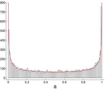
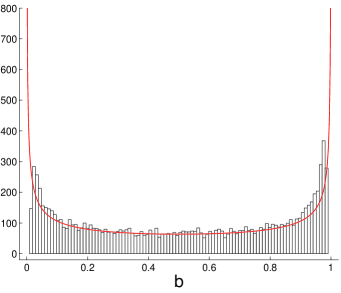
Figure 1:  Histograms for the occupation time functional $\eta_{T}^{+}(0;f)$ with (a) the Heaviside step function $f=H$ and (b) the function $f(x)=\pi^{\mbox{$\>\!$}-1}\mbox{$\;\!\!$}\arctan x+\frac{1}{2}$ . The parameters of the telegraph process $X_{t}^{+}$ are standardized to $c=1$ and $\lambda=1$. Both histograms are obtained with $N=10,\mbox{$\;\!\!$}000$ simulations, each over the observation time $T=1\mbox{$\;\!$}000$. The length of each box on the histogram is $\Delta=0.01$. The red solid curve represents the scaled arcsine density (i.e., multiplied by $N\Delta=100$).

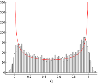
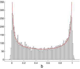
Figure 2:  Histograms for the functional $\eta_{T}^{+}(0;f)$ with the probing function $f(x)=\pi^{\mbox{$\>\!$}-1}\mbox{$\>\!\!$}\arctan x+\cos x+\frac{1}{2}$ . The parameters of the telegraph process are as in Figure 1, with the same number of runs $N=10,\mbox{$\;\!\!$}000$ and the observation time (a) $T=1\mbox{$\;\!$}000$ or (b) $T=10\mbox{$\;\!$}000$. Compare with Figure 1 and note the improved quality of fit to the hypothetical arcsine distribution (red curve) on the right plot as compared to the left one.

The long-term prediction contained in a more general Theorem 2.4 was verified by computer simulations for the functional $\eta_{T}^{+}(0;f)$ with the probing function $f(x)=\pi^{-1}\mbox{$\>\!\!$}\arctan x+\frac{1}{2}$ . The new histogram plot (see Figure 1b), obtained with the same values of $c$, $\lambda$, $T$ and $N$, is qualitatively similar to that on Figure 1a, including a small right bias, but convergence to the arcsine distribution becomes slower, apparently due to additional time needed for the process to explore the limiting values $f_{\pm}$ of the function $f$ at $\pm\infty$, which eventually determine the distributional limit.

Incidentally, this observation helps to understand the difference between the sets of hypotheses in Theorems 2.3 and 2.4 ; indeed, the additional condition of Theorem 2.4, requiring that $c^{2}T\mbox{$\;\!\!$}/\lambda\to\infty$ as $T\to\infty$, guarantees a sufficient mobility of the telegraph process needed to gauge the limits $f_{\pm}$ available only at remote distances from the origin. In contrast, if the function $f$ is reduced to the Heaviside step function $H$, the limiting values $H_{-}\mbox{$\>\!\!$}=0$, $H_{+}\mbox{$\>\!\!$}=1$ are encountered by the process straight away, so no extra mobility is needed.

Let us point out that the asymptotic conditions imposed in Theorem 2.4 on the function $f$ involved in the occupation functional $\eta_{T}^{\pm}(x;f)$ are rather strong, assuming the existence of the limits $\lim_{x\to\pm\infty}f(x)=f_{\pm}$  (with $f_{-}\neq f_{+}$) . This is in contrast with the paper by Khasminskii [Kh99] mentioned in the Introduction, where the function $f$ is only assumed to be Cesàro $(C,1)$-summable, i.e., subject to a weaker condition $\lim_{x\to\pm\infty}\,x^{-1}\!\int_{0}^{x}f(u)\,{\rm d}{u}=f_{\pm}$  (cf. (1.4)). Unfortunately, we were unable to reach the same level of generality. In particular, our proofs of formulas (7.12), (7.14) and the key Lemmas 7.1 and 7.2 (see Section 7) are heavily based on the existence of the limits $f_{\pm}$.

However, we conjecture that Theorem 2.4 does hold under the weaker condition of Cesàro $(C,1)$-summability of the probing function $f$. To verify this claim numerically, we carried out computer simulations for the distribution of $\eta_{T}^{+}(0;f)$ with $f(x)=\pi^{\mbox{$\>\!$}-1}\mbox{$\>\!\!$}\arctan x+\cos x+\frac{1}{2}$ . Figure 2 a shows the simulated histogram with the old values $T=1\mbox{$\;\!$}000$ and $N=10,\mbox{$\;\!\!$}000$, which reveals a bimodal distribution but not quite well fit to the hypothetical arcsine limit; in particular, there are noticeable “parasite” shoulders outside the interval $[0,1]$, which are indeed possible because the function $f$ may take values less than $0$ and bigger than $1$. However, the fit with the arcsine shape significantly improves under longer observations, $T=10\mbox{$\;\!$}000$ (see Figure 2 b). In particular, the high modes at the edges are better pronounced, while the shoulders outside $[0,1]$ are considerably reduced.

Appendix A Probabilistic proof of Theorem 2.2

Let us recall some information related to the first-passage problem for the telegraph process $X^{\pm}_{t}$. For $x<0$, let $\mathfrak{T}^{\pm}_{-x}:=\min\{t\geq 0:X^{\pm}_{t}=-x\}$ (with the convention that $\inf\mbox{$\>\!$}\emptyset:=+\infty$) be the hitting time of point $-x>0$ by the process $X^{\pm}_{t}$ (starting from the origin, $X^{\pm}_{0}=0$). If we set $T_{0}:=(-x)/c$, then the distribution of $\mathfrak{T}_{-x}^{\pm}$ is concentrated on $[T_{0},\infty)$ and is given by (see [Pi91, § 0.5, pp. 12–13] and also [Or95, Theorem 4.1, p. 18])

$$\mathbb{P}\{\mathfrak{T}^{+}_{-x}\in{\rm d}{t}\}={\rm e}^{-\lambda T_{0}}\mbox{$\>\!$}\delta_{T_{0}}({\rm d}{t})+Q_{-x}^{+}(t)\,{\rm d}{t},\qquad\mathbb{P}\{\mathfrak{T}^{-}_{-x}\in{\rm d}{t}\}=Q_{-x}^{-}(t)\,{\rm d}{t},$$ (A.1)

where the densities $Q_{-x}^{\pm}$ are defined exactly by equations (2.13), (2.14).

Consider the two-dimensional Markov process $(X_{t}^{\pm},V_{t}^{\pm})$, where $X_{t}^{\pm}$ is the (conditional) telegraph process (1.6) (i.e., with the initial velocity $V_{0}=\pm c$, respectively), and $V_{t}^{\pm}={\rm d}X^{\pm}_{t}/{\rm d}{t}=\pm c\mbox{$\>\!$}(-1)^{N_{t}}$ is the corresponding velocity process driven by an dependent Poisson process $N_{t}$ which determines the reverse instants of the motion $X^{\pm}_{t}$ (see (1.6)). It is obvious that $\mathfrak{T}^{\pm}_{-x}$ is a stopping time for the process $(X^{\pm}_{t},V_{t}^{\pm})$. Also note that $V^{\pm}_{t}\bigr{|}_{t=\mathfrak{T}^{\pm}_{-x}}\!=+c$  (a.s), since the first passage through point $-x>0$ by the process $X^{\pm}_{t}$, starting from the origin, with probability $1$ can only occur from left to right, that is, with positive velocity. Hence, conditioning on the hitting time of the origin starting from $x<0$ (which, of course, has the same distribution as $\mathfrak{T}^{\pm}_{-x}$) and using the strong Markov property of the joint process $(X_{t}^{\pm},V_{t}^{\pm})$, we have, for each $y\in[0,1-T_{0}/T]$,

$$\mathbb{P}\{\mbox{$\>\!$}{} \eta_{T}^{\pm}(x)\in{\rm d}{y}\}=\mathbb{P}\{\mathfrak{T}^{\pm}_{-x}>T\}\mbox{$\>\!$}\delta_{0}({\rm d}{y})+\mathbb{E}\bigl{[}\mathbb{P}\{\eta^{\pm}_{T}(x)\in{\rm d}{y},\,T_{0}\leq\mathfrak{T}_{-x}^{\pm}\leq T\,|\,\mathfrak{T}_{-x}^{\pm}\}\bigr{]}$$

$$=\left(\int_{T}^{\infty}\mathbb{P}\{\mathfrak{T}^{\pm}_{-x}\in{\rm d}{u}\}\right)\delta_{0}({\rm d}{y})+\int_{T_{0}}^{(1-y)\mbox{$\>\!$}T}\mathbb{P}\{\mathfrak{T}^{\pm}_{-x}\in{\rm d}{u}\}\,\mathbb{P}\{(1-u/T)\,\eta^{+}_{T-u}(0)\in{\rm d}{y}\}.$$ (A.2)

Here, the first integral represents the case where the telegraph process $X^{\pm}_{t}$ does not reach the origin before time $T$ and, therefore, never enters the positive half-line (thus contributing to the atom $\delta_{0}({\rm d}{y})$), while the second integral (where integration is taken with respect to ${\rm d}{u}$) accounts for the first passage event (at time instant $u\in[T_{0},(1-y)T]$), so that the telegraph process, restarted from the origin (with the initial velocity $+c$), has to spend on the positive half-line the required time $T\mbox{$\>\!$}{\rm d}{y}$ during the remaining travel time $T-u$.

In view of (A.1) together with (2.13) and (2.14), and due to equation (2.8) which provides the distribution of $\eta_{T-u}^{+}(0)$, formula (A.2) furnishes an explicit representation of the distribution of $\eta_{T}^{\pm}(x)$. More explicitly, on account of the atom in (A.1), the right-hand side of (A.2) specializes to

$$\left(\int_{T}^{\infty}Q^{\pm}_{-x}(u)\,{\rm d}{u}\right)\delta_{0}({\rm d}{y})+\mu^{\pm}_{T}({\rm d}{y})+\int_{T_{0}}^{(1-y)\mbox{$\>\!$}T}\!Q^{\pm}_{-x}(u)\;\mathbb{P}\left\{\eta^{+}_{T-u}(0)\in\frac{{\rm d}{y}}{1-u/T}\right\}{\rm d}{u}\mbox{$\>\!$},$$ (A.3)

where $\mu^{-}_{T}({\rm d}{y}):=0$ and

$$\mu_{T}^{+}({\rm d}{y}):={\rm e}^{-\lambda T_{0}}\,\mathbb{P}\left\{\eta^{+}_{T-T_{0}}(0)\in\frac{{\rm d}{y}}{1-T_{0}/T}\right\}.$$ (A.4)

Using (2.8), for any $u\in[T_{0},(1-y)\mbox{$\>\!$}T]$ we have

$$\mathbb{P}\left\{\eta^{+}_{T-u}(0)\in\frac{{\rm d}{y}}{1-u/T}\right\}=2\varphi_{T-u}(1)\,\delta_{1-u/T}({\rm d}{y})+\psi_{T-u}\left(\frac{y}{1-u/T}\right)\frac{{\rm d}{y}}{1-u/T}\,.$$ (A.5)

Substituting (A.5) (with $u=T_{0}$) into (A.4) readily gives (2.11), while the last term on the right-hand side of (A.3) is reduced to (cf. (2.10))

$$2\mbox{$\>\!$}T\mbox{$\>\!$}Q^{\pm}_{-x}((1-y)T)\,\varphi_{T}(y)\,{\rm d}{y}+\int_{T_{0}}^{(1-y)\mbox{$\>\!$}T}Q^{\pm}_{-x}(u)\left(\psi_{T-u}\left(\frac{y}{1-u/T}\right)\frac{{\rm d}{y}}{1-u/T}\right){\rm d}{u}\mbox{$\>\!$},$$

where the contribution of the atom $\delta_{1-u/T}({\rm d}{y})$ from (A.5) is easily computed via the obvious symbolic formula $\delta_{1-u/T}({\rm d}{y})\,{\rm d}{u}=T\delta_{(1-y)T}({\rm d}{u})\,{\rm d}{y}$ . Indeed, for any test functions $F(y)$ and $G(u)$ we have, by changing the order of integration,

$$\int_{0}^{1-T_{0}/T}\!F(y) \int_{T_{0}}^{(1-y)\mbox{$\>\!$}T}\!G(u)\,\delta_{1-u/T}({\rm d}{y})\,{\rm d}{u}=\int_{T_{0}}^{T}G(u)\,{\rm d}{u}\int_{0}^{1-u/T}F(y)\,\delta_{1-u/T}({\rm d}{y})$$

$$=\int_{T_{0}}^{T}G(u)\,F(1-u/T)\,{\rm d}{u}=T\int_{0}^{1-T_{0}/T}F(y)\left(\int_{T_{0}}^{(1-y)T}G(u)\,\delta_{(1-y)\mbox{$\>\!$}T}({\rm d}{u})\right){\rm d}{y}\mbox{$\>\!$}.$$

Appendix B Probabilistic proof of Theorem 2.3

Making the substitution $t=Tu$ and using that $H(\alpha x)\equiv H(x)$ for any $\alpha>0$, we can rewrite formula (2.1) as

$$\eta_{T}^{\pm}(x)=\int_{0}^{1}H(x+X^{\pm}_{Tu})\,{\rm d}{u}=\int_{0}^{1}H(\tilde{x}+\tilde{X}^{\pm}_{u})\,{\rm d}{u},$$ (B.1)

where $\tilde{x}:=(c^{2}T/\lambda)^{-1/2}x$, and $\tilde{X}_{u}^{\pm}:=(c^{2}T/\lambda)^{-1/2}X_{Tu}^{\pm}$ ($u\geq 0$) is another telegraph process with rescaled parameters $\tilde{\lambda}:=\lambda T\to\infty$,  $\tilde{c}:=(\lambda T)^{1/2}\to\infty$  ($T\to\infty$). By Theorem 1.1, the process $(\tilde{X}_{u}^{\pm},\,0\leq u\leq 1)$ converges weakly to a standard Brownian motion $(B_{u},\,0\leq u\leq 1)$. Hence, if $\tilde{x}\to a$ as $T\to\infty$ (cf. the hypotheses of Theorem 2.3) then from (B.1) we immediately obtain the convergence in distribution, as $T\to\infty$,

$$\eta_{T}^{\pm}(x)\stackrel{{\scriptstyle\!d\,}}{{\to}}{\mathfrak{h}}_{1}(a):=\int_{0}^{1}H(a+B_{u})\,{\rm d}{u}.$$

According to (1.1) and (1.2), the random variable ${\mathfrak{h}}_{1}(0)$ has the arcsine distribution, which proves Theorem 2.3 for $a=0$. For $a<0$ (so that $-a>0$), let $\tau_{-a}:=\min\{t\geq 0:B_{t}=-a\}$ be the hitting time of the point $-a$ by the Brownian motion $B_{t}$ starting from the origin ($B_{0}=0$). As is well known since P. Lévy’s paper [Le40, Théorème 2, p. 294] (see also [IM74, § 1.7, p. 26] or [Fe71, § VI.2 (e), pp. 174–175]), the random variable $\tau_{-a}$ has probability density $q_{-a}(\cdot)$ defined in (2.15). Note that $\tau_{-a}$ is a stopping time (with respect to the natural filtration $\mathcal{F}_{t}:=\sigma\{B_{s},\ 0\leq s\leq t\}$). Conditioning on $\tau_{-a}$ (when $a+B_{\tau_{-a}}=0$) and using the strong Markov property, we obtain, for any $y\in[0,1]$,

$$\mathbb{P}\{\mbox{$\>\!$}{}{\mathfrak{h}}_{1}(a)\in{\rm d}{y}\} =\mathbb{P}\{\tau_{-a}>1\}\,\delta_{0}({\rm d}{y})+\int_{0}^{1-y}q_{-a}(u)\;\mathbb{P}\{(1-u)\mbox{$\;\!$}{\mathfrak{h}}_{1-u}(0)\in{\rm d}{y}\}\,{\rm d}{u}$$

$$=\left(\int_{1}^{\infty}q_{-a}(u)\,{\rm d}{u}\right)\delta_{0}({\rm d}{y})+\left(\int_{0}^{1-y}\frac{q_{-a}(u)}{1-u}\,p_{\mathrm{as}}\!\left(\frac{y}{1-u}\right){\rm d}{u}\right){\rm d}{y},$$

which coincides with (2.17) (for $Y_{-a}$) in view of (2.18) and (2.19). Finally, the case $a>0$ easily follows by noting the obvious symmetry relation ${\mathfrak{h}}_{1}(a)\stackrel{{\scriptstyle d}}{{=}}1-{\mathfrak{h}}_{1}(-a)$ (cf. (2.3)).

References

• [AS72] A. Abramowitz and I. A. Stegun (eds.), Handbook of mathematical functions, with formulas, graphs, and mathematical tables, 9th printing (Dover, New York, 1972).
• [DMT08] R. C. Dalang, C. Mueller and R. Tribe, A Feynman-Kac-type formula for the deterministic and stochastic wave equations and other p.d.e.s, Trans. Amer. Math. Soc. 360 (2008), 4681–4703.
• [EKa47] P. Erdős and M. Kac, On the number of positive sums of independent random variables, Bull. Amer. Math. Soc. 53 (1947), 1011–1020.
• [EtK86] S. N. Ethier and T. G. Kurtz, Markov processes: Characterization and convergence, Wiley Series in Probability and Mathematical Statistics (Wiley, New York, 1986).
• [Fe71] W. Feller, An introduction to probability theory and its applications, vol. II, 2nd edn., Wiley Series in Probability and Mathematical Statistics (Wiley, New York, 1971).
• [Go51] S. Goldstein, On diffusion by discontinuous movements and on the telegraph equation, Quart. J. Mech. Appl. Math. 4 (1951), 129–156.
• [Ha99] K. P. Hadeler, Reaction transport systems in biological modelling, in: Mathematics inspired by biology, V. Capasso and O. Diekmann (eds.), Lecture Notes Math. 1714, 95–150 (Springer, Berlin, 1999).
• [HH05] T. Hillen and K. P. Hadeler, Hyperbolic systems and transport equations in mathematical biology, in: Analysis and numerics for conservation laws, G. Warnecke (ed.), 257–279 (Springer, Berlin, 2005).
• [HO00] T. Hillen and H. G. Othmer, The diffusion limit of transport equations derived from velocity-jump processes, SIAM J. Appl. Math. 61 (2000), 751–775.
• [IM74] K. Ito and H. P. McKean, Diffusion processes and their sample paths, 2nd corr. printing, Die Grundlehren der mathematischen Wissenschaften 125 (Springer, Berlin, 1974).
• [Ka74] M. Kac, A stochastic model related to the telegrapher’s equation, Rocky Mountain J. Math. 4 (1974), 497–509. Reprinted from: M. Kac, Some stochastic problems in physics and mathematics, Colloquium lectures in the pure and applied sciences, No. 2, hectographed, 102–122 (Field Research Laboratory, Socony Mobil Oil Company, Dallas, TX, 1956).
• [Kh99] R. Khasminskii, Arcsine law and one generalization, Acta Appl. Math. 58 (1999), 151–157.
• [Ko86] M. D. Kostin, Velocity of propagation in diffusional quantum theory, J. Statist. Phys.  45 (1986), 765–767.
• [Le40] P. Lévy, Sur certains processus stochastiques homogènes, Compositio Math. 7 (1940), 283–339.
• [OL01] A. Okuba and S. A. Levin, Diffusion and ecological problems: Modern perspectives, 2nd ed., Interdisciplinary Applied Mathematics 14 (Springer, Berlin, 2001).
• [Or90] E. Orsingher, Probability law, flow function, maximum distribution of wave-governed random motions and their connections with Kirchoff’s laws, Stochastic Process. Appl. 34 (1990), 49–66.
• [Or95] E. Orsingher, Motions with reflecting and absorbing barriers driven by the telegraph equation, Random Oper. Stochastic Equations 3 (1995), 9–21.
• [OH02] H. G. Othmer and T. Hillen, The diffusion limit of transport equations. II. Chemotaxis equations, SIAM J. Appl. Math. 62 (2002), 1222–1250.
• [Pi91] M. A. Pinsky, Lectures on random evolution (World Scientific, Singapore, 1991).
• [Ra97] N. E. Ratanov, Random walks in an inhomogeneous one-dimensional medium with reflecting and absorbing barriers, Theor. Math. Phys. 112 (1997), 857–865.
• [Ra99] N. Ratanov, Telegraph evolutions in inhomogeneous media, Markov Process. Related Fields 5 (1999), 53–68.
• [Ra06] N. Ratanov, Branching random motions, nonlinear hyperbolic systems and travelling waves, ESAIM Probab. Stat. 10 (2006), 236–257.
• [Ra07] N. Ratanov, A jump telegraph model for option pricing, Quant. Finance 7 (2007), 575–583.
• [RM08] N. Ratanov and A. Melnikov, On financial markets based on telegraph processes, Stochastics 80 (2008), 247–268.
• [St93] D. W. Stroock, Probability theory: An analytic view (Cambridge University Press, Cambridge, 1993).
• [Ta22] G. I. Taylor, Diffusion by continuous movements, Proc. London Math. Soc. (2) 20 (1922), 196–212.
• [Th54] W. Thomson, On the theory of the electric telegraph, Proc. Roy. Soc. Lond. 7 (1854), 382–399. Reprinted as Article LXXIII in: Mathematical and physical papers by Sir William Thomson, Vol. II, 61–76 (At The University Press, Cambridge, 1884), \urlhttp://www.archive.org/details/mathematicaland02kelvgoog (choose ‘Read Online’)
• [We55] A. G. Webster, Partial differential equations of mathematical physics, 2nd corr. ed. (Dover, New York, 1955).
• [We02] G. H. Weiss, Some applications of persistent random walks and the telegrapher’s equation, Physica A 311 (2002), 381–410.
• [Za04] S. Zacks, Generalized integrated telegraph processes and the distribution of related stopping times, J. Appl. Prob. 41 (2004), 497–507.