Abstract

A study of ray trajectories was undertaken for the Tamm medium which represents the spacetime of a cosmic spinning string, under the geometric-optics approximation. Our numerical studies revealed that: (i) rays never cross the string’s boundary; (ii) the Tamm medium supports evanescent waves in regions of phase space that correspond to those regions of the string’s spacetime which could support closed timelike curves; and (iii) a spinning string can be slightly visible while a non–spinning string is almost perfectly invisible.

Keywords: cosmic spinning string, Tamm medium, invisibility, metamaterial, ray tracing

1 Introduction

Parallels have been established between exotic optical phenomenons associated with certain metamaterials and those associated with curved spacetimes [1, 2, 3]. For example, negative-phase-velocity propagation of light — a notable property supported by certain negatively refracting metamaterials [4] — is associated with various spacetime metrics in a noncovariant formalism [5, 6, 7, 8, 9]. This parallelism is perhaps not surprising given that light propagation in vacuum subjected to a gravitational field is formally equivalent to light propagation in a nonhomogeneous bianisotropic medium — called a Tamm medium [10] — in flat spacetime [11, 12, 13]. The practical realization of Tamm mediums is edging ever closer due to rapid advances in the science of nanostructured materials, especially those relating to metamaterials supporting negative refraction or cloaking applications [14, 15].

The constitutive relations for the Tamm medium representing a spinning cosmic string were recently established [3]. Cosmic strings are topological defects associated with phase transitions which may represent traces of the very early universe, as is comprehensively described elsewhere [16, 17]. In the following sections we report on the trajectories of light rays in the Tamm medium representing the spacetime metric of a cosmic spinning string, in the geometric-optics regime. In particular, we report on a cloaking phenomenon — analogous to that associated with certain metamaterials [18] — which arises when the cosmic string’s angular momentum is set to zero, thereby rendering it almost perfectly invisible to optical probes.

2 Quasi–planewave analysis

We consider a cosmic spinning string that is aligned parallel to the $z$ axis. Let $\rho=\sqrt{x^{2}+y^{2}}$. The ‘ballpoint pen’ model [19] is adopted wherein the spacetime metric describing the string’s interior region $\rho<\rho_{s}$ is matched smoothly at $\rho=\rho_{s}$ to the spacetime metric describing the string’s exterior region $\rho>\rho_{s}$. The Tamm medium representing this cosmic spinning string is characterized by the constitutive relations [3]

$$\left.\begin{array}[]{l}\underline{D}(\underline{r},t)=\epsilon_{\scriptscriptstyle 0}\underline{\underline{\gamma}}(x,y)\mbox{ \tiny{${}^{\bullet}$} }\underline{E}(\underline{r},t)-\sqrt{\epsilon_{\scriptscriptstyle 0}\mu_{\scriptscriptstyle 0}}\;\underline{\Gamma}(x,y)\times\underline{H}(\underline{r},t)\vspace{4pt}\\ \underline{B}(\underline{r},t)=\mu_{\scriptscriptstyle 0}\underline{\underline{\gamma}}(x,y)\mbox{ \tiny{${}^{\bullet}$} }\underline{H}(\underline{r},t)+\sqrt{\epsilon_{\scriptscriptstyle 0}\mu_{\scriptscriptstyle 0}}\;\underline{\Gamma}(x,y)\times\underline{E}(\underline{r},t)\end{array}\right\}$$ (1)

in SI units. The scalar constants $\epsilon_{\scriptscriptstyle 0}$ and $\mu_{\scriptscriptstyle 0}$ denote the permittivity and permeability of vacuum in the absence of a gravitational field, while the 3$\times$3 dyadic

$$\underline{\underline{\gamma}}(x,y)=\frac{1}{\rho}\left(\begin{array}[]{ccc}\displaystyle{\frac{A^{2}x^{2}+\rho^{2}y^{2}}{A\rho^{2}}}&\displaystyle{\frac{\left(A^{2}-\rho^{2}\right)xy}{A\rho^{2}}}&0\\ \\ \displaystyle{\frac{\left(A^{2}-\rho^{2}\right)xy}{A\rho^{2}}}&\displaystyle{\frac{A^{2}y^{2}+\rho^{2}x^{2}}{A\rho^{2}}}&0\\ \\ 0&0&A\end{array}\right)$$ (2)

and the 3–vector

$$\underline{\Gamma}(x,y)=\frac{M}{\rho^{2}}\left(-y,\,x,\,0\right).$$ (3)

Herein the scalar quantities

$$A=\left\{\begin{array}[]{lr}\displaystyle{\frac{1}{\sqrt{\lambda}}\,\sin\left(\rho\sqrt{\lambda}\right),}&\rho\leq\rho_{s}\vspace{6pt}\\ \displaystyle{\cos\left(\rho_{s}\sqrt{\lambda}\right)\left[\rho+\rho_{s}\left(\frac{\tan\left(\rho_{s}\sqrt{\lambda}\right)}{\rho_{s}\sqrt{\lambda}}-1\right)\right],}&\rho>\rho_{s}\end{array}\right.$$ (4)

and

$$M=\left\{\begin{array}[]{lr}\displaystyle{2\alpha\left[\left(\rho-\rho_{s}\right)\cos\left(\rho\sqrt{\lambda}\right)-\frac{1}{\sqrt{\lambda}}\,\sin\left(\rho\sqrt{\lambda}\right)+\rho_{s}\right],}&\rho\leq\rho_{s}\vspace{6pt}\\ \displaystyle{2\alpha\left[-\frac{1}{\sqrt{\lambda}}\,\sin\left(\rho_{s}\sqrt{\lambda}\right)+\rho_{s}\right]}&\rho>\rho_{s}\end{array}\right.$$ (5)

are expressed in terms of the real–valued constants $\lambda$ and $\alpha$, which are related to the energy density and angular momentum respectively. As we discussed previously [3], the choice $\lambda=\left(\pi/\rho_{s}\right)^{2}$ ensures that the constitutive parameters of the Tamm medium coincide with those of vacuum (in flat spacetime) in the limits $\rho\to 0$ and $\infty$. In keeping with our earlier study [3], we set $\alpha=1$ for our numerical studies of a spinning string, and $\alpha=0$ for a non–spinning string.

Consistently with the geometric-optics approximation, we consider quasi–planewave electric and magnetic fields of the form [20]

$$\left.\begin{array}[]{l}\underline{E}(\underline{r},t)={\rm Re}\left\{\,\underline{E}_{\,\scriptscriptstyle 0}(\underline{r})\exp\left[i\left(k_{\scriptscriptstyle 0}\underline{k}\cdot\underline{r}-\omega t\right)\right]\right\}\vspace{6pt}\\ \underline{H}(\underline{r},t)={\rm Re}\left\{\,\underline{H}_{\,\scriptscriptstyle 0}(\underline{r})\exp\left[i\left(k_{\scriptscriptstyle 0}\underline{k}\cdot\underline{r}-\omega t\right)\right]\right\}\end{array}\right\},$$ (6)

where $\underline{E}_{\,\scriptscriptstyle 0}(\underline{r})$ and $\underline{H}_{\,\scriptscriptstyle 0}(\underline{r})$ are complex–valued amplitudes, $\omega$ is the angular frequency, and the vacuum wavenumber $k_{\scriptscriptstyle 0}=\omega\sqrt{\epsilon_{\scriptscriptstyle 0}\mu_{\scriptscriptstyle 0}}$. The relative wavevector $\underline{k}$ in the quasi–planewave representation (6) is a function of $\underline{r}$ but for later convenience we omit explicit reference to $\underline{r}$. Combining eqs. (1) and (6) with the source–free Maxwell curl postulates yields

$$\left[\nabla\left(\underline{k}\cdot\underline{r}\right)-\underline{\Gamma}(x,y)\right]\times\underline{E}_{\,\scriptscriptstyle 0}(\underline{r})-\sqrt{\frac{\mu_{\scriptscriptstyle 0}}{\epsilon_{\scriptscriptstyle 0}}}\,\underline{\underline{\gamma}}(x,y)\cdot\underline{H}_{\,\scriptscriptstyle 0}(\underline{r})=-\frac{1}{ik_{\scriptscriptstyle 0}}\,\nabla\times\underline{E}_{\,\scriptscriptstyle 0}(\underline{r}),$$ (7)

$$\left[\nabla\left(\underline{k}\cdot\underline{r}\right)-\underline{\Gamma}(x,y)\right]\times\underline{H}_{\,\scriptscriptstyle 0}(\underline{r})+\sqrt{\frac{\epsilon_{\scriptscriptstyle 0}}{\mu_{\scriptscriptstyle 0}}}\,\underline{\underline{\gamma}}(x,y)\cdot\underline{E}_{\,\scriptscriptstyle 0}(\underline{r})=-\frac{1}{ik_{\scriptscriptstyle 0}}\,\nabla\times\underline{H}_{\,\scriptscriptstyle 0}(\underline{r}).$$ (8)

In the geometric-optics regime, the constitutive parameters are assumed to vary very slowly over the distance of a wavelength. Accordingly, the right sides of eqs. (7) and (8) are set to zero, and $\nabla\left(\underline{k}\cdot\underline{r}\right)\approx\underline{k}$. Thus, eqs. (7) and (8) simplify to [21]

$$\left\{\left[\det\underline{\underline{\gamma}}(x,y)-\underline{p}\cdot\underline{\underline{\gamma}}(x,y)\cdot\underline{p}\,\right]\underline{\underline{I}}+\underline{p}\,\underline{p}\cdot\underline{\underline{\gamma}}(x,y)\right\}\cdot\underline{E}_{\,\scriptscriptstyle 0}(\underline{r})=\underline{0}\,,$$ (9)

where $\underline{p}=\underline{k}-\underline{\Gamma}(x,y)$ and $\underline{\underline{I}}$ denotes the identity 3$\times$3 dyadic. The dyadic enclosed in braces on the left side of eq. (9) is required to be nonsingular, in order for nontrivial solutions to exist. This leads to the dispersion relation [21]

$$\mathcal{H}\equiv\det\underline{\underline{\gamma}}(x,y)-\underline{p}\cdot\underline{\underline{\gamma}}(x,y)\cdot\underline{p}=0,$$ (10)

from which the magnitude $k$ of the relative wavevector $\underline{k}$ may be deduced. In fact, the $k$–roots of the dispersion relation (10) — corresponding to $\underline{k}=k$ $(\sin\theta\,\cos\phi,$ $\,\sin\theta\,\sin\phi,$ $\,\cos\theta)$ at $\underline{r}=\left(\rho\cos\sigma,\,\rho\sin\sigma,z\right)$ — may be expressed as

$$k=\frac{-b\pm\sqrt{b^{2}-4ac}}{2a},$$ (11)

where the coefficients

$$a = A^{2}\cos^{2}\theta+\left[A^{2}\cos^{2}\left(\sigma-\phi\right)+\rho^{2}\sin^{2}\left(\sigma-\phi\right)\right]\sin^{2}\theta,$$ (12)

$$b = 2M\rho\sin\theta\,\sin\left(\sigma-\phi\right),$$ (13)

$$c = M^{2}-A^{2}.$$ (14)

Although eq. (10) is a quadratic equation in $k$, it yields only one independent root, in consonance with vacuum being unirefringent [22].

In general, $k$ can be complex–valued with non–zero imaginary part. However, regimes where $\mbox{Im}\left\{k\right\}\neq 0$ correspond to evanescent waves and are therefore excluded from our study of ray trajectories. It is illuminating to characterize the phase space corresponding to $\mbox{Im}\left\{k\right\}\neq 0$. The discriminant term in eq. (11), namely,

$$b^{2}-4ac = 4\Big{(}M^{2}\rho^{2}\sin^{2}\theta\,\sin^{2}\left(\sigma-\phi\right)$$ (15)

$$-\left\{A^{2}\cos^{2}\theta+\left[A^{2}\cos^{2}\left(\sigma-\phi\right)+\rho^{2}\sin^{2}\left(\sigma-\phi\right)\right]\sin^{2}\theta\right\}\left(M^{2}-A^{2}\right)\Big{)},$$

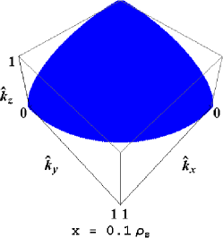
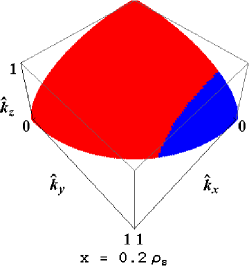
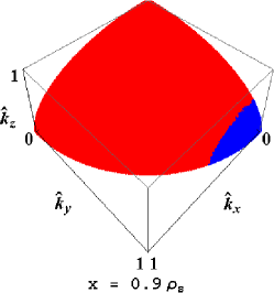
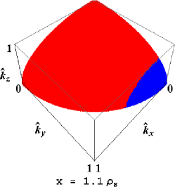
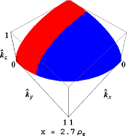
Figure 1: Maps illustrating the directions of $\underline{k}=k\left(\hat{k}_{x},\hat{k}_{y},\hat{k}_{z}\right)$ for which $\mbox{Im}\left\{k\right\}=0$ (blue) and $\mbox{Im}\left\{k\right\}\neq 0$ (red), at locations along the $x$ axis with $x\in\left\{0.1,0.2,0.9,1.1,2.7,3.0\right\}\rho_{s}$.

can only be negative–valued when $A^{2}-M^{2}<0$. Therefore, the regime where evanescent waves arise coincides exactly with the regime where the spacetime of a cosmic spinning string can support closed timelike curves [3, 23]. This regime is illustrated in Fig. 1, wherein the directions of $\underline{k}$ for which $\mbox{Im}\left\{k\right\}\neq 0$ are depicted at locations along the $x$ axis. For reasons of symmetry, only the directions in one octant of the unit sphere need be shown. We see that the $\mbox{Im}\left\{k\right\}\neq 0$ regime is restricted to the range $0.1<\left(\rho/\rho_{s}\right)<3$. Within this range, $\mbox{Im}\left\{k\right\}\neq 0$ for most $\underline{k}$ directions, but for $\underline{k}$ directed tangentially $k$ remains real–valued. It is clear from eq. (15) that for a non–spinning string (i.e., $M=0$), $k$ is real–valued for all $\underline{k}$ directions, at all locations.

3 Ray trajectories

The scalar quantity $\mathcal{H}$ introduced in eq. (10) serves as a convenient Hamiltonian function for our ray-tracing study. The ray trajectories are parameterized in terms of $\tau$ via $\underline{r}(\tau)$, and the relative wavevector is likewise parameterized as $\underline{k}(\tau)$. The coupled differential equations [24, 25]

$$\left.\begin{array}[]{l}\displaystyle{\frac{d\underline{r}}{d\tau}=\nabla_{\underline{k}}\mathcal{H}\vspace{10pt}}\\ \displaystyle{\frac{d\underline{k}}{d\tau}=-\nabla_{\underline{r}}\mathcal{H}}\end{array}\right\}$$ (16)

govern the trajectories of the light rays. Herein the shorthand $\nabla_{\underline{v}}\equiv\left(\partial/\partial v_{x},\,\partial/\partial v_{y},\,\partial/\partial v_{z}\right)$ for $\underline{v}=\left(v_{x},v_{y},v_{z}\right)$ is adopted.

Before proceeding, we confirm that the direction of a ray trajectory, i.e., $\nabla_{\underline{k}}\mathcal{H}$, coincides with the direction of energy flux. We know from earlier studies with a general Tamm medium that the time–averaged Poynting vector may be expressed as [26]

$$\langle\,\underline{P}\,\rangle_{t}=\beta\,\underline{\underline{\gamma}}(x,y)\cdot\underline{p}\,,$$ (17)

where the scalar $\beta$ is positive–valued provided that $\underline{\underline{\gamma}}(x,y)$ is either positive– or negative–definite. From eq. (2), the eigenvalues of $\underline{\underline{\gamma}}(x,y)$ are $\left\{A/\rho,A/\rho,\rho/A\right\}$; hence $\beta>0$. By direct vector differentiation of the definition of $\mathcal{H}$ provided in eq. (10), we find $\nabla_{\underline{k}}\mathcal{H}=2\,\underline{\underline{\gamma}}(x,y)\cdot\underline{p}$ . Therefore, the ray trajectories extracted from eqs. (16) are indeed parallel to the direction of energy flux.

Upon the specification of appropriate initial conditions $\underline{r}(0)$ and $\underline{k}(0)$, the system (16) can be solved for $\underline{r}(\tau)$ — and $\underline{k}(\tau)$ — by standard numerical methods, such as the Runge–Kutta method [25]. For a spinning string, two examples of ray trajectories are plotted in Fig. 2. In the first example, the rays start at locations in the $xy$ plane, with $\underline{k}(0)$ directed along $\left(-1,0,0\right)$. In this case the ray trajectories remain in the $xy$ plane. In the second example, $\underline{k}(0)$ is directed along $\left(-1,0,-1\right)$ and the ray trajectories are not restricted to one plane. In both examples, the ray trajectories skirt around the string’s boundary, never crossing it.

Let us now consider further whether it is possible for ray trajectories to cross the string’s boundary. In Fig. 3, trajectories are presented for rays which start close to the string boundary, at $\underline{r}(0)=\left(1.1,0,0\right)\rho_{s}$ and $\left(0.9,0,0\right)\rho_{s}$. Regardless of the direction of $\underline{k}(0)$, we find that rays which start outside the string’s boundary remain outside, and those which start inside the string’s boundary remain inside. We therefore conclude that rays cannot cross the string’s boundary, in either direction. Note that a ray starting right at the string’s boundary cannot be considered, as the geometric-optics approximation is not valid at this location.

4 Invisibility

The ray trajectories presented in Fig. 2 are reminiscent of those associated with metamaterials which are currently being investigated for cloaking applications [18, 27, 28, 29]. That is, the region inside the spinning string’s boundary is not visible to a distant observer. However, this self-cloaking cloaking effect is not perfect as the ray trajectories reaching a distant observer are distorted somewhat by the string.

In order to explore this matter further, let us consider a non–spinning string. The ray trajectories for a non–spinning string — corresponding to those presented in Fig. 2 for a spinning string — are presented in Fig. 4. We see that in a radial plane, the non–spinning string acts as an excellent cloak for itself: the interior of the string is hidden to a distant observer and there is minimal distortion to the ray trajectories reaching an observer more than a few radiuses away from the string. For rays traversing the string’s neighborhood at an oblique angle to the $z$ axis, there is a small degree of ray distortion close to the string — but this distortion diminishes as the distance from the string increases.

5 Closing remarks

The Tamm medium provides a convenient setting for simulating the passage of light through the spacetime associated with a cosmic spinning string. Based on a geometric-optics study, we have found that

• ray trajectories do not cross the string’s boundary; i.e., rays which start outside the string remain outside, whereas rays which start inside the string’s boundary remain trapped there;

• the regions of the spinning string’s spacetime which support closed timelike curves correspond to regions in the phase space of the Tamm medium which support evanescent waves; and

• a spinning string acts as an imperfect cloak for itself, while a non–spinning string cloaks itself almost perfectly.

These findings may well have far–reaching astronomical consequences, especially for those attempting to observe cosmic strings optically.

Acknowledgments: THA is supported by an EPSRC (UK) Vacation Bursary. TGM is supported by a Royal Academy of Engineering/Leverhulme Trust Senior Research Fellowship. AL thanks the Charles Godfrey Binder Endowment at Penn State for partial financial support of his research activities.

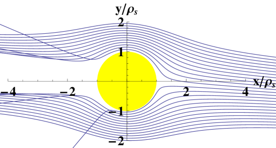
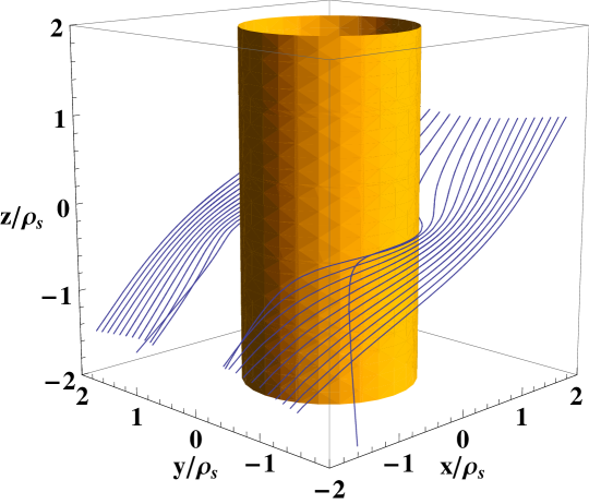
Figure 2: 2D and 3D examples of ray trajectories for a spinning string. Top: Rays start at equally spaced locations along the line $\underline{x}(0)=\left(40,\nu,0\right)\rho_{s}$ with $-3<\nu<-1$, and $\underline{k}(0)$ directed along $\left(-1,0,0\right)$. Bottom: Rays start at equally spaced locations along the line $\underline{x}(0)=\left(40,\nu,39\right)\rho_{s}$ with $-3.9<\nu<-1.9$, and $\underline{k}(0)$ directed along $\left(-1,0,-1\right)$.

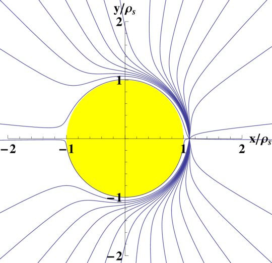
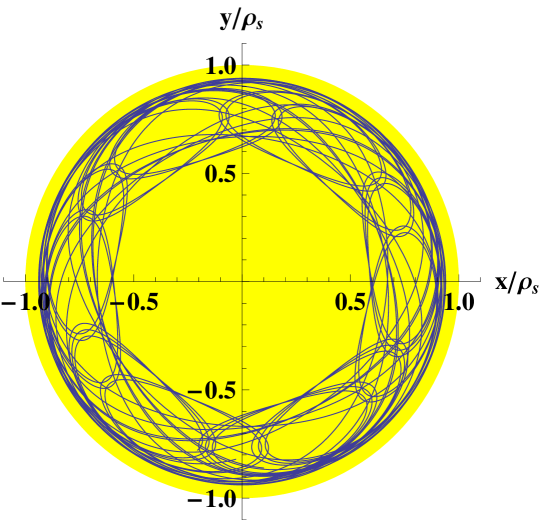
Figure 3: Examples of 2D ray trajectories that start at locations close to the spinning string’s boundary: $\underline{r}(0)=\left(1.1,0,0\right)\rho_{s}$ (top) and $\left(0.9,0,0\right)\rho_{s}$ (bottom). In both cases $\underline{k}(0)$ is oriented at equally spaced angular directions in the $xy$ plane. Note that for both locations approximately 70% of the possible orientations of $\underline{k}$ correspond to evanescent waves and are therefore not represented here.

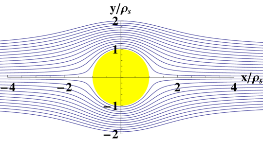
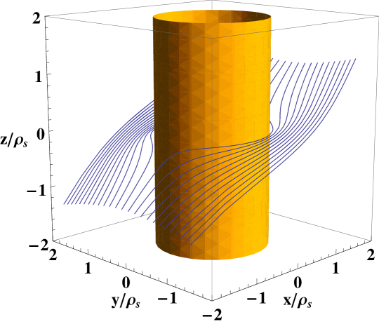
Figure 4: As Fig. 2 except that the string is not spinning and $-1<\nu<1$.

References

- [1] M. Li, R.–X. Miao, Y. Pang, Phys. Lett. B 689 (2010) 55.
- [2] Q. Cheng, T.J. Cui, W.X. Jiang, B.G. Cai, New J. Phys. 12 (2010) 063006.
- [3] T.G. Mackay, A. Lakhtakia, Phys. Lett. A 374 (2010) 2305.
- [4] T.G. Mackay, A. Lakhtakia, Phys. Rev. B 79 (2009) 235121.
- [5] T.G. Mackay, A. Lakhtakia, S. Setiawan, New J. Phys. 7 (2005) 171.
- [6] S.S. Komissarov, J. Kor. Phys. Soc. 54 (2009) 2503.
- [7] M. Sharif, U. Sheikh, J. Kor. Phys. Soc. 55 (2009) 1677.
- [8] B.M. Ross, T.G. Mackay, A. Lakhtakia, Optik 121 (2010) 401.
- [9] M. Hossain, M. Khayrul Hasan, Int. J. Theor. Phys. 48 (2009) 3007.
- [10] I.E. Tamm, Zhurnal Russkogo Fiziko-Khimicheskogo Obshchestva, Otdel Fizicheskii (J. Russ. Phys.-Chem. Soc., Phys. Section) 56 (1924) 248.
- [11] G.V. Skrotskii, Soviet Phys.–Dokl. 2 (1957) 226.
- [12] J. Plébanski, Phys. Rev. 118 (1960) 1396.
- [13] W. Schleich, M.O. Scully, in New Trends in Atomic Physics, eds. G. Grynberg, R. Stora (Elsevier Science Publishers, Amsterdam, Holland) 1984, p. 995.
- [14] U. Huebner, J. Petschulat, E. Pshenay-Severin, A. Chipouline, T. Pertsch, C. Rockstuhl, F. Lederer, Microelectron. Eng. 86 (2009) 1138.
- [15] P. He, J. Gao, Y. Chen, P. V. Parimi, C. Vittoria, V. G. Harris, J. Phys. D: Appl. Phys. 42 (2009) 155005.
- [16] M.B. Hindmarsh, T.W.B. Kibble, Rep. Prog. Phys. 58 (1995) 477.
- [17] A. Vilenkin, E.P.S. Shellard, Cosmological Strings and Other Topological Defects (Cambridge University Press, Cambridge, UK) 2000.
- [18] A. Greenleaf, Y. Kurylev, M. Lassas, G. Uhlmann, SIAM Rev. 51 (2009) 3.
- [19] B. Jensen, H.H. Soleng, Phys. Rev. D 45 (1992) 3528.
- [20] J. van Bladel Electromagnetic Fields (Hemisphere, Washington, DC, USA) 1985, pp. 269–274.
- [21] A. Lakhtakia, T.G. Mackay, J. Phys. A: Math. Gen. 37 (2004) L505. Erratum 37 (2004) 12093.
- [22] A. Lakhtakia, T.G. Mackay, Chin. Phys. Lett. 23 (2006) 832.
- [23] S. Slobodov, Found. Phys. 38 (2008) 1082.
- [24] M. Kline, I.W. Kay, Electromagnetic Theory and Geometric Optics (Interscience, New York, NY, USA) 1965, pp. 109–112.
- [25] M. Sluijter, D.K. de Boer, H.P. Urbach, J. Opt. Soc. Amer. A 26 (2009) 317.
- [26] T.G. Mackay, A. Lakhtakia, S. Setiawan, New J. Phys. 7 (2005) 75.
- [27] J. Shin, J.-T. Shen, S. Fan, Phys. Rev. Lett. 102 (2009) 093903.
- [28] R. Liu, C. Ji, J.J. Mock, J.Y. Chin, T.J. Cui, D.R. Smith, Science 323 (2009) 366.
- [29] H. Hashemi, B. Zhang, J.D. Joannopoulos, S.G. Johnson, Phys. Rev. Lett. 104 (2010) 253903.