A Selection Region Based Routing Protocol for Random Mobile ad hoc Networks

Abstract

We propose a selection region based multi-hop routing protocol for random mobile ad hoc networks, where the selection region is defined by two parameters: a reference distance and a selection angle. At each hop, a relay is chosen as the nearest node to the transmitter that is located within the selection region. By assuming that the relay nodes are randomly placed, we derive an upper bound for the optimum reference distance to maximize the expected density of progress and investigate the relationship between the optimum selection angle and the optimum reference distance. We also note that the optimized expected density of progress scales as $\Theta(\sqrt{\lambda})$, which matches the prior results in the literature. Compared with the spatial-reuse multi-hop protocol in [1] recently proposed by Baccelli et al., in our new protocol the amount of nodes involved and the calculation complexity for each relay selection are reduced significantly, which is attractive for energy-limited wireless ad hoc networks (e.g., wireless sensor networks).

I Introduction

In wireless ad hoc networks, each node may serve as the data source, destination, or relay at different time instants, which leads to a self-organized network. Such a decentralized structure makes the traditional network analysis methodology used in centralized wireless networks inadequate. In addition, it is hard to define and quantify the capacity of large wireless ad hoc networks. In the seminal work [2], Gupta and Kumar proved that the transport capacity for wireless ad hoc networks, defined as the bit-meters pumped every second over a unit area, scales as $\Theta(\sqrt{n})$ in an arbitrary network, where $n$ is node density. In [3], Weber et al. derived the upper and lower bounds on the transmission capacity of spread-spectrum wireless ad hoc networks, where the transmission capacity is defined as the product between the maximum density of successful transmissions and the corresponding data rate, under a constraint on the outage probability. However, the above work only considered single-hop transmissions.

In [4], with multi-hop transmissions and assuming all the transmissions are over the same transmission range, Sousa and Silvester derived the optimum transmission range to maximize a capacity metric, called the expected forward progress. Zorzi and Pupolin extended Sousa and Silvester’s work in [5] to consider Rayleigh fading and shadowing. Recently, Baccelli et al. [1] proposed a spatial-reuse based multi-hop routing protocol. In their protocol, at each hop, the transmitter selects the best relay so as to maximize the effective distance towards the destination and thus to maximize the spatial density of progress. By assuming each transmitter has a sufficient backlog of packets, Weber et al. in [6] proposed longest-edge based routing where each transmitter selects a relay that makes the transmission edge longest. In [7], Andrews et al. defined the random access transport capacity. By assuming that all hops bear the same distance with deterministically placed relays, they derived the optimum number of hops and an upper bound on the random access transport capacity.

Most of the above works with multi-hop transmissions (e.g., [4], [5], and [7]) assume that each hop traverses the same distance, which is not practical when nodes are randomly distributed. On the other hand, in [1] and [6] the authors proposed routing protocols with randomly distributed relays; but they did not address how to optimize the transmission distance at each hop. In this paper, by jointly considering the randomly distributed relays and the optimization for the hop distance, we propose a selection region based multi-hop routing protocol, where the selection region is defined by two parameters: a selection angle and a reference distance. By maximizing the expected density of progress, we derive the upper bound on the optimum reference distance and the relationship between the optimum reference distance and the optimum selection angle.

The rest of the paper is organized as follows. The system model and the routing protocol are described in Section II. The selection region optimization is presented in Section III. Numerical results and discussions are given in Section IV. The computational complexity is analyzed in Section V. Finally, Section VI summarizes our conclusions.

II System Model and Routing Protocol

In this section, we first define the network model, then present the selection region based routing protocol.

II-A Network Model

Assume nodes in the network follow a homogenous Poisson Point Process (PPP) with density $\lambda$, with slotted ALOHA being deployed as the medium access control (MAC) protocol. We also consider the nodes are mobile, to eliminate the spatial correlation, which is also discussed in [1]. During each time slot a node chooses to transmit data with probability $p$, and to receive data with probability $1-p$. Therefore, at a certain time instant, transmitters in the network follow a homogeneous PPP ($\Pi_{Tx}$) with density $p\lambda$, while receivers follow another homogenous PPP ($\Pi_{Rx}$) with density $(1-p)\lambda$. Considering multi-hop transmissions, at each hop a transmitter tries to find a receiver in $\Pi_{Rx}$ as the relay. We assume that all transmitters use the same transmission power $\rho$ and the wireless channel combines the large-scale path-loss and small-scale Rayleigh fading. The normalized channel power gain over distance $d$ is given by

$$G(d)=\frac{\gamma}{{{d^{\alpha}}}},$$ (1)

where $\gamma$ denotes the small-scale fading, drawn from an exponential distribution of mean $\frac{1}{\mu}$ with probability density function (PDF) $f_{\gamma}(x)=\mu\exp(-\mu x)$, and $\alpha>2$ is the path-loss exponent.

For the transmission from transmitter $i$ to receiver $j$, it is successful if the received signal-to-interference-plus-noise ratio (SINR) at receiver $j$ is above a threshold $\beta$. Thus the successful transmission probability over this hop with distance $d_{ij}$ is given by

$$P_{s}=\Pr\left(\frac{\rho\gamma_{0}d_{ij}^{-\alpha}}{\sum_{k\in\Pi_{TX}\setminus\{i\}}\rho\gamma_{i}{d_{kj}}^{-\alpha}+\eta}>\beta\right),$$ (2)

where $i\in\Pi_{Tx}$, $j\in\Pi_{Rx}$, $\sum_{k\in\Pi_{Tx}\setminus\{i\}}\rho\gamma_{i}{d_{kj}}^{-\alpha}$ is the sum interference from the simultaneous concurrent transmissions, $d_{kj}$ is the distance from interferer $k$ to receiver $j$, and $\eta$ is the average power of ambient thermal noise. In the sequel we approximate $\eta=0$, which is reasonable in interference-limited ad hoc networks. From [1], the successful transmission probability from transmitter $i$ to receiver $j$ is derived as

$$P_{s}=\exp\left(-\lambda{p}t{d_{ij}}^{2}\right),$$ (3)

where

$$t=\frac{{2{\pi^{2}}/\alpha}}{{\sin(2\pi/\alpha)}}{\beta^{2/\alpha}}.$$

II-B Selection Region Based Routing

Considering a typical multi-hop transmission scenario, where a data source (S) sends information to its final destination (D) that is located far away, and it is impossible to complete this operation over a single hop.

Since we assume that nodes are randomly distributed, relays may not be located at an optimum transmission distance as derived in [7]. To guarantee a relay existing at a proper position, we propose a selection region based multi-hop routing protocol. For each transmitter along the route to the final destination, we define a selection region by two parameters: a selection angle $\varphi$ and a reference distance $r_{m}$, as shown by the shaded area in Fig. 1, where the selection region is defined as the region that is located within angle $\varphi$ and outside the arc $\widehat{AB}$ with $|\overrightarrow{OB}|=r_{m}$. Here, the transmitter is placed in the circle center $O$, $\angle{BOC}=\angle{AOC}=\varphi/2$, and $\overrightarrow{OC}$ points to the direction of the final destination. At each hop, the relay is selected as the nearest receiver node to the transmitter among the nodes in the selection region.

The reason that we limit the selection region within an angle $\varphi$ is explained as follows: In multi-hop routing, a transmission is inefficient if the projection of transmission distance on the directional line from the transmitter towards the final destination is negative, or less efficient if the projection is positive but very small. Therefore, here we set a limiting angle $\phi$ with which each packet traverses at each hop within $[-\varphi/2,\varphi/2]$.

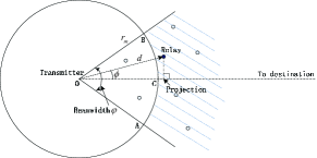
Figure 1: Selection region

Compared with the model in [7], where the authors assume that the relays are equidistantly placed along a line from the source to the destination as shown in Fig. 2, here our model assumes that the intermediate relays are randomly distributed over the selection region following a homogenous PPP ($\Pi_{Rx}$) with density $(1-p)\lambda$, which is more practical.

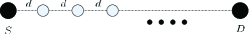
Figure 2: Ideal scenario: position-predetermined relays are equidistantly placed along the line from the source to the destination

III Selection Region Optimization

In this section, we optimize the selection region to derive the optimum values for the selection angle $\varphi$ and the reference distance $r_{m}$ by maximizing the expected density of progress.

As in [1], the density of progress is defined as

$$D=p\lambda\cdot P_{s}\cdot d\cos\phi,$$

where $P_{s}$ is the successful transmission probability defined in (2), $d\cos\phi$ is the projection of the transmission distance $d$ along the directional line $\overrightarrow{OC}$. Since the receivers follow a homogeneous PPP with density $\lambda(1-p)$, the cumulative distribution function (CDF) of the transmission distance $d$ is given as

$$\Pr(d\leq r)=1-\exp\left[-\lambda(1-p)\frac{\varphi}{2}({r^{2}}-r_{m}^{2})\right],{r_{m}}\leq r<\infty.$$ (3)

Since $\phi$ is uniformly distributed over $[-\varphi/2,\varphi/2]$, which is independent of $d$, the expected density of progress is given by

$$E[D] =p\lambda\int\limits_{r_{m}}^{\infty}\int\limits_{-\frac{\varphi}{2}}^{\frac{\varphi}{2}}{{e^{-p\lambda t{x^{2}}}}}x\cos\phi{f_{d}}(x)d\phi dx$$

$$=\sqrt{\lambda}p(1-p)\Gamma\left(\frac{3}{2},kr_{m}^{2}\right){k^{-3/2}}\exp\left(\lambda(1-p)\frac{\varphi}{2}r_{m}^{2}\right)\sin\left(\frac{\varphi}{2}\right),$$ (4)

where ${f_{d}}(x)$ is the PDF of $d$ obtained from (4), $k=pt+(1-p)\frac{\varphi}{2}$, $t$ is defined in (3a), and $\Gamma\left(\frac{3}{2},kr_{m}^{2}\right)=\int\limits_{kr_{m}^{2}}^{\infty}{{e^{-t}}{t^{\frac{3}{2}-1}}dt}$ is the incomplete Gamma function.

To optimize the objective function in (5), we first assume that $\varphi$ is constant, and try to derive the optimum value of $r_{m}$. For brevity, in the following derivation we write the objective function as $E$. Setting the derivative with respect to $r_{m}$ as 0, after some calculations we have

$$\frac{{dE}}{{dr_{m}}}= \exp\left(\lambda(1-p)\frac{\varphi}{2}r_{m}^{2}\right)$$

$$\cdot\left[\Gamma\left(\frac{3}{2},kr_{m}^{2}\right)\lambda(1-p)\varphi r_{m}+\frac{{d\Gamma\left(\frac{3}{2},kr_{m}^{2}\right)}}{{dr_{m}}}\right]=0,$$ (5)

where $\Gamma\left(\frac{3}{2},kr_{m}^{2}\right)$ is calculated as

$$\Gamma\left(\frac{3}{2},kr_{m}^{2}\right)=\Gamma\left(\frac{3}{2}\right)+\sqrt{k}{r_{m}}\exp\left(-kr_{m}^{2}\right)-\frac{{\sqrt{\pi}}}{2}erf\left(\sqrt{k}{r_{m}}\right).$$ (6)

Thus we have

$$\frac{{d\Gamma\left(\frac{3}{2},kr_{m}^{2}\right)}}{{dr_{m}}} =\sqrt{k}\exp\left(-kr_{m}^{2}\right)\left(1-2kr_{m}^{2}\right)-\sqrt{k}\exp\left(-kr_{m}^{2}\right)$$

$$=-2{k^{3/2}}r_{m}^{2}\exp\left(-kr_{m}^{2}\right).$$ (7)

Applying (8) to (6), we obtain

$$\Gamma\left(\frac{3}{2},kr_{m}^{2}\right)\lambda\left(1-p\right)\varphi{r_{m}}-2{k^{3/2}}r_{m}^{2}\exp\left(-kr_{m}^{2}\right)=0.$$ (8)

Note that the above is only the necessary condition for optimality, given the unknown convexity of objective function. However, the global optimum must be among all the roots of the above equation, which can be found numerically. Since it is difficult to analytically derive the exact solution for $r_{m}$ from (9), we turn to get an upper bound of $r_{m}$. Since

$$\Gamma\left(\frac{3}{2},kr_{m}^{2}\right) >\frac{1}{2}\left[\Gamma\left(1,kr_{m}^{2}\right)+\Gamma\left(2,kr_{m}^{2}\right)\right]$$

$$=\frac{1}{2}\exp\left(-kr_{m}^{2}\right)\left(2+kr_{m}^{2}\right),$$ (9)

by (9), we have

$$\lambda(1-p)k\varphi r_{m}^{2}-4{k^{3/2}}r_{m}+\lambda(1-p)\varphi>0.$$ (10)

Therefore,

$${r_{m}}<\frac{{2{k^{3/2}}-\sqrt{4{k^{3}}-2k{{[\lambda(1-p)\varphi]}^{2}}}}}{{k\lambda(1-p)\varphi}}.$$ (11)

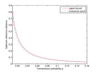
Figure 3: Numerical results and the analytical upper bound for the optimum reference distance

In Fig. 3, we compare the upper bound of the optimum $r_{m}$ with the numerically computed optimal value when $\varphi=\frac{1}{3}\pi$. We see that when transmission probability $p$ increases, the upper bound becomes tighter.

Now let’s maximize the objective function by jointly optimizing $r_{m}$ and $\varphi$. Rewrite (5) as

$$E=\sqrt{\lambda}p(1-p)\exp\left(-\lambda ptr_{m}^{2}\right)\Gamma\left(\frac{3}{2},kr_{m}^{2}\right)\exp\left(\lambda kr_{m}^{2}\right){k^{-3/2}}\sin\left(\frac{\varphi}{2}\right).$$

For brevity, let us denote $\exp(\lambda kr_{m}^{2})$ as $e$ and $\Gamma\left(\frac{3}{2},kr_{m}^{2}\right)$ as $\Gamma$. With partial derivatives, we have

$$\frac{{\partial E}}{{\partial r_{m}}}= \sqrt{\lambda}p(1-p)\sin\left(\frac{\varphi}{2}\right){k^{-3/2}}\exp\left(-\lambda ptr_{m}^{2}\right)$$

$$\cdot\left[-2\lambda pt{r_{m}}\Gamma e+\Gamma\frac{{\partial e}}{{\partial r_{m}}}+e\frac{{\partial\Gamma}}{{\partial r_{m}}}\right]=0.$$ (12)

This holds only if

$$\Gamma\frac{{\partial e}}{{\partial r_{m}}}+e\frac{{\partial\Gamma}}{{\partial r_{m}}}=2\lambda pt{r_{m}}\Gamma e.$$ (13)

Since $k=pt+(1-p)\frac{\varphi}{2}$, there is $\frac{{\partial k}}{{\partial\varphi}}=\frac{1}{2}(1-p)$. To simplify things, we can then calculate the derivative with respect to $k$ instead of $\varphi$ as

$$\frac{{\partial E}}{{\partial k}} =\sqrt{\lambda}p{(1-p)}\exp\left(-\lambda ptr_{m}^{2}\right)$$

$$\cdot\left[(\frac{{\cos(\varphi/2)}}{{1-p}}-\frac{3}{2}\sin\left(\frac{\varphi}{2}\right){k^{-1}})\Gamma e+\sin\left(\frac{\varphi}{2}\right)\left(\Gamma\frac{{\partial e}}{{\partial k}}+e\frac{{\partial\Gamma}}{{\partial k}}\right)\right]=0.$$ (14)

Since the factor in $e$ and $\Gamma$ related to $k$ and $r_{m}$ is only $kr_{m}^{2}$, thus we get $\frac{1}{2}r_{m}\frac{{\partial e}}{{\partial r_{m}}}=k\frac{{\partial e}}{{\partial k}}$ and $\frac{1}{2}r_{m}\frac{{\partial\Gamma}}{{\partial r_{m}}}=k\frac{{\partial\Gamma}}{{\partial k}}$.

Therefore, with (14), we have

$$\Gamma\frac{{\partial e}}{{\partial k}}+e\frac{{\partial\Gamma}}{{\partial k}}=\frac{{{r_{m}}}}{{2k}}\left(\Gamma\frac{{\partial e}}{{\partial{r_{m}}}}+e\frac{{\partial\Gamma}}{{\partial{r_{m}}}}\right)={k^{-1}}\lambda ptr_{m}^{2}\Gamma e.$$ (15)

Applying (16) to (15), the following holds:

$$\left[\frac{{\cos(\varphi/2)}}{{1-p}}-\frac{3}{2}\sin\left(\frac{\varphi}{2}\right){k^{-1}}\right]\Gamma e+\sin\left(\frac{\varphi}{2}\right){k^{-1}}\lambda ptr_{m}^{2}\Gamma e=0.$$ (16)

After some calculation, (17) is simplified as

$$\frac{{\cot(\varphi/2)k}}{{1-p}}-\frac{3}{2}+\lambda ptr_{m}^{2}=0.$$ (17)

Since it is hard to derive close-formed solutions for the optimal $r_{m}$ and $\varphi$, respectively, we implicitly use $\varphi$ and $p$ to express the optimal $r_{m}$ as

$$r_{m}=\sqrt{\frac{3/2-{\cot(\varphi/2)k/(1-p)}}{{\lambda pt}}}.$$ (18)

Note that $r_{m}$ scales as $\lambda^{-1/2}$, which intuitively makes sense. Since as the density increases, the interferers’ relative distance to the receiver decreases as $\sqrt{\lambda}$, it requires a shorter transmission distance by the same amount to keep the required SINR. By applying (19) in (5), we observe that (5) becomes $N\sqrt{\lambda}$, where $N$ is a constant independent of $\lambda$. This means that the maximum expected density of progress scales as $\Theta(\sqrt{\lambda})$, which conforms to the results in [2] and [7].

IV Numerical Results

In this section, we present some numerical results based on the analysis in Section III. We choose the path-loss exponent $\alpha$ as 3, the node density $\lambda$ as 1, and the outage threshold $\beta$ as 10 dB. In Figs. 4 and 5, we plot the expected density of progress vs. the reference distance $r_{m}$ and the selection angle $\varphi$, with $p=0.01$ and 0.05, respectively. We see that for each $p$ there exists an optimum selection angle and an optimum reference range when the respective partial derivatives are zero as discussed in Section III.

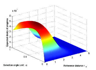
Figure 4: The expected density of progress vs. the reference distance and the selection angle with p=0.01

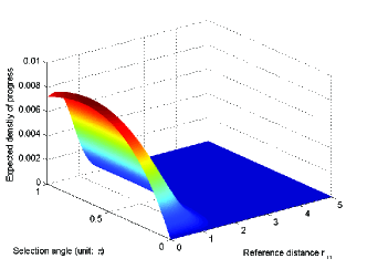
Figure 5: The expected density of progress vs. the reference distance and the selection angle with p=0.05

In Fig. 6, we plot the optimum selection angle obtained numerically vs. the transmission probability. As shown in the figure, we see that the increment of transmission probability leads to the increase of the optimum selection angle. This can be explained as follows: The increment of transmission probability means the decrement of the number of nodes that can be selected as relays; therefore the selection angle should be enlarged to extend the selection region.

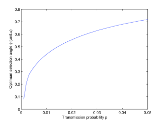
Figure 6: The optimum selection angle vs. the transmission probability p

In Fig. 7, we compare the optimum reference distance obtained numerically with that derived in (19), where $\varphi$ is chosen optimally as that in Fig. 6. We see that the increment of transmission probability leads to the decease of reference distance. This can be explained as follows: The increment of transmission probability means more simultaneous concurrent transmissions such that the interference will be increased; therefore the reference transmission distance should be decreased to guarantee the quality of the received signal and the probability of successful transmission.

In Fig. 8, we compare the performance of our routing protocol with that in [1], and also with the optimized (with optimum angle) nearest neighbor routing shown in Fig. 5 of [1] and the non-optimized (with an arbitrary angle, e.g., $\frac{\pi}{2}$) nearest neighbor routing in [8].

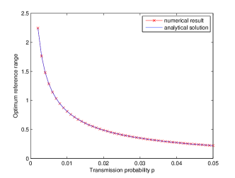
Figure 7: The optimum reference distance vs. the transmission probability p

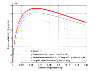
Figure 8: The performance of different routing protocols

From Fig. 8, we have the following observations and interpretations: 1)When $p$ increases, the performance of our routing protocol becomes close to that of the nearest neighbor routing with an optimum angle. This can be explained from Fig. 7 as: When $p$ increases, the reference distance $r_{m}$ tends to be a small value close to zero; thus our routing scheme degenerates to the nearest neighbor routing. Furthermore, our routing protocol shows much better performance than the non-optimized (with non-optimized angle) nearest neighbor routing, and this advantage is due to adopting both the optimum selection angle and the optimum reference distance. In this case, the selection region based routing can also be considered as the optimized nearest neighbor routing given the selection angle and the reference distance; 2) We see that when at the optimum selection angle and the optimum reference distance, the optimum transmission probability is approximately 0.05. Although in this paper we mainly focus on the optimization of the selection region, this observation indicates that there also exists an optimum transmission probability with our model, which has been discussed in some other prior literature, e.g., [1], [4], [5], and [6].

V Discussion on Complexity

As shown in Fig. 8, for multi-hop ad hoc networks, in terms of the performance metric of expected density of process, Baccelli et al.’s routing strategy is the best, by design at each hop the transmitter chooses a relay that provides the maximum value of progress towards the destination. However, the computational complexity with this protocol might be high, since the transmitter at each hop should compute the successful transmission probability $P_{s|x|}$ together with the projection of transmission distance, and accordingly evaluate the value of progress towards the destination for each receiver, further choose the one with the greatest value of progress as the relay.

In our protocol as we see from Fig. 8, when $p$ is small, its performance is close to that of Baccelli et al., while the computational complexity per hop is reduced significantly:

1) The nodes involved in the relay selection process are limited to a small region. As relays are selected from the receiver nodes in the selection region, the number of nodes participating in the relay selection is reduced with a ratio $\varphi/{2\pi}$ compared with that in [1].

2) Unlike that in [1], where the successful transmission probability $P_{s|x|}$, the projection of transmission distance, and further the value of progress towards the destination for each potential relay need to be calculated; we only need to calculate the distance between the transmitter and the potential relays.

Also note that our new protocol could be easily implemented by deploying directional antennas in the transmitter, where the spread angle can be set equal to the optimum selection angle. In this case not only the network computational complexity but also the interference will be reduced, which will be addressed in our future work.

VI Conclusions

In this paper, we propose a selection region based multi-hop routing protocol for random mobile ad hoc networks, where the selection region is defined by two parameters, a selection angle and a reference distance. By maximizing the expected density of progress, we present some analytical results on how to refine the selection region. Compared with the previous results in [4], [5], and [7], we consider the transmission direction at each hop towards the final destination to guarantee relay efficiency. Compared with the protocol in [1], the optimum selection region defined in this paper limits the area in which the relay is being selected, and the routing computational complexity at each hop is reduced.

References

- [1] F. Baccelli, B. Blaszczyszyn, and P. Muhlethaler, “An Aloha protocol for multihop mobile wireless networks,” IEEE Transactions on Information Theory, vol. 52, no. 2, pp. 421–436, Feb. 2006.
- [2] P. Gupta and P. R. Kumar, “The capacity of wireless networks,” IEEE Transactions on Information Theory, vol. 46, no. 2, pp. 388–404, Mar. 2000.
- [3] S. Weber, X. Yang, J. G. Andrews, and G. de Veciana, “Transmission capacity of wireless ad hoc networks with outage constraints,” IEEE Transactions on Information Theory, vol. 51, no. 12, pp. 4091–4102, Dec. 2005.
- [4] E.S. Sousa, and J.A. Silvester, “Optimum transmission ranges in a direct-sequence spread-spectrum multihop packet radio network,” IEEE Journal on Selected Areas in Communications, vol. 8, no. 5, pp. 762-771, Jun. 1990.
- [5] M. Zorzi, and S. Pupolin, “Optimum transmission ranges in multihop packet radio networks in the presence of fading,” IEEE Transactions on Communications, vol. 43, no. 7, pp. 2201-2205, Jul. 1995.
- [6] S. Weber, N. Jindal, R.K. Ganti, and M. Haenggi, “Longest Edge Routing on the Spatial Aloha Graph,” Proceedings of the IEEE GLOBECOM, pp. 1-5, Nov. 2008.
- [7] J. G. Andrews, S. Weber, M. Kountouris and M. Haenggi, “Random Access Transport Capacity,” IEEE Transactions On Wireless Communications, submitted. [Online] Available: http://arxiv.org/ps_cache/arxiv/pdf/0909/0909.5119v1.pdf.
- [8] M. Haenggi, “On routing in random Rayleigh fading networks,” IEEE Transactions on Wireless Communications, vol. 4, no. 4, pp. 1553-1562, Jul. 2005.