Phase Separation in Symmetric Mixtures of Oppositely Charged Rodlike Polyelectrolytes

Abstract

Phase separation in salt-free symmetric mixtures of oppositely charged rodlike polyelectrolytes is studied using quasi-analytical calculations. Stability analyses for the isotropic-isotropic and the isotropic-nematic phase transitions in the mixtures are carried out and demonstrate that electrostatic interactions favor nematic ordering. Coexistence curves for the symmetric mixtures are also constructed and are used to examine the effects of linear charge density and electrostatic interaction strength on rodlike polyelectrolyte complexation. It is found that the counterions are uniformly distributed in the coexisting phases for low electrostatic interaction strengths dictated by the linear charge density of the polyelectrolytes and Bjerrum’s length. However, the counterions also partition along with the rodlike polyelectrolytes with an increase in the electrostatic interaction strength. It is shown that the number density of the counterions is higher in the concentrated (or “coacervate”) phase than in the dilute (or supernatant) phase. In contrast to such rodlike mixtures, flexible polyelectrolyte mixtures can undergo only isotropic-isotropic phase separation. A comparison of the coexistence curves for weakly-charged rodlike mixtures with those of analogous flexible polyelectrolyte mixtures reveals that the electrostatic driving force for the isotropic-isotropic phase separation is stronger in the flexible mixtures.

I Introduction

For numerous biological processesdubin_review ; pe_complex_reviews ; vlad_muthu ; shklovskii_virus and emerging technologieswaite ; bazan_biosensor , complexation between oppositely charged polyelectrolytesvoorn_review ; veis_complexation ; kabanov_work1 ; kabanov_work2 ; dautzenberg_work1 ; pogodina_work ; dautzenberg_work2 is the underlying fundamental phenomenon. However, our understanding of how the electrostatic attraction between opposite charges on the polyelectrolytes is coupled with the conformational characteristics of polyelectrolyte chains is very limited. Motivated by a plethora of relevant biological processes and the impetus for developing advanced technologies such as underwater adhesiveswaite and biosensorsbazan_biosensor , extensive experimentaldubin_review ; pe_complex_reviews ; waite ; bazan_biosensor and theoreticalzhaoyang_complex ; voorn_review ; veis_complexation ; voorn_overbeek ; voorn_1 ; voorn_2 ; voorn_3 ; voorn_4 ; voorn_5 ; borue_complexation ; monica_complexation ; monica_complexation_2 ; joanny_01 ; jay_yuri_1 ; jay_yuri_2 work has been carried out to understand the mechanisms of polyelectrolyte charge complexation.

A few insights into the origin of polyelectrolyte complexation have been provided by simulations. Langevin dynamics simulationszhaoyang_complex of two oppositely charged polyelectrolyte chains have revealed that the entropy of counterion release is the predominant driving force for complexation in highly charged polyelectrolytes. In contrast, the simulations show that direct electrostatic attractions drive the association of two weakly charged polyelectrolytes whose counterions are not condensed onto the chains. Such simulations involving only a single pair of polymers are of course relevant only to extremely dilute solutions of polyelectrolytes and are only suggestive of complexation phenomena at finite concentrations. At such higher concentrations, complexation between oppositely charged polyelectrolytes has the character of a phase separation process in which a supernatant phase that is extremely dilute in polymer macroscopically separates from a polyelectrolyte rich phase that is either a fluid (“complex coacervate”) or a solid (“precipitate”). In this paper we shall be exclusively concerned with systems that produce fluid-like polyelectrolyte complexes properly classified as complex coacervates.dubin_review ; pe_complex_reviews ; voorn_review ; veis_complexation ; voorn_overbeek ; voorn_1 ; voorn_2 ; voorn_3 ; voorn_4 ; voorn_5 Extending conventional Langevin, Monte-Carlo, or molecular dynamics particle-based simulations to polyelectrolyte mixtures at finite concentrations has been hindered by the need for extremely large computational resources to address the long-range character of the electrostatic interactions and the inherently slow kinetics of the dense coacervate phase and phase separation process.

Development of a theory to study the phase separation in a mixture of oppositely charged polyelectrolytes is a daunting problem due to the non-trivial coupling between long range effects such as electrostatics and chain connectivity, and short range excluded volume interactions. The theoretical treatment is further complicated by the inevitable need to include electrostatic screening and correlation effects in the theory, analogous to the classical Debye-Hückel theory of electrolyte solutions, to capture the electrostatic forces that drive phase separation. This is the reason behind the inability of the self-consistent field theory (SCFT), a type of mean-field theory, to capture even the signature of a phase separationborue_complexation ; monica_complexation ; monica_complexation_2 ; joanny_01 ; jay_yuri_1 ; jay_yuri_2 . In other words, in a field-theoretic description of a mixed polyelectrolyte system, one needs to go beyond the mean-field or “saddle-point” approximation in order to study phase separation phenomena. Typically, the random phase approximationborue_complexation ; monica_complexation ; monica_complexation_2 is used to compute the leading correction to the saddle-point results. In the case of flexible polyelectrolytesmuthu_double , it can be shown rigorously that the random phase approximation is valid in the dual limit of high monomer densities and low small ion densities. Physically, such a situation is realized in concentrated solutions of weakly charged polyelectrolytes. More sophisticated field-theoretic results beyond the random phase approximation have also been obtained (including a phase diagram) for a particular model of flexible polyelectrolyte mixtures using the self-consistent one-loop (Hartree) approximationjoanny_01 . Most recently, direct numerical simulations of a related field theory model (so-called “field-theoretic simulations”) have been carried outjay_yuri_1 ; jay_yuri_2 to capture the effects of fluctuations and correlations to all orders, without invoking any approximation. An important result that came out of these simulations of flexible polyelectrolyte mixtures is that the phase boundaries in the concentrated regime are accurately predicted by the random phase approximation.

In this work, we consider solutions containing binary mixtures of oppositely charged rodlike polyelectrolytes and study their phase behavior using the random phase approximation, which, as noted above, has been previously shown to provide an accurate description of complexation phenomena in flexible polyelectrolyte mixtures. An important focus of our study is a comparison of the phase behavior of rodlike and flexible polyelectrolyte mixtures. The rodlike system is particularly relevant to a recently developed biosensor technologybazan_biosensor involving complexation of cationic conjugated polyelectrolytes with anionic DNA.

A fundamental question that we have tried to answer is: what is the role played by the flexibility of the polyelectrolytes in the phase separation processes that lead to a complex coacervate? Unlike flexible polyelectrolyte mixturesborue_complexation ; monica_complexation ; monica_complexation_2 ; joanny_01 ; jay_yuri_1 ; jay_yuri_2 , local enhancements in concentration of rodlike systems can produce orientationally ordered liquid crystalline phases (such as nematic, smectic and cholesteric phases).degennes_prost Thus, a coacervate produced by complexing oppositely charged rodlike polymers may be a liquid crystal rather than an isotropic fluid. In this paper, where we consider “symmetric” achiral rodlike polymers with fore-aft symmetry, equal length, and equal but opposite charge, we have explored the competition between isotropic and nematic ordering in rodlike polyelectrolyte mixtures and elucidated how the phase boundaries depend on different parameters of the system.

Before presenting our theory and numerical results on the binary mixtures, it is worthwhile to briefly review the theoretical literature aimed at understanding the phase separation of single component flexibledegennes_pincus ; joanny_leibler ; khokhlov_nyrkova ; muthu_weak_polymer ; chilun_muthu and rodlikeonsager_paper ; odijk_pe_rods ; chen_koch ; carri_muthu99 ; potemkin_1 ; potemkin_2 ; potemkin_3 ; stell_rods polyelectrolyte solutions. These studies have been primarily focused on poor solvent conditions. In the case of solutions containing a flexible polyelectrolyte, it has been shown that the dependence of the phase boundaries on the polyelectrolyte chain length is weak (referred to as the “weak polymer effect”muthu_weak_polymer ). Note that the condition of Donnan equilibrium was invoked in these calculations so that locally the system is electroneutral. This implies that a local increase in the charge on the polyelectrolyte leads to an increase in the local concentration of counterions. The localisation of the counterions is entropically unfavorable and hence, the region of two-phase coexistence shrinks with an increase in the charge on the polyelectrolyte chainsjoanny_leibler ; khokhlov_nyrkova ; muthu_weak_polymer .

Phase-separating mixtures of two oppositely charged polyelectrolytes are fundamentally different from these solutions containing a single kind of polyelectrolyte in two ways. Firstly, oppositely charged polyelectrolyte mixtures can phase separate even under good solvent conditions for the two individual polymer components. Secondly, it is clear in the binary mixture case that counterions are free to partition very differently upon phase separation. In particular, Donnan equilibrium can be satisfied by bringing the oppositely charged macromolecules together in the concentrated coacervate phase,voorn_1 ; voorn_2 ; voorn_3 ; voorn_4 ; voorn_5 while freeing the small ions to gain entropy by populating both dilute and concentrated phase in charge compensating proportions. Clearly, it is necessary to account for these extra degrees of freedom available to the counterions in studying phase separation in mixtures of oppositely charged polyelectrolytes.

In the case of single component rodlike polyelectrolyte solutions, it has been shown recentlypotemkin_1 ; potemkin_2 ; potemkin_3 that electrostatic interactions among like-charged rods favors orientational ordering at concentrations lower than the overlap concentration. This non-trivial result is an outcome of long-range, multi-rod correlations present in these systems. A consequence is that, in addition to the lyotropic isotropic-nematic transition observed in neutral rodlike solutions, thermotropic isotropic-nematic as well as nematic-nematic phase transitions have been predicted for charged rodlike polyelectrolytes. Note that these predictions are a consequence of collective phenomena at higher concentrations that are not manifest in earlier theories of dilute rodlike polyelectrolytes, where the twisting effectonsager_paper ; parsegian of pairwise electrostatic interactions between rods was shown to destroy nematic orderingonsager_paper ; odijk_pe_rods ; chen_koch ; carri_muthu99 .

With this background on the phase separation in polyelectrolyte solutions, we present our theoretical model for the binary mixtures. This paper is organized as follows: the theory is presented in Section II, the results are presented in Section III, and Section IV contains our conclusions.

II Theory

We consider a symmetric binary mixture of rodlike polyelectrolytes bearing opposite charges on their backbone in the presence of the counterions originating from the polyelectrolyte chains. By symmetric mixtures, we mean mixtures containing equal number of polyelectrolyte chains, which are identical to each other in every aspect other than the sign of the charge they are bearing. For generality in the following, we maintain notation representing different polymeric species such as $n_{+}$ and $n_{-}$ representing the number of polycationic and polyanionic chains, resepectively. For the theoretical treatment, we consider a binary mixture of rods with the same diameters ($=d$) for each species but lengths $L_{k}$ for $k=+,-$. Furthermore, $\sigma_{k}$ is taken to be the linear charge density for polyelectrolytes of type $k=+,-$ so that there are $n_{ck}=\sigma_{k}L_{k}$ counterions released by each polyelectrolyte of type $k$. As the charge on the polymers is spread uniformly along their length, this description is often referred to as the “smeared charge” model. We specialize to the symmetric case only as needed after plugging $n_{+}=n_{-}=n,L_{+}=L_{-}=L$ and $\sigma_{+}=\sigma_{-}=\sigma$ at the appropriate place. Also, we work in the canonical ensemble with the volume of the system denoted by $\Omega$.

The solvent is treated implicitly and as a uniform dielectric background for the purpose of computing electrostatic interactions. The small ions are taken to be point like and we ignore short range structure, correlations, and polarization effects in the solvent.

II.1 Qualitative Picture and Scaling Analysis

Before presenting quantitative details of our theory for the symmetric rodlike polyelectrolyte mixtures, a qualitative picture can be drawn by using three important results available from the literature. First, the macrophase separation in the isotropic phase (by analogy with symmetric mixtures of flexible polylectrolytes) takes place at very low monomer densitiesborue_complexation ; monica_complexation ; monica_complexation_2 ; joanny_01 ; jay_yuri_1 ; jay_yuri_2 , when the electrostatic attractions between oppositely charged polyelectrolytes are strong enough to drive the phase separation. Second, the isotropic-nematic phase transition observed in neutral rodlike molecules and treated by Onsager and many othersedwardsbook ; degennes_prost ; onsager_paper ; flory_semiflex ; flory_rods ; khokhlov_semiflex ; khokhlov_semenov takes place at relatively high monomer densities above the overlap concentration and is driven primarily by entropic effects associated with the excluded volume of rodlike objects. Thirdly, we recall that addition of charges to rodlike polymers can induce thermotropic (temperature dependent) isotropic-nematic phase transitions, as opposed to the lyotropic (concentration dependent) transitions familiar in neutral rodlike polymer systems. The origin of this thermotropic behavior lies in the long-ranged electrostatic interactions, which depend on the charge on the polyelectrolytes and the temperature dependent Bjerrum’s length $l_{B}=e^{2}/(4\pi\epsilon_{0}\epsilon_{r}k_{B}T)$, which is the distance at which the Coulomb interaction energy between two elementary charges is of the order of thermal energy ($=k_{B}T,\;k_{B}$ being the Boltzmann’s constant and $T$ is the temperature). Here, $\epsilon_{0}$ and $\epsilon_{r}$ are the permittivities of vacuum and the medium, respectively.

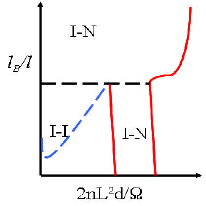
Figure 1: A qualitative sketch of the phase diagram in a symmetric mixture of oppositely charged rodlike polyelectrolytes. The symbols “I” and “N” denote regions of two-phase coexistence involving isotropic and nematic phases, respectively. $2n/\Omega,\;L$ and $d$ are the number density of positive and negative polyelectrolytes, the length, and the diameter of the charged rods, respectively. The y-axis is the ratio of the Bjerrum length $l_{B}$ to the monomer length $l$ and is a measure of electrostatic strength that is inversely proportional to temperature.

By integrating these three competing effects, a qualitative phase diagram of a symmetric rodlike polyelectrolyte mixture is sketched in Fig. 1 in the coordinates of $l_{B}/l$ versus $2nL^{2}d/\Omega$, where $l$ is a reference monomer length, $L$ is the overall rod length, $d$ is the rod diameter, $2n$ is the total number of cationic and anionic rods, and $\Omega$ is the system volume. Broadly, we see two trends in the figure. At high temperatures, i.e. low values of $l_{B}/l$, non-interacting isotropic-isotropic and isotropic-nematic coexistence regions appear at low and high rod concentrations, respectively. As the temperature is lowered ($l_{B}/l$ raised), these features collide and ultimately at low temperature there is a broad region of two phase coexistence between a dilute isotropic supernatant phase and a semidilute or concentrated nematic “coacervate” phase. At intermediate values of $l_{B}/l$, more complex phase behavior is evident, including the possibility of three-phase coexistence between two isotropic phases and a nematic phase.

With regard to the isotropic-isotropic coexistence region in Fig. 1, which is also present in flexible polyelectrolyte mixtures, a scaling analysis is helpful to understand the variables that control its extent and shape and differentiate the cases of rigid and flexible systems. For this purpose, we begin by considering a symmetric mixture containing an equal number $n$ of oppositely charged flexible polyelectrolytes in the absence of any counterions. Physically, such a situation is realized in a solution containing polyacids and polybases. Apart from electrostatic interactions, excluded volume effects can be simply accounted for (in an implicit solvent model) by an excluded volume parameter $w$. This particular system was recently studied using the field-theoretic simulation techniquejay_yuri_1 ; jay_yuri_2 . The osmotic pressure of such a system in the dilute regimedegennes_pincus ; rubinstein_review , i.e. $\rho=2nN/\Omega\ll\rho_{f}^{\star}\sim 1/(4\pi l_{B}\sigma^{2}N^{2})$, with $\rho,\;\rho_{f}^{\star}$ being the monomer density and the overlap concentration, respectively, is given by

$$\frac{P_{f}^{0}}{k_{B}T} = \frac{\rho}{N}+\frac{w}{2}\rho^{2}-\frac{\kappa_{d}^{3}}{24\pi},$$ (1)

where $\kappa_{d}^{2}=4\pi l_{B}\sigma^{2}N\rho$ is the Debye screening length in the asymptotic dilute regime where the polyelectrolytes behave as multivalent macroions. We note that although the polymers are assumed to be flexible, the expression that we use for $\rho_{f}^{\star}$ assumes that they adopt extended rodlike conformations at infinite dilution. In the above expression, $\sigma$ is the charge per monomer (in units of the fundamental charge $e$), which is the same for each kind of polyelectrolyte in the assumed symmetric mixture and $N$ is the total number of monomers.

In Eq.  1, the first and second terms correspond to the translational entropy of the polyelectrolyte chains and the effect of excluded volume interactions on the pressure, respectively. The third term containing $\kappa_{d}$, a Debye-Hückel contribution, originates from attractive electrostatic correlations among dilute, non-overlapping polyelectrolyte chains. In contrast, at higher polymer concentrations where chains overlap the internal structure of the polyelectrolytes plays a significant role. The dominant electrostatic contribution to the osmotic pressure in the high density, overlapping regime ($\rho\gg\rho_{f}^{\star}$) can be represented by the scaling expression

$$\frac{P_{f}^{e}}{k_{B}T} = -\frac{\kappa_{d}^{3}}{24\pi}\>\mathcal{F}\left(\rho/\rho_{f}^{\star}\right),$$ (2)

where $\mathcal{F}(x)$ is a dimensionless scaling function that we assume to be a power law $\sim x^{m}$ for large argument. The exponent $m$ is determined by the requirement that in the concentrated regime, the local properties are not different for a solution having multiple chains containing $N$ monomers each or a single chain that fills space with the same overall segment density $\rho$ ($N\rightarrow\infty$). In other words, the electrostatic contribution to the osmotic pressure must be independent of $N$ at fixed $\rho$, i.e. $P_{f}^{e}\sim N^{0}$. This requirement, along with the fact that the overlap concentration scales as $\rho_{f}^{\star}\sim 1/(4\pi l_{B}\sigma^{2}N^{2})$, leads to the well-known resultmuthu_double ; kaji_kanaya

$$\frac{P_{f}^{e}}{k_{B}T} \sim -\kappa_{p}^{3/2},$$ (3)

where $\kappa_{p}^{2}=4\pi l_{B}\sigma^{2}\rho$. In the concentrated regime, the osmotic pressure of flexible, symmetric polyelectrolyte mixtures is thus dictated by a balance between excluded volume and this modified electrostatic correlation energy, i.e.

$$\frac{P_{f}^{c}}{k_{B}T}\sim\frac{w}{2}\rho^{2}-\kappa_{p}^{3/2}$$ (4)

We can now retrace these scaling arguments for the case of symmetric mixtures of rodlike polylectrolytes. The osmotic pressure in the dilute concentration regime ($\rho\ll\rho_{r}^{\star}\sim 2nL^{2}d/\Omega$) is unchanged except that we replace the excluded volume coefficient $w$ with the Onsager expression $\pi dl^{2}/2$, where $l\equiv L/N$ is a monomer segment length,

$$\frac{P_{r}^{0}}{k_{B}T} = \frac{\rho}{N}+\frac{\pi dl^{2}}{4}\rho^{2}-\frac{\kappa_{d}^{3}}{24\pi}.$$ (5)

In the concentrated regime, the electrostatic free energy of a system of rods can be approximated by the sum of the self-energies of individual rods experiencing the electrostatic potential induced by the other rods. For the purpose of estimation, these are placed on a periodic lattice. It is well-known that the self-energy of a charged cylindrical rod of length $L$ and linear charge density $\sigma$ is divergentodijk_self ; safran_pincus , and is given by

$$\frac{U_{cyl}}{Lk_{B}T} \sim l_{B}\sigma^{2}\ln\frac{R}{\delta},$$ (6)

where $\delta$ is a cut-off introduced to regularize the self-energy and $R$ is the radius of a unit cell (Wigner-Seitz) applied to each cylinder. Using the fact that $R\sim 1/\sqrt{\rho}$ in the concentrated regime and writing the electrostatic free energy of the solution containing $n$ rods as $F^{e}=nU_{cyl}$, the electrostatic contribution to the pressure is given by

$$\frac{P_{r}^{e}}{k_{B}T} \sim -\kappa_{p}^{2}.$$ (7)

Comparing Eqs.  3 and  7, it is clear that the qualitative difference between flexible and rodlike polyelectrolyte mixtures is in the functional form for the attractive electrostatic contribution to the osmotic pressure. In the case of rodlike polyelectrolytes, this term scales like $\kappa_{p}^{2}\sim\rho$ in contrast to $\kappa_{p}^{3/2}\sim\rho^{3/4}$ for flexible coils. Thus, at the same set of electrostatic parameters and monomer densities, and for weakly charged polyelectrolytes where $\kappa_{p}\ll 1$, electrostatic correlation effects are weaker for rodlike polyelectrolytes in comparison with flexible polyelectrolyte mixtures. Since the electrostatic contribution to the pressure is responsible for polyelectrolyte complexation, it follows that rodlike polyelectrolyte mixtures are less prone to complex coacervation than analogous flexible polyelectrolyte mixtures. The regions of two-phase coexistence sketched in Fig. 1 should thus be narrower in rigid rod systems. This general observation will be born out by detailed numerical calculations in Section III of the spinodals and binodals of each type of system based on the free energy expression presented below.

II.2 Free Energy

An expression for the Helmholtz free energy of the assumed mixture of rodlike polyelectrolytes, counterions, and implicit solvent is derived in Appendix A using Onsager’s treatment for the neutral interactions and the random-phase approximation for the electrostatic interactions. Explicitly, the free energy is given by

$$F = F_{en}+F_{w}+F_{e}$$ (8)

where

$$\frac{F_{en}}{k_{B}T} = \sum_{j=+,-}n_{j}\int d\mathbf{u}_{j}\>p_{j}(\mathbf{u}_{j},\hat{\mathbf{n}})\ln\left[4\pi p_{j}(\mathbf{u}_{j},\hat{\mathbf{n}})\right]+\sum_{\gamma=+,-,c+,c-}n_{\gamma}\left[\ln\frac{n_{\gamma}}{\Omega}-1\right],$$ (9)

$$\frac{F_{w}}{k_{B}T} = \frac{1}{2\Omega}\sum_{j,k=+,-}^{\prime}n_{j}n_{k}\int d\mathbf{u}\int d\mathbf{u}^{\prime}\>p_{j}(\mathbf{u},\hat{\mathbf{n}})\left[2L_{j}L_{k}d|\mathbf{u}\times\mathbf{u}^{\prime}|\right]p_{k}(\mathbf{u}^{\prime},\hat{\mathbf{n}}),$$ (10)

$$\frac{F_{e}}{k_{B}T} = \frac{\Omega}{2}\int\frac{d^{3}\mathbf{q}}{(2\pi)^{3}}\left\{\ln\left[1+\frac{\kappa^{2}+\sum_{k=+,-}\kappa_{k}^{2}t_{k}(qL_{k})}{q^{2}}\right]-\frac{\kappa^{2}+\sum_{k=+,-}\kappa_{k}^{2}t_{k}(qL_{k})}{q^{2}}\right\}$$ (11)

and

$$t_{k}(qL_{k}) = \int d\mathbf{u}\>p_{k}(\mathbf{u},\hat{\mathbf{n}})\left[\frac{\sin\left[\left(\mathbf{q}\cdot\mathbf{u}\right)L_{k}/2\right]}{\left[\left(\mathbf{q}\cdot\mathbf{u}\right)L_{k}/2\right]}\right]^{2},\quad\mbox{for}\quad k=+,-.$$ (12)

Here, $\kappa$ is the inverse of the Debye screening length for small ions given by $\kappa^{2}=4\pi l_{B}\sum_{\gamma=c+,c-}Z_{\gamma}^{2}n_{\gamma}/\Omega$ so that $Z_{\gamma}$ is the valency (with sign) of the charged species of type $\gamma$. We define a similar object for the two polymer species: $\kappa_{k}^{2}=4\pi l_{B}Z_{k}^{2}\sigma_{k}^{2}L_{k}^{2}n_{k}/\Omega,Z_{k}$ being the valency of the charged monomers of type $k$. The functions $p_{k}(\mathbf{u},\hat{\mathbf{n}})$ represent the probability distribution function for finding a rod of type $k$ oriented along the unit vector $\mathbf{u}$ when the director is chosen to be the unit vector $\hat{\mathbf{n}}$. Each distribution function satisfies the normalization condition $\int d\mathbf{u}\>p_{k}(\mathbf{u},\hat{\mathbf{n}})=1$. Finally, the primed superscript in the expression for $F_{w}$ indicates that the $j=k$ terms are omitted from the double sum.

So far, the theory is quite general and the subsequent analysis depends on the functional form for the orientational probability distribution function for the rods. In this work, we focus on possibilities for phase separation that involve the isotropic and nematic phases only. For these two phases, $p_{k}(\mathbf{u},\hat{\mathbf{n}})\equiv p_{k}(\mathbf{u}\cdot\hat{\mathbf{n}})$ and the free energy for the each phase can be evaluated as described below.

II.3 Isotropic Phase

We begin by considering the isotropic phase, in which case the orientation distribution function for the rods is independent of the angle between the director $\hat{\mathbf{n}}$ and the unit vector along the axes of the rods ($\mathbf{u}$). In this case, $p_{k}(\mathbf{u}\cdot\hat{\mathbf{n}})=1/4\pi$ (obtained from the normalization condition) for $k=+,-$ so that the free energy in Eq.  8 can be written as

$$F^{iso} = F_{en}^{iso}+F_{w}^{iso}+F_{e}^{iso}$$ (13)

where

$$\frac{F_{en}^{iso}}{k_{B}T} = \sum_{\gamma=+,-,c+,c-}n_{\gamma}\left[\ln\frac{n_{\gamma}}{\Omega}-1\right],$$ (14)

$$\frac{F_{w}^{iso}}{k_{B}T} = \frac{\pi d}{4\Omega}(n_{+}L_{+}+n_{-}L_{-})^{2},$$ (15)

$$\frac{F_{e}^{iso}}{k_{B}T} = \frac{\Omega}{2}\int\frac{d^{3}\mathbf{q}}{(2\pi)^{3}}\left\{\ln\left[1+\frac{\kappa^{2}+\sum_{k=+,-}\kappa_{k}^{2}t^{iso}(qL_{k})}{q^{2}}\right]-\frac{\kappa^{2}+\sum_{k=+,-}\kappa_{k}^{2}t^{iso}(qL_{k})}{q^{2}}\right\}$$ (16)

and

$$t^{iso}(qL_{k}) = \frac{2Si(qL_{k})}{qL_{k}}-\left(\frac{2\sin\left(qL_{k}/2\right)}{qL_{k}}\right)^{2},$$ (17)

where $Si(x)=\int_{0}^{x}dt\frac{\sin t}{t}$ is the sine integral.

In the following, we rigorously show that the scaling argument presented in section  II.1 predicting a logarithmic correction to the free energy of isotropic phase in the mixtures of rods is indeed correct. For the analysis, we use the following asymptotic expressions for $t^{iso}(qL_{k})$ :

$$t^{iso}(qL_{k})=\left\{\begin{array}[]{ll}1,&qL_{k}\rightarrow 0\\ \pi/qL_{k},&qL_{k}\rightarrow\infty.\end{array}\right.$$ (18)

Also, we consider two limiting cases of short and long rods. For these cases, the electrostatic contribution to the free energy depends on how these limits are being approached. These limits can be approached by either fixing the linear charge density or the net charge per rod during the variation of length $L_{k}$. In the former case, $\kappa_{k}$ increases (decreases) with an increase (decrease) in $L_{k}$ and diverges (vanishes) strictly in the limit of $L_{k}\rightarrow\infty$ ($L_{k}\rightarrow 0$). On the other hand, for the latter approach, $\kappa_{k}$ is held fixed, while approaching the limits of $L_{k}\rightarrow\infty$ or $L_{k}\rightarrow 0$. Consider the latter case so that $\kappa_{k}$ is well-defined in approaching either limits of $L_{k}$.

Defining a Debye-like parameter proportional to the total ionic strength, $\kappa_{eff}^{2}=\kappa^{2}+\sum_{k=+,-}\kappa_{k}^{2}$ and approaching the limit of short rods, $L_{k}\rightarrow 0$ while keeping the charge per rod fixed, the free energy becomes

$$\frac{F^{iso}\left\{L_{k}\rightarrow 0\right\}}{k_{B}T} = \sum_{\gamma=+,-,c+,c-}n_{\gamma}\left[\ln\frac{n_{\gamma}}{\Omega}-1\right]+\frac{\pi d}{4\Omega}(n_{+}L_{+}+n_{-}L_{-})^{2}-\frac{\Omega\kappa_{eff}^{3}}{12\pi}.$$ (19)

Similarly, consider the limit of long rods, i.e. $L_{k}$ being large and approaching $\infty$. Approaching this limit while keeping the charge per rod fixed, the free energy becomes

$$\frac{F^{iso}\left\{L_{k}\rightarrow\infty\right\}}{k_{B}T} = \sum_{\gamma=+,-,c+,c-}n_{\gamma}\left[\ln\frac{n_{\gamma}}{\Omega}-1\right]+\frac{\pi d}{4\Omega}(n_{+}L_{+}+n_{-}L_{-})^{2}+\frac{F_{e}^{iso}\left\{L_{k}\rightarrow\infty\right\}}{k_{B}T},$$

where the electrostatic contribution to the free energy is given by

$$\frac{F_{e}^{iso}\left\{L_{k}\rightarrow\infty\right\}}{k_{B}T} = \frac{\Omega}{2}\int\frac{d^{3}\mathbf{q}}{(2\pi)^{3}}\left\{\ln\left[1+\frac{\kappa^{2}}{q^{2}}+\frac{\pi\kappa_{p}^{2}}{q^{3}}\right]-\frac{\kappa^{2}}{q^{2}}-\frac{\pi\kappa_{p}^{2}}{q^{3}}\right\}.$$ (21)

Here, we have introduced $\kappa_{p}^{2}=\left(\frac{\kappa_{+}^{2}}{L_{+}}+\frac{\kappa_{-}^{2}}{L_{-}}\right)$. Furthermore, note that in writing Eq.  21, we have used the aysmptotic form for $t^{iso}$ in the limit of $qL\rightarrow\infty$ for the entire range of $q$ (e.g., even in the case of $q=0$). This causes the integral in Eq.  21 to diverge, while the original integral in Eq.  16 is convergent. These divergences are mere artifacts of the approximation scheme. Despite these divergences, we show that the leading contribution to the free energy of the rods is of the form $-n\sigma^{2}l_{B}L\ln n/\Omega$, as described using the scaling arguments.

For weakly charged polyelectrolytes so that $\kappa_{p}^{2}\ll 1$, Eq.  21 can be written as (see Appendix B)

$$\frac{F_{e}^{iso}\left\{L_{k}\rightarrow\infty\right\}}{k_{B}T} \simeq -\frac{\Omega\kappa^{3}}{12\pi}-\frac{\Omega\kappa_{p}^{2}}{4\pi}\ln\left[\frac{\kappa}{q}\right]_{q\rightarrow 0}-\frac{\Omega\pi\kappa_{p}^{4}}{32\kappa^{3}}+\cdots,$$ (22)

where the leading term in the free energy expression has the functional form similar to the one described in Eq.  6. On the other hand, for strongly charged rods in weakly screened solutions $\kappa_{p}^{2}\gg 1$ and $\kappa\rightarrow 0$. In this limit, $F_{e}^{iso}$ becomes (see Appendix B)

$$\frac{F_{e}^{iso}\left\{L_{k}\rightarrow\infty\right\}}{k_{B}T} \simeq -\frac{\Omega\kappa^{3}}{12\pi}-\frac{\Omega\kappa_{p}^{2}}{6\pi}\ln\left[\frac{\sqrt{\pi}\kappa_{p}}{q}\right]_{q\rightarrow 0}+\frac{\Omega\kappa^{2}\kappa_{p}^{2/3}}{6\sqrt{3}\pi^{2/3}}$$ (23)

$$-\frac{\Omega\kappa^{4}}{6\sqrt{3}\pi^{4/3}\kappa_{p}^{2/3}}-\frac{\Omega\kappa^{2}}{4\pi^{2}}\left[q\right]_{q\rightarrow\infty}+\cdots.$$

Like the weakly charged rods, the free energy of the strongly charged system has the same functional form as in Eq.  6.

Using these approximate expressions for the free energy, the osmotic pressure can be readily computed using the thermodynamic relation $P=-\left(\partial F^{iso}/\partial\Omega\right)_{n,T}$. For the limiting case of $L_{k}\rightarrow 0$, this gives

$$\frac{P\left\{L_{k}\rightarrow 0\right\}}{k_{B}T} = \sum_{k=+,-}\frac{\rho_{k}}{N_{k}}+\sum_{\gamma=c+,c-}\rho_{\gamma}-\frac{\kappa_{eff}^{3}}{24\pi},$$ (24)

which is the well-known Debye-Hückel limiting law for electrolyte solutions. Here, $\rho_{k}=n_{k}N_{k}/\Omega$ is the monomer number density of type $k=+,-$ and $\rho_{\gamma}=n_{\gamma}/\Omega$ is the number density of counterions of type $\gamma=c+,c-$.

For the other limiting cases presented above, i.e., for $\kappa_{p}^{2}\ll 1$

$$\frac{P\left\{L_{k}\rightarrow\infty\right\}}{k_{B}T} = \sum_{k=+,-}\frac{\rho_{k}}{N_{k}}+\sum_{\gamma=c+,c-}\rho_{\gamma}-\frac{\kappa^{3}}{24\pi}+\frac{\pi d}{4}(\rho_{+}l_{+}+\rho_{-}l_{-})^{2}-\frac{\kappa_{p}^{2}}{8\pi}+\frac{\pi\kappa_{p}^{4}}{64\kappa^{3}},$$ (25)

where $l_{k}\equiv L_{k}/N_{k}$ is the monomer length. Similarly, for $\kappa_{p}^{2}\gg 1$ and $\kappa\rightarrow 0$

$$\frac{P\left\{L_{k}\rightarrow\infty\right\}}{k_{B}T} = \sum_{k=+,-}\frac{\rho_{k}}{N_{k}}+\sum_{\gamma=c+,c-}\rho_{\gamma}-\frac{\kappa^{3}}{24\pi}+\frac{\pi d}{4}(\rho_{+}l_{+}+\rho_{-}l_{-})^{2}-\frac{\kappa_{p}^{2}}{12\pi}$$ (26)

$$+\frac{\kappa^{2}\kappa_{p}^{2/3}}{18\sqrt{3}\pi^{2/3}}-\frac{\kappa^{4}}{9\sqrt{3}\pi^{4/3}\kappa_{p}^{2/3}}.$$

Note that the leading contribution to the pressure coming from the electrostatic correlations of the charged rods is negative and of the form $-\kappa_{p}^{2}$ as already anticipated from the simple scaling arguments in section  II.1. This particular contribution can drive macrophase separation in isotropic solutions of rodlike polyelectrolytes, a theme that is considered later in the paper. Next, we turn to consider the weakly ordered nematic phase using the approximate free energy given in Eq.  8.

II.4 Weakly Ordered Nematic Phase

For a nematic phase, the distribution function can be reduced to a function of the cosine of the angle between the director and rod orientation, i.e. $p_{k}(\mathbf{u},\hat{\mathbf{n}})=p_{k}(\mathbf{u}\cdot\hat{\mathbf{n}})$ for $k=+,-$. In order to study a fully formed nematic phase, the complete functional form for the probability distribution function is needed. However, a stability analysis for a weakly ordered nematic phase can be carried out without knowing the probability distribution function a priori by assuming a two-term Legendre expansion for $p_{k}(\mathbf{u}\cdot\hat{\mathbf{n}})$ written as

$$p_{k}(\mathbf{u}\cdot\hat{\mathbf{n}}) \simeq \frac{1}{4\pi}\left[1+5S_{k}\frac{3(\mathbf{u}\cdot\hat{\mathbf{n}})^{2}-1}{2}\right].$$ (27)

Here, $S_{k}$ is the nematic order parameter, given by

$$S_{k} = \int d\mathbf{u}\>p_{k}(\mathbf{u}\cdot\hat{\mathbf{n}})\left[\frac{3(\mathbf{u}\cdot\hat{\mathbf{n}})^{2}-1}{2}\right].$$ (28)

Here, we have used the normalization condition $\int d\mathbf{u}\>p_{k}(\mathbf{u}\cdot\hat{\mathbf{n}})=1$ to write the Legendre expansion. Note that $S_{k}=0$ for the isotropic phase and $1$ for the completely ordered nematic phase, for which $p_{k}(\mathbf{u}\cdot\hat{\mathbf{n}})=\delta(\mathbf{u}-\hat{\mathbf{n}})$. A similar analysis for the case of single component rodlike polyelectrolyte solutions has been carried out in Refs. potemkin_1 ; potemkin_2 ; potemkin_3 .

Using Eq.  27, $t_{k}(qL_{k})$ for a weakly ordered nematic phase can be written as $t_{k}(qL_{k})=t^{iso}(qL_{k})+\delta t_{k}(qL_{k})$, where $\delta t_{k}(qL_{k})$ is given by

$$\delta t_{k}(qL_{k}) = \frac{5S_{k}}{4\pi}\int d\mathbf{u}\left[\frac{3(\mathbf{u}\cdot\hat{\mathbf{n}})^{2}-1}{2}\right]\left[\frac{\sin(\mathbf{q}\cdot\mathbf{u}L_{k}/2)}{(\mathbf{q}\cdot\mathbf{u}L_{k}/2)}\right]^{2}$$ (29)

$$= \frac{15S_{k}}{2}\left[3\frac{(\mathbf{q}\cdot\hat{\mathbf{n}})^{2}}{q^{2}}-1\right]\left[\frac{1}{q^{2}L_{k}^{2}}\left(1-\frac{\sin qL_{k}}{qL_{k}}\right)-\frac{t^{iso}(qL_{k})}{6}\right]$$ (30)

Using these expressions for $p_{k}$ and $t_{k}(qL_{k})$, the free energy of a weakly ordered nematic phase (expanded to second order in $S_{k}$) can be written as

$$F = F^{iso}+\Delta F,$$ (31)

where

$$\Delta F = \Delta F_{en}+\Delta F_{w}+\Delta F_{e}$$ (32)

so that

$$\Delta F_{en} = \sum_{k=+,-}\frac{5}{2}n_{k}S_{k}^{2},$$ (33)

$$\Delta F_{w} = -\frac{5\pi d}{32\Omega}\left(n_{+}L_{+}S_{+}+n_{-}L_{-}S_{-}\right)^{2},$$ (34)

$$\Delta F_{e} = -\frac{90\Omega}{\left(4\pi\right)^{2}}\int_{0}^{\infty}dqq^{2}\frac{\left[\sum_{k=+,-}\kappa_{k}^{2}S_{k}h(qL_{k})\right]^{2}}{\left[q^{2}+\kappa^{2}+\sum_{k=+,-}\kappa_{k}^{2}t^{iso}(qL_{k})\right]^{2}}.$$ (35)

Here, we have used the approximation $\sin\theta\simeq\left[1-5P_{2}(\cos\theta)/8\right]\pi/4$, $P_{2}$ being the Legendre polynomial of order $2$, in writing $\Delta F_{w}$, and

$$h(qL_{k}) = \frac{1}{q^{2}L_{k}^{2}}\left(1-\frac{\sin qL_{k}}{qL_{k}}\right)-\frac{t^{iso}(qL_{k})}{6}.$$ (36)

Note that the contribution to the free energy coming from electrostatic correlations (i.e., $\Delta F_{e}$) is negative. In other words, electrostatic correlations favor the nematic phase. This observation will prove important to the the stability of the weakly ordered nematic phase with respect to the isotropic phase.

Some useful results can be inferred from the above expression for the free energy of a weakly ordered nematic phase. The spinodal of the isotropic-nematic transition (i.e. stability limit of the isotropic phase in the nematic region) is given by the condition

$$\det\left[\begin{array}[]{cc}\frac{\partial^{2}F}{\partial S_{+}\partial S_{+}}&\frac{\partial^{2}F}{\partial S_{+}\partial S_{-}}\\ \frac{\partial^{2}F}{\partial S_{+}\partial S_{-}}&\frac{\partial^{2}F}{\partial S_{-}\partial S_{-}}\end{array}\right] = 0$$ (39)

For the case of symmetric mixtures, i.e. equal length ($=L$), diameter ($=d$), and number density of the rods ($=n/\Omega$), Eq.  39 reduces to

$$S_{IN}=\frac{25n^{2}}{4}\left[1-\frac{\pi}{16}c_{p}-\left(4\pi\tilde{l}_{B}Z^{2}\sigma^{2}N\right)^{2}\Gamma\left\{c_{p}\right\}\frac{L}{d}c_{p}\right] = 0$$ (40)

where

$$\Gamma\left\{c_{p}\right\} = \frac{9}{4\pi^{2}}\int_{0}^{\infty}d\tilde{q}\tilde{q}^{2}\frac{h^{2}(\tilde{q})}{\left[\tilde{q}^{2}+\tilde{\kappa}^{2}+\tilde{\kappa}_{sm}^{2}t^{iso}(\tilde{q})\right]^{2}},$$ (41)

and $c_{p}=2nL^{2}d/\Omega$ is the dimensionless parameter of the order of overlap concentration of the rods. For numerical purposes, dimensionless parameters are introduced after renormalizing different parameters with the length of the rods so that $\tilde{\kappa}^{2}=\kappa^{2}L^{2}=4\pi\tilde{l}_{B}\sigma c_{p}Ll/d,\;\tilde{\kappa}_{sm}^{2}=L^{2}(\kappa_{+}^{2}+\kappa_{-}^{2})=4\pi\tilde{l}_{B}\sigma^{2}c_{p}L^{2}l/d$, and $\tilde{q}=qL$. Furthermore, in order to make a qualitative connection with the Manning’s theory of counterion condensationmanning later in this work, we have renormalized Bjerrum’s length using monomer length ($l\equiv L/N$) and defined $\tilde{l}_{B}=l_{B}/l$.

Note that for the symmetric mixtures, the spinodal can also be obtained after putting $S_{+}=S_{-}=S$ and then evaluating $\partial^{2}F/\partial S^{2}=0$. Furthermore, $S_{IN}<0$ corresponds to the regime where the isotropic phase is unstable relative to the weakly ordered nematic phase. It is clear from Eq.  40 that the electrostatics and the steric effects (last two terms in square brackets) act against the orientational entropy to drive the system from the isotropic phase to the anisotropic nematic phase. In the absence of electrostaticsonsager_paper ; edwardsbook , the nematic phase becomes stable when $c_{p}>16/\pi\simeq 5.1$. It is also clear from Eq.  40 that the nematic phase in polyelectrolyte mixtures becomes stable at lower polymer concentrations compared to the neutral mixtures.

Numerical solutions of Eq.  40 are presented in Fig.  2 for symmetric mixtures without and with the counterions (Fig.  2a and  2b, respectively) and for different linear charge densities. On the right hand side of these boundaries, the nematic phase is stable. It is clear from Fig.  2 that the nematic phase becomes stable at lower monomer densities with an increase in linear charge density at fixed Bjerrum length. Furthermore, comparing Fig.  2a and  2b, it is evident that the nematic phase becomes stable at higher monomer densities in the presence of counterions, i.e. the stable regime of the nematic phase is smaller in the presence of counterions. Note that these numerical results are in agreement with earlier theoretical predictions for one-component rodlike polyelectrolyte solutions that electrostatic interactions favor uniaxial ordering of the rods.potemkin_1 ; potemkin_2 ; potemkin_3

II.5 Nematic Phase for Symmetric Mixtures: Variational Treatment

In order to study a nematic phase with an arbitrary magnitude of the orientational order parameter, we need to resolve the full probability distribution function. In principle, this can be done by a calculus of variations approach by minimizing the free energy of the system, which leads to an integral equationedwardsbook . For the case of neutral polymers, the problem has been attacked by three different routes. The first is a variational treatment using Onsager’s trial functionedwardsbook ; onsager_paper ; onsager_trial_func , where the variational parameter is determined by minimizing the free energy. A second route is through the use of a Legendre expansionlakatos_legendre ; lasher_legendre and determining the coefficients in the Legendre series that minimize the free energy. A third scheme is to directly attack the integral equation in real spaceintgral_equation_real using a non-linear equation solver. From a computational point of view, the last two routes are more demanding and become especially difficult for strongly ordered nematic phases ($S>0.9$). The first route is the easiest and readily describes a nematic phase with arbitrary order. However, it leads to a slight overpredictionedwardsbook ; lasher_legendre of the coexisting densities at the isotropic-nematic transition.

In this work, we adopt Onsager’s variational approach to study nematic phases in the symmetric polyelectrolyte mixtures. Due to the assumed symmetry, the probability distribution functions for the two types of rods must be the same and only one of the distribution functions needs to be considered. In Onsager’s approach, the probability distribution function is taken to be of the form

$$p(\mathbf{u}\cdot\hat{\mathbf{n}})=\frac{\alpha\cosh\left[\alpha\left(\mathbf{u}\cdot\hat{\mathbf{n}}\right)\right]}{4\pi\sinh\alpha},$$ (42)

where $\alpha$ is a variational parameter, which is determined by minimization of the free energy. The order parameter corresponding to this distribution function for a symmetric mixture is

$$S=1+\frac{3}{\alpha^{2}}(1-\alpha\coth\alpha)$$ (43)

so that $S=0$ for $\alpha=0$ corresponds to the isotropic phase and $S=1$ when $\alpha\rightarrow\infty$, corresponding to a perfectly ordered nematic phase. The free energy density can be written in terms of $\alpha$ so that the free energy density of the symmetric mixtures becomes $f=F/\Omega=f_{en}+f_{w}+f_{e}$, where

$$\frac{f_{en}L^{2}d}{k_{B}T} = c_{p}\left[\ln\left[\alpha\coth\alpha\right]-1+\frac{\tan^{-1}\left[\sinh\alpha\right]}{\sinh\alpha}\right]+c_{s}\left[\ln\frac{c_{s}}{2L^{2}d}-1\right]$$ (44)

$$+c_{p}\left[\ln\frac{c_{p}}{2L^{2}d}-1\right],$$

$$\frac{f_{w}L^{2}d}{k_{B}T} = \frac{\pi}{2}\frac{I_{2}(2\alpha)}{\left[\sinh\alpha\right]^{2}}c_{p}^{2},$$ (45)

$$\frac{f_{e}L^{2}d}{k_{B}T} = \frac{d}{8\pi^{2}L}\int_{0}^{\infty}d\tilde{q}\>\tilde{q}^{2}\int_{-1}^{1}dx\left\{\ln\left[1+\frac{\tilde{\kappa}^{2}+\tilde{\kappa}_{p}^{2}t(\tilde{q},x)}{\tilde{q}^{2}}\right]-\frac{\tilde{\kappa}^{2}+\tilde{\kappa}_{p}^{2}t(\tilde{q},x)}{\tilde{q}^{2}}\right\}$$ (46)

and

$$t(\tilde{q},x) = \int_{-1}^{1}dx^{\prime}\>\frac{\alpha\cosh\left[\alpha x^{\prime}\right]}{2\pi\sinh\alpha}\int_{-1}^{1}\frac{dy}{\sqrt{1-y^{2}}}\left[\frac{\sin\left[\tilde{q}\left(xx^{\prime}+\sqrt{1-x^{2}}\sqrt{1-x^{\prime 2}}\>y\right)/2\right]}{\left[\tilde{q}\left(xx^{\prime}+\sqrt{1-x^{2}}\sqrt{1-x^{\prime 2}}\>y\right)/2\right]}\right]^{2}$$ (47)

where $c_{s}=\sigma Lc_{p}$ is the dimensionless number density of small ions (both positive and negative) and $I_{2}$ is the modified Bessel function of order $2$. The integrals in the expression for $t(\tilde{q},x)$ can be readily evaluated using Gauss-Legendre and Gauss-Chebyshev quadratures for $x^{\prime}$ and $y$ integrals, respectively. Also, the integral over $\tilde{q}$ ranging from $0$ to $\infty$ can be evaluated using Gauss-Legendre quadrature after using the transformation $q=(1-z)/(1+z)$.

The free energy density can be optimized with respect to $\alpha$ so that $\frac{\partial f}{\partial\alpha}=0$, which gives

$$c_{p}\left[\frac{1}{\alpha}-\frac{\tan^{-1}\left[\sinh\alpha\right]\cosh\alpha}{\left[\sinh\alpha\right]^{2}}\right]+\frac{\pi c_{p}^{2}}{2\left[\sinh\alpha\right]^{2}}\left[I_{1}(2\alpha)+I_{3}(2\alpha)-2\coth\alpha I_{2}(2\alpha)\right]$$

$$-\frac{d}{8\pi^{2}L}\int_{0}^{\infty}d\tilde{q}\int_{-1}^{1}dx\frac{\partial t(\tilde{q},x)}{\partial\alpha}\left\{\frac{\tilde{\kappa}_{p}^{2}\left[\tilde{\kappa}^{2}+\tilde{\kappa}_{p}^{2}t(\tilde{q},x)\right]}{\tilde{q}^{2}+\tilde{\kappa}^{2}+\tilde{\kappa}_{p}^{2}t(\tilde{q},x)}\right\}=0\qquad\qquad\qquad$$ (48)

Note that for a root ($=\alpha^{\star}$) of Eq. 48 to be a minimum of the free energy, $\frac{\partial^{2}f}{\partial\alpha^{2}}|_{\alpha=\alpha^{\star}}>0$ must be satisfied. In other words, some of the roots of Eq.  48 may correspond to a local maximum in the free energy density rather than a local minimum. To ensure that we retain only the physical roots, we have conducted tandem numerical solutions of Eq. 48 and direct minimization of the free energy. In the former, instead of solving for $\alpha$ using different values of $c_{p}$, it proves easier to solve Eq. 48 for $c_{p}$ using different values of $\alpha$. In second set of calculations, we have carried out numerical minimization (using Brent’s methodnumerical_recipe ) of the free energy with respect to $\alpha$ for different values of $c_{p}$. Results of these two sets of calculations are presented in Fig. 3. Fig. 3a presents the results of the calculations without counterions and Fig.  3b corresponds to results with counterions. Solid and dashed lines correspond to the roots of Eq. 48 and the numerical minimization, respectively.

In both the figures, the results of the two sets of calculations match perfectly well except in the transition regime, where there are multiple values of the order parameter $S$ for a given value of $c_{p}$. In fact, this is the metastable regime for the isotropic-nematic phase transition and such a diagram has already been mapped out for the neutral rods using bifurcation analysisbifurcation . The jump in $S$ for the numerical minimization calculations (i.e., dashed lines) is a characteristic of the first order isotropic-nematic phase transition. From both the figures, it is clear that the isotropic-nematic phase transition takes place at lower monomer densities as the linear charge densities of the rodlike polyelectrolytes is increased. Also, in comparing the two figures, it is clear that the isotropic-nematic phase transition takes place at higher monomer densities in the presence of counterions. These results are consistent with the stability analysis of the weakly ordered nematic phase as presented in the previous section.

We note that the isotropic-nematic transition in this solvated system is actually spanned by a region of two-phase coexistence in which a diluted (in polymer) isotropic phase coexists with an enriched nematic phase. Such two-phase regions are confined to within the regions of hysteresis shown in Fig. 3, but we have not taken the trouble to elaborate them in this figure. The two-phase regions will be revealed when we consider the full phase diagram.

However, before getting to the full phase diagram, an important remark on the theoretical treatment considered in this paper is appropriate. During the computation of the full phase diagram, it is found that for some set of parameters a completely ordered nematic phase (i.e., the phase for which $\alpha\rightarrow\infty$ and hence, $S=1$) becomes one of the competing phases. Physically, the completely ordered phase corresponds to perfectly aligned rods. In the next section, we show that Onsager’s approach (which is extended to polyelectrolyte mixtures in this work) is not able to describe such a coexistence between the completely ordered nematic phase and any other phase.

II.6 Completely Ordered Nematic Phase for Symmetric Mixtures

For the completely ordered nematic phase, Onsager’s variational parameter, $\alpha$, diverges. In order to evaluate the free energy in this limit, we rewrite Eqs.  44- 45 using asymptotic expansions for the Bessel and hyperbolic functionsonsager_paper leading to the result

$$\frac{f_{en}^{h}L^{2}d}{k_{B}T} = c_{p}\left[\ln\alpha-1\right]+c_{s}\left[\ln\frac{c_{s}}{2L^{2}d}-1\right]+c_{p}\left[\ln\frac{c_{p}}{2L^{2}d}-1\right],$$ (49)

$$\frac{f_{w}^{h}L^{2}d}{k_{B}T} = \sqrt{\frac{\pi}{\alpha}}c_{p}^{2}\left[1-\frac{30}{32\alpha}+\frac{210}{\left(32\alpha\right)^{2}}+\frac{1260}{\left(32\alpha\right)^{3}}+\cdots\right].$$ (50)

In the limit of $\alpha\rightarrow\infty$, the entropic contribution to the free energy of the completely ordered nematic phase diverges logarithmically (i.e., $f_{en}^{c}=f_{en}^{h}\left\{\alpha\rightarrow\infty\right\}\rightarrow\infty$) and the excluded volume contribution vanishes (i.e., $f_{w}^{c}=f_{w}^{h}\left\{\alpha\rightarrow\infty\right\}\rightarrow 0$). Furthermore, the limiting expression for Eq.  47 becomes

$$t^{c}(\tilde{q}x) \equiv t(\tilde{q},x)|_{\alpha\rightarrow\infty}=\left[\frac{\sin\left[\tilde{q}x/2\right]}{\tilde{q}x/2}\right]^{2},$$ (51)

which allows us to rewrite Eq.  46 as

$$\frac{f_{e}^{c}L^{2}d}{k_{B}T} = \frac{d}{\pi^{2}L}\int_{0}^{\infty}d\tilde{q}\>\tilde{q}^{2}\left\{\frac{\tilde{\kappa}^{2}+\tilde{\kappa}_{p}^{2}t^{c}(2\tilde{q})}{4\tilde{q}^{2}}-\left[1+\frac{\tilde{\kappa}^{2}+\tilde{\kappa}_{p}^{2}t^{c}(2\tilde{q})}{4\tilde{q}^{2}}\right]\ln\left[1+\frac{\tilde{\kappa}^{2}+\tilde{\kappa}_{p}^{2}t^{c}(2\tilde{q})}{4\tilde{q}^{2}}\right]\right\}.$$

This integral can be evaluated numerically and is found to be negative. Note that Eq.  LABEL:eq:free_rods_2_c is the same as the electrostatic contribution to the free energy considered in Ref. stell_rods in the context of phase separation of charged aligned needles.

The divergence of $f_{en}^{c}$ complicates the evaluation of coexisting densities between the isotropic and the completely ordered phases. Also, the vanishing of $f_{w}^{c}$ for any arbitrary polymer density highlights the limitation of the Onsager’s virial approach to describe phase separation when one of the competing phases is fully ordered.

A more suitable description of such highly ordered phases is presented in Ref. stell_rods , where the phase separation of a completely ordered parent phase into two completely ordered daughter phases having different polymer densities is considered. The phase separation calculations were performed using the Percus-Yevick equation of state for hard cylinders. This particular description takes into account the higher order terms in describing the excluded volume interactions and goes beyond the Onsager approach. However, this study did not consider the nematic phase as a candidate in the free energy competition. Such an analysis, while possibly relevant in an orientationally constrained situation, could produce unphysical results if the system can freely choose the orientation and concentration of both parent and daughter phases.

In the following, in order to avoid the above complications associated with strongly ordered nematic phases, we limit our results to regimes where the nematic order parameter is not fully saturated at $S=1$.

III Results

Using the theoretical approach and free energies presented in the previous section, we have investigated the phase behavior of symmetric mixtures of oppositely charged rodlike polyelectrolytes. In the following, we consider the possibility of macrophase separation in the isotropic phase due to attractive electrostatic correlations between oppositely charged polyelectrolytes in addition to phase coexistence between isotropic and the nematic phases. Unless mentioned, all lengths are normalized by the monomer length $l$ so that $L=Nl$, with $N$ the number of monomers. In order to keep the theoretical analysis simple and avoid the issue of counterion condensationmanning , we have focused on the “weakly charged” regime corresponding to $l_{B}/l<1$. Also, we restrict attention to salt-free symmetric mixtures here and leave the effect of added salt on the phase behavior for the future. In order to identify the role played by the counterions in the salt-free symmetric mixtures, we consider two comparison systems - one without any counterions from the polyelectrolytes and the other with counterions. As noted above, the counterion free situation could conceptually be realized in symmetric mixtures containing polyacids and polybases, where the charge on the polyelectrolyte backbones can be controlled by the pH of the solution. While the theory is quite general and a wide variety of phenomena can be investigated, we have chosen to further limit the parameter space of our study by fixing the rod length and aspect ratio to $N=1000$ and $d/l=1/50$.

Prior to presenting results on the full phase diagram, it is illustrative to study macrophase separation in the isotropic phase, where we set aside the possibility of nematic order. Even for such a simpler situation, there are some key questions that need to be answered. For example, it is not clear how the counterions are partitioned between different phases and where the phase boundaries (spinodals and binodals) are located relative to the analogous phase boundaries in mixtures containing flexible polyelectrolytes. In the next subsection, we present our results for phase separation in the isotropic phase and address these key issues. In a subsequent subsection, we present the full phase diagram by considering the possibility of isotropic-nematic phase behavior in addition to the isotropic-isotropic transition.

III.1 Isotropic-isotropic transition

A salt-free symmetric mixture of oppositely charged polyelectrolytes with counterions is a system with five components - two types of polymers, two types of counterions and the solvent molecules. However, in the simplified theoretical description presented here, the solvent molecules are treated implicitly and by restricting attention to symmetric mixtures only, the equations obtained by enforcing the equality of the chemical potentials of the polymers in the two phases are degenerate for the two types of polymers. The same is true for the counterions. As a consequence, we only have to analyze a pseudo two-component system, where the polymers and the counterions need to be partitioned among the coexisting phases. Using the same set of arguments, salt-free symmetric mixtures without counterions can be treated as a pseudo one-component system.

III.1.1 Effect of counterions

For the quasi-one and two component systems, we have carried out a direct minimization of the total free energy density, obtained by appropriate weighting of two isotropic phases and the use of the lever rulechandler_book . This approach is equivalent to equating the chemical potential of each component in the two phases and equating the pressure of each phase, but replaces solving a nonlinear system by the numerically more robust procedure of minimization. Explicitly, for the quasi-one component system, we minimize the total free energy density ($f_{total}^{iso}$) of the phase segregated system with respect to the densities in each phase (i.e., two dimensional minimization) after writing

$$f_{total}^{iso} = \frac{c_{p}^{\text{II}}-c_{p}}{c_{p}^{\text{II}}-c_{p}^{\text{I}}}f^{iso}\left\{c_{p}^{\text{I}}\right\}+\frac{c_{p}-c_{p}^{\text{I}}}{c_{p}^{\text{II}}-c_{p}^{\text{I}}}f^{iso}\left\{c_{p}^{\text{II}}\right\},$$ (53)

where $f^{iso}\left\{c_{p}^{\text{I}}\right\}$ and $f^{iso}\left\{c_{p}^{\text{II}}\right\}$ are the free energy densities of isotropic phases I and II, respectively, given by Eq. 13. The parameters $c_{p}^{\text{I}}$, $c_{p}$, and $c_{p}^{\text{II}}$ ($c_{p}^{\text{I}}<c_{p}<c_{p}^{\text{II}}$) are the dimensionless number density of the polyelectrolytes in dilute phase I, overall number density, and the number density in the concentrated phase II, respectively. A similar equation can be written for the quasi-two component system (i.e. the system with counterions) where we note that the total number of counterions is related to the total number of monomers by $n_{c}^{total}=2\sigma n_{t}L$, where $n_{t}$ is the total number of polyelectrolyte chains of one type. For this system, three dimensional minimizations of the free energy with respect to the monomer densities in each phase along with the counterion density in one of the phases have been carried out to compute the coexistence curves. The counterion density in the second phase is computed using the lever rule for the counterions. All of the multi-dimensional minimizations of the free energy density have been carried out using the simplex methodnumerical_recipe .

In Fig. 4, we present the results of these calculations for different total monomer densities. Coexisting monomer and counterion densities in the two phases are presented in Figs. 4a and  4b, respectively. In these calculations, the linear charge density $\sigma$ for the polyelectrolytes is kept the same so that different total monomer number densities correspond to different total counterion number densities. Also, for comparison purposes, the coexisting monomer densities in the counterion-free system are also presented in Fig. 4a for a total monomer density of $0.002$, and are denoted by $\star$. Note that in Fig. 4b the counterion densities on the right side of the dashed lines correspond to the densities in the phase with higher monomer density.

It should be noted that these results are in qualitative agreement with similar calculations for flexible polyelectrolytes, where the system phase separates into a very low density (supernatant) phase and a dense (coacervate) phase. The asymmetric nature of the coexistence curvefisher_levin ; fisher is a result of the long-range electrostatic interactions at play in these systems coupled with the reduced translational entropy of polymers relative to solvent and ions. Beyond these observations, two important results can be inferred from the figures. In Fig. 4a, it is clear that the coexistence regime shrinks continuously with the increase in the total counterion density. This implies that the counterions suppress the isotropic-isotropic phase transition. This is in agreement with the notion that the counterions need to be partitioned among the phases upon macrophase separation, which is entropically unfavorable. Furthermore, from Fig.  4b, it is found that indeed, the counterions get partitioned between the two phases and the counterion density is only slightly higher in the coacervate phase. Note that this result is in qualitative agreement with the theoretical and experimental results reported by Voornvoorn_5 , although the treatment of electrostatics in Voorn’s theory is much more primitive than ours.

An important remark regarding the phase diagrams presented in this work is due here. Typically, in a two-phase region the boundaries of the phase diagram are the same irrespective of the initial concentration; just the relative amounts of the two phases vary. The situation in the presence of counterions is very different. A change in the initial concentration of polyelectrolytes changes the concentration of counterions in the solution and the phase boundaries may shift as described in Fig.  4. As different concentrations of the polyelectrolytes and their counterions correspond to different states of the system, the diagrams presenting the coexisting phases for different initial states should be called “state diagrams” in general. However, in this work, we ignore this semantics issue and call these diagrams binodals (or coexistence curves).

III.1.2 Comparison with flexible polyelectrolytes: counterion free symmetric mixtures

In order to compare the phase boundaries of symmetric mixtures containing rodlike polyelectrolytes to those of flexible polyelectrolyte mixtures, we have computed the free energy of mixtures of flexible polyelectrolytes using an analogous random phase approximation to that employed in the rigid case (see Appendix C). Explicitly, the free energy of a flexible mixture is given by

$$F_{f} = F_{en}^{f}+F_{w}^{f}+F_{e}^{f}$$ (54)

where

$$\frac{F_{en}^{f}}{k_{B}T} = -\sum_{k=+,-}n_{k}\ln Q_{k}^{0}+\sum_{\gamma=+,-,c+,c-}n_{\gamma}\left[\ln\frac{n_{\gamma}}{\Omega}-1\right]$$ (55)

$$\frac{F_{w}^{f}}{k_{B}T} = \frac{w}{2\Omega}\left(n_{+}N_{+}+n_{-}N_{-}\right)^{2}$$

$$+\frac{\Omega}{2}\int\frac{d^{3}\mathbf{q}}{(2\pi)^{3}}\left\{\ln\left[1+\frac{w}{\Omega}\sum_{k=+,-}N_{k}^{2}n_{k}g\left(q^{2}N_{k}l_{k}^{2}/6\right)\right]-\frac{w}{\Omega}\sum_{k=+,-}N_{k}^{2}n_{k}g\left(q^{2}N_{k}l_{k}^{2}/6\right)\right\}$$

$$\frac{F_{e}^{f}}{k_{B}T} = \frac{\Omega}{2}\int\frac{d^{3}\mathbf{q}}{(2\pi)^{3}}\left\{\ln\left[1+\frac{\kappa^{2}+\sum_{k=+,-}\kappa_{k}^{2}g\left(q^{2}N_{k}l_{k}^{2}/6\right)}{q^{2}}\right]-\frac{\kappa^{2}+\sum_{k=+,-}\kappa_{k}^{2}g\left(q^{2}N_{k}l_{k}^{2}/6\right)}{q^{2}}\right\}$$

Here, $w$ is the excluded volume parameteredwardsbook and $Q_{k}^{0}$ is the partition function for a noninteracting Gaussian chain of length $L_{k}=N_{k}l_{k},k=+,-$ ($l_{k}$ being the Kuhn segment length and $N_{k}$ is the number of segments)edwardsbook ). Furthermore, $g(x)=2(e^{-x}-1+x)/x^{2}$ is the Debye function. We note that in the case of flexible polyelectrolyte mixtures the final term in $F_{w}^{f}$ (involving the integral) is the well-known Edwards’ screening contribution to the free energyedwardsbook and is negative. For the comparison between the rodlike and the flexible systems, this contribution will be ignored and its effect captured by using a renormalized excluded volume parameter $w_{r}$ instead of the bare excluded volume parameter $w$.

Since our focus here is on the effect of chain flexibility on the electrostatic contribution to the free energy, we can identify an appropriate value of $w_{r}$ by forcing agreement between the excluded volume contributions to the free energy for the rodlike and flexible symmetric mixtures (cf. Eqs. 13 and 54). The comparison reveals that $w_{r}=\pi dl^{2}/2$ is the suitable choice, which makes all free energy contributions other than electrostatics identical for the rodlike and flexible systems. Using this value for the renormalized excluded volume parameter, the spinodals and the binodals for symmetric mixtures of flexible polyelectrolytes can be readily computed using the same approach as used for the rodlike system. To avoid any complications arising from the presence of counterions in comparing the phase boundaries for symmetric rodlike and flexible mixtures, we have considered a salt-free and counterion-free system.

For this model flexible polyelectrolyte mixture, the spinodal for the isotropic-isotropic transition is given by

$$S_{f}^{iso}=1+c_{p}\left[w_{r}-\left(4\pi\tilde{l}_{B}Z^{2}\sigma^{2}N\right)^{2}\frac{L}{d}D_{e}\left\{c_{p}\right\}\right] = 0$$ (58)

where

$$D_{e}\left\{c_{p}\right\} = \frac{1}{4\pi^{2}}\int_{0}^{\infty}d\tilde{q}\tilde{q}^{2}\frac{g^{2}\left(\tilde{q}^{2}/6N\right)}{\left[\tilde{q}^{2}+\tilde{\kappa}_{sm}^{2}g^{2}\left(\tilde{q}^{2}/6N\right)\right]^{2}},$$ (59)

and $c_{p}=2nL^{2}d/\Omega$ is the corresponding dimensionless monomer number density. Also, as before, we have defined $\tilde{l}_{B}=l_{B}/l,\;\tilde{\kappa}=\kappa L$, $\tilde{\kappa}_{sm}^{2}=L^{2}(\kappa_{+}^{2}+\kappa_{-}^{2})$, and $\tilde{q}=qL$. The spinodal for the isotropic-isotropic phase transition in a corresponding rodlike symmetric polyelectrolyte mixture can be obtained from Eqs. (58 - 59) by replacing the Debye function $g\left(\tilde{q}^{2}/6N\right)$ by the function $t^{iso}(\tilde{q})$ given in Eq. 17.

The set of parameters that lead to $S_{f}^{iso}<0$ corresponds to the regime of instability to macrophase separation in the isotropic phase. Note that the electrostatic term $D_{e}\left\{c_{p}\right\}$ is positive and hence, the electrostatics drives the macrophase separation in flexible as well as rodlike polyelectrolyte mixtures. Also, from Eq. 58 it is clear that the translational entropy (which appears as unity in the equation) and the excluded volume interactions oppose this driving force (assuming $w_{r}>0$ for good solvents). Furthermore, we note the prefactor of $\left(4\pi\tilde{l}_{B}Z^{2}\sigma^{2}N\right)^{2}$ in front of $D_{e}\left\{c_{p}\right\}$. This implies that an increase in the polymer length, Bjerrum length or the linear charge density leads to a strengthening of the electrostatic driving force favoring the macrophase separation. However, note that an increase in monomer density leads to screening of the electrostatics, appearing through $\tilde{\kappa}_{sm}$ in the expression for $D_{e}$. This screening effect places an upper concentration bound on the unstable regime, ultimately stabilizing a single isotropic phase.

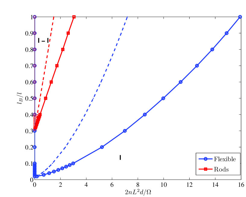
Figure 5: Comparison of the envelopes for isotropic-isotropic phase separation in symmetric mixtures of the oppositely charged flexible and rodlike polyelectrolytes. Dashed curves correspond to the spinodals and solid curves represent the binodals. The curves correspond to $N=1000,\;\tilde{d}=1/50,\;\sigma=0.1$. “I” and “I-I” denote one-phase isotropic and two-phase isotropic-isotropic coexistence regimes, respectively.

In Fig. 5, we have compared the spinodal phase boundaries for flexible and rodlike symmetric polyelectrolyte mixtures in a salt-free, counterion-free situation. It is clear that for these weakly charged polyelectrolyte systems (characterized by $4\pi l_{B}\sigma^{2}\rho<1$) the isotropic-isotropic coexistence regime is broader in the case of flexible symmetric mixtures in comparison with rodlike mixtures. As all the other contributions to the free energies of the two systems are the same except the electrostatic contributions, it is clear that the electrostatic driving force is stronger in the case of flexible polyelectrolytes than rodlike polyelectrolytes. We note that these numerical results are consistent with the simple scaling arguments presented in the introduction.

III.2 Full Phase Diagram

From the results presented and discussions so far, it is clear that electrostatics drives macrophase separation in the isotropic phase and also stabilizes the nematic phase. So, in principle, isotropic-isotropic, isotropic-nematic and/or nematic-nematic phase transitions can take place in symmetric mixtures of rodlike polyelectrolytes. Similar to the isotropic-isotropic phase calculations considered above, we consider the extra possibilities of nematic-isotropic and nematic-nematic coexistence, where the orientational order parameter in each phase is determined during the minimization of the total free energy density of the phase separated system.

For the quasi-one component system without counterions (cf. Eq. 53), we minimize the total free energy density written as

$$f_{total} = \frac{c_{p}^{\text{II}}-c_{p}}{c_{p}^{\text{II}}-c_{p}^{\text{I}}}f\left\{c_{p}^{\text{I}},\alpha^{\text{I}}\right\}+\frac{c_{p}-c_{p}^{\text{I}}}{c_{p}^{\text{II}}-c_{p}^{\text{I}}}f\left\{c_{p}^{\text{II}},\alpha^{\text{II}}\right\},$$ (60)

where the variational parameters $\alpha^{\text{I}}$ and $\alpha^{\text{II}}$ for the phases I and II, respectively, are obtained by numerically minimizing (using Brent’s methodnumerical_recipe ) the free energy density of the phase ($f\left\{c_{p}^{\text{I}}\right\}$ and $f\left\{c_{p}^{\text{II}}\right\}$ for the phases I and II, respectively, given by Eqs. 44 - 46) at the given monomer densities ($c_{p}^{\text{I}}$ and $c_{p}^{\text{II}}$ for the phases I and II, respectively). A similar approach can be taken in quasi two-dimensional systems that include counterions. The motivation behind carrying out such calculations is the fact that all the phase transitions that we have considered thus far (i.e., isotropic-isotropic and isotropic-nematic) are subsets of these more “general” calculations. Unfortunately, such high dimensional optimizations are computationally demanding, so we have looked for opportunities to accelerate the construction of full phase diagrams.

In a complementary set of calculations, we have considered isotropic-nematic and isotropic-isotropic phase transitions separately. It was found that the results of the “general” calculations described above exactly match the results of our isotropic-nematic and the isotropic-isotropic calculations (data not presented here). Through such calculations, we have also established that there are no regions of nematic-nematic coexistence, so the various phase diagrams can be mapped out by tracking individual I-I and I-N boundaries.

The phase diagrams presented in the remaining sections were obtained by the above technique and are presented in Figs. 6 and 7, respectively in the absence and presence of counterions. Overall, the results of these calculations are in qualitative agreement with the picture presented in Fig. 1. Some important features of the full phase diagram are discussed below.

III.2.1 Phase diagram without counterions

In Fig. 6, we have plotted the phase diagram for symmetric mixtures of oppositely charged rodlike polyelectrolytes in the absence of counterions. In the figure, the linear charge density is varied to explore the effect of electrostatics on the phase boundaries. From Fig. 6a, it is clear that the coexisting densities in the two phases decrease from the uncharged case with an increase in the charge densities (compare the results for $\sigma=0,0.02$ and $0.04$). However, a further increase in the charge density leads to three distinct regimes corresponding to the low, intermediate and high values of $l_{B}$. For very low values of the Bjerrum length ($l_{B}/l\rightarrow 0$), the coexisting phases are isotropic and nematic phases. Note that in this regime the coexisting densities for the isotropic and nematic phases for the polyelectrolyte systems are close to that for the neutral system.

For high values of the Bjerrum length (close to unity) and high charge densities such as $\sigma=0.08,0.1$ in Fig. 6a, completely ordered nematic phase becomes one of the coexisting phases. However, we haven’t been able to compute the densities of the coexisting phases in this regime due to the numerical issues discussed in subsection F above.

For intermediate values of $l_{B}$, there are regimes (e.g., $l_{B}/l\in 0.1-0.6$ for $\sigma=0.1$ in Fig. 6a), where isotropic-isotropic coexistence and isotropic-nematic phase separation can be separately realized by varying the concentration of the rodlike polyelectrolytes in solution. With an increase in $l_{B}$ in this regime, three phase coexistence (isotropic-isotropic-completely ordered nematic) can be realized in these systems. Moreover, the value of $l_{B}$ at which the three phase coexistence takes place is dependent on the linear charge density of the polyelectrolytes. In fact, the Bjerrum length at which the three phase coexistence takes place decreases with an increase in the linear charge density of the rods (compare the results for $\sigma=0.08$ and $\sigma=0.1$ in Fig. 6a). Note that in this intermediate regime, the entropic effects driving the isotropic-nematic transition are comparable in strength with the energetic effects (coming from electrostatics), but the system quickly evolves into a broad isotropic-nematic phase envelope upon increasing $l_{B}$. This leads to a sharp increase in the density of the coexisting nematic phase (see the plots for $\sigma=0.08$ and $\sigma=0.1$ in Fig. 6a). A further increase in $l_{B}$ leads to the completely ordered nematic phase as a coexisting phase. In order to keep track of the degree of alignment of the rods in the nematic phase in Fig. 6a, we have plotted the order parameter in Fig. 6b.

From Fig. 6b, it is clear that the order parameter increases with an increase in $l_{B}/l$, which is in agreement with the stability analysis carried out in this paper. Hence, the numerical results support the prediction that electrostatics favor orientational ordering.

III.2.2 Effect of counterions

In contrast to the phase diagram obtained in the absence of the counterions, the phase diagram in the presence of counterions depends on the total number density of the rodlike polyelectrolytes and correspondingly on the number of counterions in the system. In order to conduct a systematic study, we have carried out two sets of calculations. In the first set, we vary the linear charge density of the polyelectrolytes while keeping the total number density of the rodlike polyelectrolytes fixed at a particular value. In the second set, the total number density of the rods is varied keeping the linear charge density fixed at a particular value. So, in both the sets, the total number density of counterions is varied.

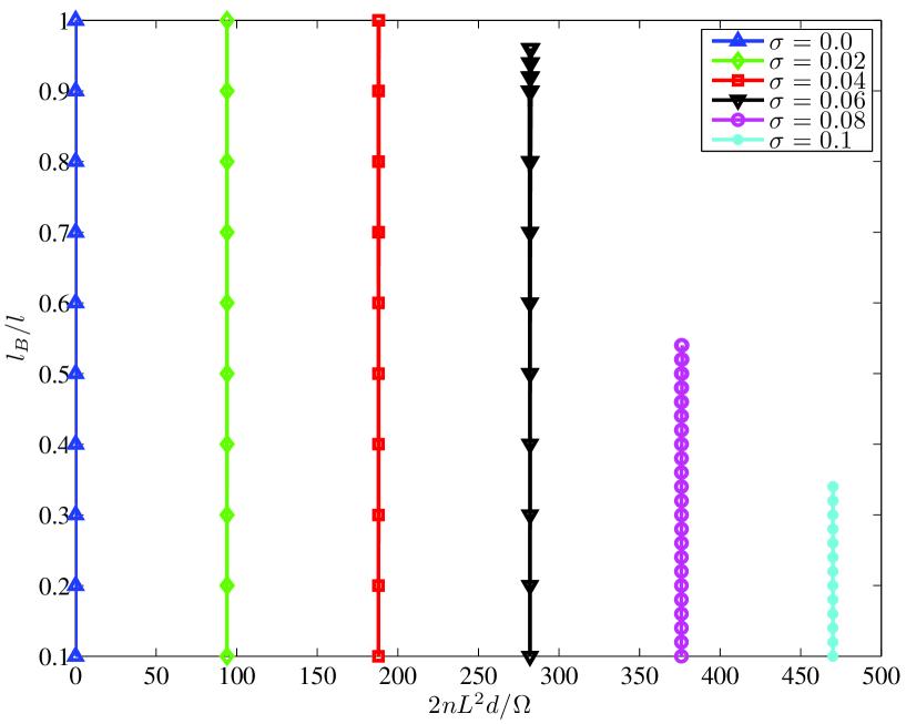
Figure 8: Counterion densities in the two coexisting phases shown in Fig. 7. The counterions are uniformly distributed between the two phases for these set of parameters.

Fig. 7 presents the results of the first set of calculations. Comparing Fig. 7 with Fig. 6, we observe that the qualitative features of the phase diagram in the presence of counterions remain the same as in the absence of counterions. Furthermore, Fig. 8 presents the number densities of the counterions in the coexisting phases. It is found that counterions are uniformly distributed between the two phases for these values of linear charge densities and the Bjerrum’s length.

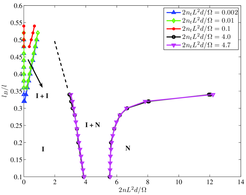
Figure 9: Effect of the total number density of rodlike polyelectrolytes on the phase diagram in symmetric mixtures in the presence of counterions and at fixed linear charge density. These plots correspond to $N=1000,\;d/l=1/50$ and $\sigma=0.1$. Dashed lines in Fig. (a) correspond to the boundary beyond which the isotropic phase becomes unstable and the completely ordered nematic phase becomes one of the coexisting phases.

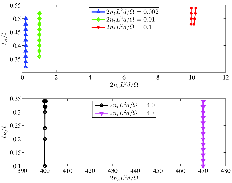
Figure 10: Counterion densities in the coexisting phases corresponding to I-I and I-N phase transitions as shown in Fig. 9. In these figures, the right branch of each coexisting curve corresponds to the counterion density in the phase dense in rodlike polyelectrolytes (coacervate). It is shown that for strong enough electrostatics, the counterions also phase segregate and the counterion density is higher in the dense phase (see the results for $2n_{t}L^{2}d/\Omega=0.1$). These plots correspond to $N=1000,\;d/l=1/50$ and $\sigma=0.1$.

The results for the second set of calculations are shown in Figs. 9 and 10, where the total number density of polyelectrolytes is changed for a particular value of the linear charge density. These results show the isotropic-isotropic and isotropic-nematic coexistence regimes just like the ones seen in the absence of counterions in Fig. 6. In these calculations, the change in the total number densities of the polyelectrolytes leads to a change in the total number density of the counterions. The effect of varying the total number density of the polyelectrolytes and counterions on the phase boundaries can be explained as follows. As already discussed, the origin of the isotropic-nematic transition for neutral rods near the overlap concentration or for very low values of $l_{B}$ ($l_{B}/l\rightarrow 0$) is entropic and is nearly independent of electrostatics. Hence, the presence of counterions does not affect these boundaries (compare the phase boundaries for $2n_{t}L^{2}d/\Omega=4$ and $4.7$). However, the origin of the isotropic-isotropic transition at low number density of polyelectrolytes is electrostatically driven and is strongly dependent on the presence of the counterions. The width of this particular coexistence regime can be tuned by changing the number of counterions. In particular, the coexistence regimes shrink with an increase in the number of counterions due to the screening of electrostatic interactions(compare $2n_{t}L^{2}d/\Omega=0.002,0.01$ and $0.1$ in Fig. 9). Note that the results for the isotropic-isotropic phase transition in Fig. 9 are the same as in Fig. 4.

Figure 10 shows the counterion distribution in the coexisting phases. Consistent with our prior results, it is evident that the counterions also phase segregate at high Bjerrum length with a higher density in the concentrated (coacervate) phase.

IV Conclusions

We have studied the phase behavior of salt-free symmetric mixtures of oppositely charged rodlike polyelectrolytes using the random phase approximation. In this work, we have focused on weak polyelectrolytes in the regime $l_{B}/l<1$ to avoid complications arising from possible counterion condensation. For a variety of symmetric mixtures, we have computed the phase boundaries for regions of isotropic-isotropic and isotropic-nematic coexistence. We were not able to identify any regions of nematic-nematic coexistence in these symmetric systems.

Our stability analysis and numerical results for coexistence curves reveal that electrostatic interactions favor nematic ordering of the rodlike components in solution. Nonetheless, the screening of these electrostatic interactions by higher concentrations of counterions weakens or destroys this ordering. It is shown that the phase boundaries for symmetric mixtures containing oppositely charged rodlike polyelectrolytes are dependent on the electrostatic interaction strengths characterized by the linear charge density, $\sigma$, and the Bjerrum length, $l_{B}$. In particular, it is demonstrated that at low electrostatic interaction strengths (i.e., $l_{B}/l\rightarrow 0,\>\sigma\rightarrow 0$), the densities in the coexisting isotropic and nematic phases decrease with an increase in the linear charge density of the polyelectrolytes in the absence of counterions. However, an increase in the electrostatic interaction strength by increasing $\sigma$ leads to three distinct regimes characterized by $l_{B}/l$. At low $l_{B}/l$ (close to zero), a narrow region of isotropic-nematic coexistence prevails, whose origin lies in the entropy of the system. On the other hand, at relatively high $l_{B}/l$ (close to unity), the completely ordered nematic phase becomes one of the coexisting phases. However, its origin lies in the electrostatic attraction between oppositely charged polyelectrolytes. At intermediate values of $l_{B}$, isotropic-isotropic or isotropic-nematic coexistence can prevail depending on the concentration of the polyelectrolytes. Also, in this regime, at a particular value of $l_{B}$, three phases (low density isotropic, moderate density isotropic, and high density nematic) coexist with each other. The value of $l_{B}$ at which the three phase coexistence takes place depends sensitively on the linear charge density of the polyelectrolytes.

We have also investigated the effect of counterions on the phase coexistence boundaries (isotropic-isotropic and isotropic-nematic). Comparison of the results for the systems with and without counterions reveals that sufficiently high concentrations of counterions suppress both isotropic-isotropic and isotropic-nematic coexistence. A key prediction of theory is the result that the concentration of counterions in the dense (or coacervate) phase is slightly higher than in the dilute (or supernatant) phase. Also, comparison of the phase separation boundaries between comparable rodlike and flexible polyelectrolyte mixtures reveals that the isotropic-isotropic macrophase separation regime is broader in the case of weakly charged flexible polyelectrolytes.

Furthermore, in this work, we have limited ourselves to the phase separation regime in the mixtures containing weakly charged polyelectrolytes close to the critical point. We have found that the critical points for the isotropic-isotropic and isotropic-nematic phase transitions exist at very low number density of rods ($n/\Omega\sim 1/L^{2}d$) and weak electrostatic interaction strengths (i.e., $l_{B}/l\ll 1$). At this point, we remark on the range of validity of the theory to describe the phase boundaries and some of the future directions. There are three key issues, which limits the validity of the theory. In future, we’ll extend the theory to higher electrostatic interaction strengths by addressing the issues mentioned below.

First issue is the use of the random phase approximation (RPA) to compute the contribution to the free energy coming from the electrostatic correlations. A typical way to judge the validity of the RPA is to compare the mean field contribution with the correlation term in the free energy. Due to the fact that the mean field contribution to the free energy coming from the electrostatics is zero and correlation terms beyond the RPA are not available, the range of validity of RPA can’t be inferred directly. However, general consensusborue_complexation ; muthu_double ; joanny_leibler ; kaji_kanaya is that the RPA for flexible polymers is valid for concentrations above the overlap concentration. In this work, the coacervate phase has concentration above the overlap concentration and the supernatant phase is very dilute. Indeed, the supernatant phase is not well described by the RPA. On the other hand, the RPA is suitable for a very good quantitative description of the phase boundary describing the coacervate phase. Remarkably, the RPA predicts a supernatant phase with almost zero density in qualitative agreement with the experimentsdubin_review ; pe_complex_reviews ; voorn_review ; veis_complexation ; kabanov_work1 ; kabanov_work2 ; dautzenberg_work1 ; pogodina_work ; dautzenberg_work2 . Furthermore, the RPA describing the coacervate phase boundary in the case of flexible polyelectrolyte mixtures has been compared extensively with the experimentsleibler_borukhov and simulationsjay_yuri_2 . Indeed, agreement between the theory, simulations and experiments is remarkable. In order to go beyond the RPA, Hartree approximationglenn_book can be used, which can provide a more quantiative description for the supernatant phase also. However, we leave it for future work.

Second issue arises due to the use of the Onsager second virial approach to describe the steric effects in the case of long rods. It is well-knownedwardsbook ; straley_review that the approach only works in the limit of very long aspect ratio of the rods. In fact, the limit of validity of the Onsager corresponds to $L/d\gg 10$. Furthermore, the second virial approach is strictly valid for low number density of the rods. For dense systems, higher order terms needs to be considered. For very long rods, the isotropic-nematic and isotropic-isotropic phase transitions occur at low enough number densities of the rods (which is of the order of overlap concentration). This is the reason the second virial approach is able to correctly predict these phase transitions at low electrostatic interaction strengths. However, an increase in the electrostatic interaction strength causes the density of the coacervate phase to increase and the virial approach breaks down. This deficiency of the theory can be removed by considering the effect of higher order termsparsons_paper ; lee_higher , which we’ll consider in future.

Third issue is the ignorance of charge renormalization while describing phase separation. In this work, the phase separation regime corresponding to very low electrostatic interaction strengths is described assuming that there is no counterion adsorption on the polyelectrolytes. In this regime, the issue of charge renormalization during phase separation can be safely ignored. However, with the increase in the electrostatic interaction strength, counterions can adsorb on the polyelectrolytes and modulate their charge. For this part of the phase diagram, the degree of ionization for each polyelectrolyte in each phase needs to be computed, while equating the chemical potential and pressure of each component in the two phaseslevin_charge_regularization ; muthu_charge_regularization . In other words, the possibility of different degree of ionizations in daughter phases needs to be explored. In this work, we have limited the theoretical study to $l_{B}/l<1$, where issue of counterion adsorption can be safely ignored.

A related issue is the consideration of ionic clusters (such as dipoles, quadrapoles etc.) formed as a result of strong electrostatic attraction between different oppositely charged components. It has been shownfisher_levin ; fisher in the literature that the issue of ion-pairing has to be taken into account in the case of hard sphere model for simple electrolytes (also known as restricted primitive model (RPM)) to correctly match the simulation results in the critical regime. This is a manifestation of the fact that the critical point for the RPM, as predicted by the Debye-Hückel theory, correspondsfisher_levin to $q^{2}l_{B}^{\star}/a=16$, where $q$ is the charge per sphere, $l_{B}^{\star}$ is the Bjerrum length at the critical point and $a$ is the diameter of the hard spheres. For symmetrical electrolytes, $a$ is the same for both kinds of charged spheres. Also, for monovalent electrolytes, $q=1$ and the critical point exists at very low temperature such that $l_{B}^{\star}/a=16$. At such low temperatures, indeed one has to extend the Debye-Hückel theory (which is a RPA like) by including atleast dipolar interactions in the regime near the critical point. However, in contrast to the symmetric electrolytic mixtures, the phase separation regime close to the critical point in the case of mixtures containing long flexible or rodlike polyelectrolytes can be well described within RPA without any consideration of ion-ion, ion-polyelectrolyte (which is the same as the counterion adsorption) or polyelectrolyte-polyelectrolyte pairs. This is an outcome of the fact that now the phase separation takes place at relatively higher temperatures and low densities. In this regime, the mixtures of oppositely charged polyelectrolytes behave as weakly correlated liquidsrubinstein_pairing . However, if we increase the electrostatic interaction strength and go far from the critical regime, there is a competition for pairing between different oppositely charged species. A rough estimate for the minimum driving force for pairing between the ions is given by Bjerrum’s theoryebeling_work ; levin_review of ion-pairs. According to the theory, life time of the paired state in the case of two oppositely charged ions (while undergoing thermal motion) significantly increases when $q^{2}l_{B}/r>2$, $r$ being the distance between the ions. In this regime, the electrostatic attraction takes over the thermal energy of ions and ion-ion pair (or dipole) needs to be considered as a new species. This relation can be cast in terms of number density of ions ($=n_{c}/\Omega$) by using $r\sim(n_{c}/\Omega)^{-1/3}$ so that $q^{2}l_{B}/l>1/(n_{c}/\Omega)^{1/3}$. Issue of ion pairs/clusters formed as a result of binding, which involves charged monomers is more suble compared to the issue of pairing in small ions.

However, we can estimate the regime, where one has to explicitly consider the binding between the polyelectrolytes and oppositely charged counterions or polyelectrolytes. Carrying out a single chain analysis, it has been shown that the binding of counterions on flexible and rodlike polyelectrolytes becomes importantmanning ; counterion_adsorption_muthu roughly around $l_{B}/l>1$. Similarly, an analysis of the system containing two oppositely charged flexible polyelectrolyteszhaoyang_complex reveals that the complexation takes place only for strong electrostatic interaction strengths (i.e., $\sigma^{2}l_{B}>1$). For rodlike polyelectrolytes, the electrostatic interaction strength required for complexation needs to be stronger compared to the flexible polyelectrolytes due to weaker (logarithmic) electrostatic potential for rodlike polymers. These single chain analyses provide a clear picture about the dilute solution regime. In the regime above the overlap concentration for polymers, situation is more complicated and one has to consider the multi-chain effects. However, one can carry out a mean-field analysismonica_complexation_2 ; semenov_rubinstein to estimate the fraction of charged monomers involved in binding (say, $\Gamma$). It can be readily shownmonica_complexation_2 that the fraction is given by the relation $\Gamma/(1-\Gamma)^{2}=(\sigma/l)\left[c_{p}/(2Ld)\right]\exp(|E/k_{B}T|)$, $E/k_{B}T\sim l_{B}$ being the energy gain per pair. In this work, we have considered weakly charged polyelectrolyte solutions at very low electrostatic interaction strengths so that the fraction of charged monomers involved in pairing is close to zero.

At present we are not aware of experimental data sets sufficient for a comprehensive test of the theoretical predictions made here. With this aim, we welcome interactions with experimental groups to define appropriate systems and experimental protocols.

APPENDIX A : Partition function for mixtures of rodlike polyelectrolytes

Here, we present the details of our derivation of the free energy for the mixtures of rodlike polyelectrolytes in the presence of counterions as described in Section II. Different parameters representing the number of rods and counterions, length and diameter of the rods, and charge along the rods have already been described in Section II. In terms of these parameters, the partition function can be written as

$$Z = \frac{\prod_{k=+,-}\prod_{j=1}^{n_{k}}\left[\int_{p_{k}(\mathbf{u}_{j},\hat{\mathbf{n}})}d\mathbf{r}_{j}d\mathbf{u}_{j}\right]}{\prod_{k=+,-}n_{k}!\prod_{j^{\prime}=c+,c-}n_{j^{\prime}}!}\prod_{j^{\prime}=c+,c-}\prod_{j^{\prime\prime}=1}^{n_{j^{\prime}}}\int d\mathbf{r}_{j^{\prime\prime}}\exp\left[-\frac{H_{int}}{k_{B}T}\right]$$ (A-1)

where

$$\frac{H_{int}}{k_{B}T} = \frac{H_{w}}{k_{B}T}+\frac{H_{e}}{k_{B}T},$$ (A-2)

$$\frac{H_{w}}{k_{B}T} = \frac{1}{2}\sum_{j=1}^{n_{+}+n_{-}}\sum_{k=1}^{n_{+}+n_{-}}W(\mathbf{r}_{j},\mathbf{u}_{j},\mathbf{r}_{k},\mathbf{u}_{k}),$$ (A-3)

$$\frac{H_{e}}{k_{B}T} = \frac{l_{B}}{2}\int d\mathbf{r}\int d\mathbf{r}^{\prime}\frac{\hat{\rho}_{e}(\mathbf{r})\hat{\rho}_{e}(\mathbf{r}^{\prime})}{|\mathbf{r}-\mathbf{r}^{\prime}|}.$$ (A-4)

Here, $p_{k}(\mathbf{u}_{j},\hat{\mathbf{n}})$ for $k=+,-$ is the probability of finding a rod of type $k$ oriented along unit vector $\mathbf{u}_{j}$ when the director is taken to be along the unit vector $\hat{\mathbf{n}}$. Subscript $p_{k}(\mathbf{u},\hat{\mathbf{n}})$ under the integral symbol means that the integration need to be carried out under the constraint that the orientational distribution function for the positive and negative rods are $p_{+}(\mathbf{u},\hat{\mathbf{n}})$ and $p_{-}(\mathbf{u},\hat{\mathbf{n}})$, respectively. Also, hamiltonian $H_{int}$ is divided into contributions coming from the short range excluded volume interactions ($H_{w}$) and the long range electrostatic interactions ($H_{e}$). Furthermore, in the expression for $H_{w},W(\mathbf{r}_{j},\mathbf{u}_{j},\mathbf{r}_{k},\mathbf{u}_{k})$ characterizes the excluded volume interactions between two rods whose centers are located at $\mathbf{r}_{j}$ and $\mathbf{r}_{k}$ with their axes oriented along $\mathbf{u}_{j}$ and $\mathbf{u}_{k}$, respectively. Also, $l_{B}$ is Bjerrum length and $\hat{\rho}_{e}$ in the expression for $H_{e}$ is the local charge density defined as

$$\hat{\rho}_{e}(\mathbf{r}) = Z_{+}\sigma_{+}\hat{\rho}_{+}(\mathbf{r})+Z_{-}\sigma_{-}\hat{\rho}_{-}(\mathbf{r})+\sum_{j^{\prime}=c+,c-}Z_{j^{\prime}}\hat{\rho}_{j^{\prime}}(\mathbf{r})$$ (A-5)

$$\hat{\rho}_{k}(\mathbf{r}) = N_{k}\sum_{j=1}^{n_{k}}\frac{1}{L_{k}}\int_{-L_{k}/2}^{L_{k}/2}ds_{j}\,\delta(\mathbf{r}_{j}+s_{j}\mathbf{u}_{j}-\mathbf{r}),\quad\mbox{for}\quad k=+,-,$$ (A-6)

$$\hat{\rho}_{j^{\prime}}(\mathbf{r}) = \sum_{j^{\prime\prime}=1}^{n_{j^{\prime}}}\delta(\mathbf{r}-\mathbf{r}_{j^{\prime\prime}}),\quad\mbox{for}\quad j^{\prime}=c+,c-,$$ (A-7)

where $Z_{\gamma}$ is the valency (with sign) of the charged species of type $\gamma$ and $N_{k}$ is the number of monomers for the rod of type $k$ so that $L_{k}=N_{k}l_{k}$, $l_{k}$ being the monomer length. Also, $s_{j}$ in the expression for $\hat{\rho}_{k}(\mathbf{r})$ is the contour variable used to locate any monomer along the $j^{th}$ rod of type $k$. In order to proceed further, we rewrite $Z$ as

$$Z = Z_{o}\left<\exp\left[-\frac{H_{int}}{k_{B}T}\right]\right>_{p_{+},p_{-}}$$ (A-8)

where $Z_{o}$ is the partition function for a non-interacting system with the same orientational distributions (i.e., $p_{+},p_{-}$) and also the normalization factor in the expression for $Z$, given by

$$Z_{o} = \exp\left[-\frac{F_{o}}{k_{B}T}\right]=\frac{\prod_{k=+,-}\prod_{j=1}^{n_{k}}\left[\int_{p_{k}(\mathbf{u},\hat{\mathbf{n}})}d\mathbf{r}_{j}d\mathbf{u}_{j}\right]}{\prod_{k=+,-}n_{k}!\prod_{j^{\prime}=c+,c-}n_{j^{\prime}}!}\int\prod_{j^{\prime}=c+,c-}\prod_{j^{\prime\prime}=1}^{n_{j^{\prime}}}d\mathbf{r}_{j^{\prime\prime}}$$ (A-9)

$$= \prod_{\gamma=+,-,c+,c-}\left[\frac{\Omega^{n_{\gamma}}}{n_{\gamma}!}\right]\prod_{k=+,-}\prod_{j=1}^{n_{k}}\int_{p_{k}(\mathbf{u},\hat{\mathbf{n}})}d\mathbf{u}_{j}.$$

Using Stirling’s approximation for factorials $n!\simeq n(\ln n-1)$ and considering different ways of distributing $n_{k}$ rods for a given orientational probability distribution function $p_{k}(\mathbf{u}_{j},\hat{\mathbf{n}})$ along the surface of a unit sphereedwardsbook

$$\frac{F_{o}}{k_{B}T} = \sum_{j=+,-}n_{j}\int d\mathbf{u}_{j}p_{j}(\mathbf{u}_{j},\hat{\mathbf{n}})\ln\left[4\pi p_{j}(\mathbf{u}_{j},\hat{\mathbf{n}})\right]+\sum_{\gamma=+,-,c+,c-}n_{\gamma}\left[\ln\frac{n_{\gamma}}{\Omega}-1\right].$$ (A-10)

Also,

$$\left<\exp\left[-\frac{H_{int}}{k_{B}T}\right]\right>_{p_{+},p_{-}} = \frac{\prod_{k=+,-}\prod_{j=1}^{n_{k}}\left[\int_{p_{k}(\mathbf{u}_{j},\hat{\mathbf{n}})}d\mathbf{r}_{j}d\mathbf{u}_{j}\right]\prod_{j^{\prime}=c+,c-}\prod_{j^{\prime\prime}=1}^{n_{j^{\prime}}}\int d\mathbf{r}_{j^{\prime\prime}}\exp\left[-\frac{H_{int}}{k_{B}T}\right]}{\prod_{k=+,-}\prod_{j=1}^{n_{k}}\left[\int_{p_{k}(\mathbf{u}_{j},\hat{\mathbf{n}})}d\mathbf{r}_{j}d\mathbf{u}_{j}\right]\prod_{j^{\prime}=c+,c-}\prod_{j^{\prime\prime}=1}^{n_{j^{\prime}}}\int d\mathbf{r}_{j^{\prime\prime}}}.$$

Using the Hubbard-Stratonovich transformationglenn_book for the electrostatic part i.e., $H_{e}$ and using Fourier transform defined for any arbitrary function $f(\mathbf{r})$ by

$$f(\mathbf{r}) = \int\frac{d^{3}\mathbf{q}}{(2\pi)^{3}}f_{q}e^{i\mathbf{q}\cdot\mathbf{r}},$$ (A-12)

the partition function can be written as

$$\frac{Z}{Z_{o}} = \frac{\int\prod_{q}D[\psi_{q}]\exp\left[-\frac{1}{2}\int\frac{d^{3}\mathbf{q}}{(2\pi)^{3}}\psi_{q}\frac{q^{2}}{4\pi l_{B}}\psi_{-q}+\sum_{j^{\prime}=c+,c-}n_{j^{\prime}}\ln Q_{j^{\prime}}\left\{\psi_{q}\right\}\right]}{\int\prod_{q}D[\psi_{q}]\exp\left[-\frac{1}{2}\int\frac{d^{3}\mathbf{q}}{(2\pi)^{3}}\psi_{q}\frac{q^{2}}{4\pi l_{B}}\psi_{-q}\right]}$$

$$\frac{\prod_{k=+,-}\prod_{j=1}^{n_{k}}\left[\int_{p_{k}(\mathbf{u}_{j},\hat{\mathbf{n}})}d\mathbf{r}_{j}d\mathbf{u}_{j}\right]\exp\left[-\frac{H_{w}}{k_{B}T}+i\sum_{k=+,-}\int\frac{d^{3}\mathbf{q}}{(2\pi)^{3}}\psi_{q}Z_{k}\sigma_{k}\rho_{k,-q}\right]}{\prod_{k=+,-}\prod_{j=1}^{n_{k}}\left[\int_{p_{k}(\mathbf{u}_{j},\hat{\mathbf{n}})}d\mathbf{r}_{j}d\mathbf{u}_{j}\right]}$$

where

$$\rho_{k,q} = \int\,d\mathbf{r}\hat{\rho}_{k}(\mathbf{r})e^{i\mathbf{q}\cdot\mathbf{r}}=\sum_{i=1}^{n_{k}}N_{k}e^{i\mathbf{q}.\mathbf{r}_{i}}\frac{\sin\left[\left(\mathbf{q}\cdot\mathbf{u}_{i}\right)L_{k}/2\right]}{\left[\left(\mathbf{q}\cdot\mathbf{u}_{i}\right)L_{k}/2\right]},\quad\mbox{for}\quad k=+,-$$ (A-14)

and

$$Q_{j^{\prime}}\left\{\psi_{q}\right\} = \frac{1}{\Omega}\int d\mathbf{r}\exp\left[i\int\frac{d^{3}q}{(2\pi)^{3}}\psi_{q}Z_{j^{\prime}}e^{i\mathbf{q}\cdot\mathbf{r}}\right]$$ (A-15)

So far the partition function is exact. However, evaluation of the exact partition function is a tedious task. Useful insights can be obtained by invoking the following approximations.

From Eq.  A-15

$$\sum_{j^{\prime}=c+,c-}\ln Q_{j^{\prime}}^{n_{j^{\prime}}}\left\{\psi_{q}\right\} \simeq \sum_{j^{\prime}=c+,c-}\ln\left[1-\frac{Z_{j^{\prime}}^{2}n_{j^{\prime}}}{2\Omega}\int\frac{d^{3}q}{(2\pi)^{3}}\psi_{q}\psi_{-q}\right]$$ (A-16)

$$\simeq -\sum_{j^{\prime}=c+,c-}\frac{Z_{j^{\prime}}^{2}n_{j^{\prime}}}{2\Omega}\int\frac{d^{3}q}{(2\pi)^{3}}\psi_{q}\psi_{-q}.$$

Note here that the linear terms arising from the expansion of the exponential in $Q_{j^{\prime}}$ vanish in the sum due to the presence of oppositely charged counterions, i.e. $Z_{c+}=-Z_{c-}$. Furthermore, approximating the logarithm by the first term in the expansion in Eq.  A-16 is strictly valid for dilute concentrations of the counterions so that $n_{j^{\prime}}/\Omega$ is small. Using this approximation, Eq.  LABEL:eq:parti_all becomes

$$\frac{Z}{Z_{o}} = \frac{\int\prod_{q}D[\psi_{q}]\exp\left[-\frac{1}{8\pi l_{B}}\int\frac{d^{3}\mathbf{q}}{(2\pi)^{3}}\psi_{q}\left(q^{2}+\kappa^{2}\right)\psi_{-q}\right]}{\int\prod_{q}D[\psi_{q}]\exp\left[-\frac{1}{8\pi l_{B}}\int\frac{d^{3}\mathbf{q}}{(2\pi)^{3}}\psi_{q}q^{2}\psi_{-q}\right]}$$

$$\frac{\prod_{k=+,-}\prod_{j=1}^{n_{k}}\left[\int_{p_{k}(\mathbf{u}_{j},\hat{\mathbf{n}})}d\mathbf{r}_{j}d\mathbf{u}_{j}\right]\exp\left[-\frac{H_{w}}{k_{B}T}+i\sum_{k=+,-}\int\frac{d^{3}\mathbf{q}}{(2\pi)^{3}}\psi_{q}Z_{k}\sigma_{k}\rho_{k,-q}\right]}{\prod_{k=+,-}\prod_{j=1}^{n_{k}}\left[\int_{p_{k}(\mathbf{u}_{j},\hat{\mathbf{n}})}d\mathbf{r}_{j}d\mathbf{u}_{j}\right]}$$

where we have defined $\kappa^{2}=4\pi l_{B}\sum_{j^{\prime}}Z_{j^{\prime}}^{2}n_{j^{\prime}}/\Omega$ so that $\kappa^{-1}$ is the Debye length. Now the integrals over the spatial and orientational degrees of freedom under the constraint of the given distribution functions can be carried out using the approximation described in Ref. edwardsbook . To be explicit,

$$I_{p}\left\{\psi_{q}\right\} = \frac{\prod_{k=+,-}\prod_{j=1}^{n_{k}}\left[\int_{p_{k}(\mathbf{u}_{j},\hat{\mathbf{n}})}d\mathbf{r}_{j}d\mathbf{u}_{j}\right]\exp\left[-\frac{H_{w}}{k_{B}T}+i\sum_{k=+,-}\int\frac{d^{3}\mathbf{q}}{(2\pi)^{3}}\psi_{q}Z_{k}\sigma_{k}\rho_{k,-q}\right]}{\prod_{k=+,-}\prod_{j=1}^{n_{k}}\left[\int_{p_{k}(\mathbf{u}_{j},\hat{\mathbf{n}})}d\mathbf{r}_{j}d\mathbf{u}_{j}\right]}$$ (A-18)

$$= \frac{\prod_{k=+,-}\prod_{j=1}^{n_{k}}\left[\int_{p_{k}(\mathbf{u}_{j},\hat{\mathbf{n}})}d\mathbf{r}_{j}d\mathbf{u}_{j}\right]\left[1-\left\{1-\exp\left(-\frac{H_{w}}{k_{B}T}\right)\right\}\right]\exp\left[i\sum_{k}\int\frac{d^{3}\mathbf{q}}{(2\pi)^{3}}\psi_{q}Z_{k}\sigma_{k}\rho_{k,-q}\right]}{\prod_{k=+,-}\prod_{j=1}^{n_{k}}\left[\int_{p_{k}(\mathbf{u}_{j},\hat{\mathbf{n}})}d\mathbf{r}_{j}d\mathbf{u}_{j}\right]}$$

$$= 1-\frac{\prod_{k=+,-}\prod_{j=1}^{n_{k}}\left[\int_{p_{k}(\mathbf{u}_{j},\hat{\mathbf{n}})}d\mathbf{r}_{j}d\mathbf{u}_{j}\right]\left\{1-\exp\left(-\frac{H_{w}}{k_{B}T}\right)\right\}}{\prod_{k=+,-}\prod_{j=1}^{n_{k}}\left[\int_{p_{k}(\mathbf{u}_{j},\hat{\mathbf{n}})}d\mathbf{r}_{j}d\mathbf{u}_{j}\right]}$$

$$-\frac{1}{2}\frac{\prod_{k=+,-}\prod_{j=1}^{n_{k}}\left[\int_{p_{k}(\mathbf{u}_{j},\hat{\mathbf{n}})}d\mathbf{r}_{j}d\mathbf{u}_{j}\right]\left[\int\frac{d^{3}\mathbf{q}}{(2\pi)^{3}}\psi_{q}\sum_{k}Z_{k}\sigma_{k}\rho_{k,-q}\right]^{2}}{\prod_{k=+,-}\prod_{j=1}^{n_{k}}\left[\int_{p_{k}(\mathbf{u}_{j},\hat{\mathbf{n}})}d\mathbf{r}_{j}d\mathbf{u}_{j}\right]}+\cdots$$

where we have ignored a cross-term between the excluded volume interactions and the electrostatics part to keep the calculations analytically tractable. Now, assuming that the excluded volume interactions between the rods occur independently of each other, second term in the series in Eq.  A-18 can be evaluated.edwardsbook Third term in the series is also straigthforward to evaluate after plugging the expression for $\rho_{k,q}$ given in Eq.  A-14. Now, exponentiating the series

$$\frac{Z}{Z_{o}} = \exp\left[-\frac{1}{2\Omega}\sum_{j,k=+,-}^{\prime}n_{j}n_{k}\int d\mathbf{u}\int d\mathbf{u}^{\prime}p_{j}(\mathbf{u},\hat{\mathbf{n}})\left[2L_{j}L_{k}d|\mathbf{u}\times\mathbf{u}^{\prime}|\right]p_{k}(\mathbf{u}^{\prime},\hat{\mathbf{n}})\right]$$

$$\frac{\int\prod_{q}D[\psi_{q}]\exp\left[-\frac{1}{8\pi l_{B}}\int\frac{d^{3}\mathbf{q}}{(2\pi)^{3}}\psi_{q}\left\{q^{2}+\kappa^{2}+\sum_{k=+,-}\kappa_{k}^{2}t_{k}(qL_{k})\right\}\psi_{-q}\right]}{\int\prod_{q}D[\psi_{q}]\exp\left[-\frac{1}{8\pi l_{B}}\int\frac{d^{3}\mathbf{q}}{(2\pi)^{3}}\psi_{q}q^{2}\psi_{-q}\right]}$$

where we have defined $\kappa_{k}^{2}=4\pi l_{B}Z_{k}^{2}\sigma_{k}^{2}L_{k}^{2}n_{k}/\Omega$ and

$$t_{k}(qL_{k}) = \int d\mathbf{u}p_{k}(\mathbf{u},\hat{\mathbf{n}})\left[\frac{\sin\left[\left(\mathbf{q}.\mathbf{u}\right)L_{k}/2\right]}{\left[\left(\mathbf{q}.\mathbf{u}\right)L_{k}/2\right]}\right]^{2},\quad\mbox{for}\quad k=+,-.$$ (A-20)

Also, the primed superscript means that the $j=k$ terms are omitted from the double sum. By carrying out the Gaussian functional integrals over $\psi_{q}$ and subtracting out the free energy in the low density limit, Eq. 11 is obtained.

APPENDIX B : Limiting cases for the electrostatic part of the free energy of the isotropic phase

Here, we provide a derivation of the approximate form of the electrostatic contribution to the free energy of the isotropic phase in the limiting cases of $L_{k}\rightarrow\infty$ (cf. Eqs. 22 and  23). In particular, we focus on the logarithmic corrections to the free energy of the mixture of charged rods as already described using scaling analysis in section  II.1. The electrostatic component of the free energy is given by

$$\frac{F_{e}\left\{L_{k}\rightarrow\infty\right\}}{k_{B}T} = \frac{\Omega}{2}\int\frac{d^{3}\mathbf{q}}{(2\pi)^{3}}\left\{\ln\left[1+\frac{\kappa^{2}}{q^{2}}+\frac{\pi\kappa_{p}^{2}}{q^{3}}\right]-\frac{\kappa^{2}}{q^{2}}-\frac{\pi\kappa_{p}^{2}}{q^{3}}\right\}$$ (B-1)

For weakly charged rods so that $\kappa_{p}^{2}\ll 1$,

$$\frac{F_{e}\left\{L_{k}\rightarrow\infty\right\}}{k_{B}T} = \frac{\Omega}{2}\int\frac{d^{3}\mathbf{q}}{(2\pi)^{3}}\left\{\ln\left[1+\frac{\kappa^{2}}{q^{2}}\right]-\frac{\kappa^{2}}{q^{2}}\right\}-\frac{\Omega}{2}\int\frac{d^{3}\mathbf{q}}{(2\pi)^{3}}\frac{\pi\kappa_{p}^{2}\kappa^{2}}{q^{3}\left(q^{2}+\kappa^{2}\right)}$$ (B-2)

$$-\frac{\Omega}{4}\int\frac{d^{3}\mathbf{q}}{(2\pi)^{3}}\frac{\pi^{2}\kappa_{p}^{4}}{q^{2}\left(q^{2}+\kappa^{2}\right)^{2}}+\cdots$$

$$\simeq -\frac{\Omega\kappa^{3}}{12\pi}-\frac{\Omega\kappa_{p}^{2}}{4\pi}\ln\left[\frac{\kappa}{q}\right]_{q\rightarrow 0}-\frac{\Omega\pi\kappa_{p}^{4}}{32\kappa^{3}}+\cdots,$$

which is Eq.  22. On the other hand, for strongly charged rods in weakly screened solutions $\kappa_{p}^{2}\gg 1$ and $\kappa\rightarrow 0$. In this limit,

$$\frac{F_{e}\left\{L_{k}\rightarrow\infty\right\}}{k_{B}T} \simeq \frac{\Omega}{2}\int\frac{d^{3}\mathbf{q}}{(2\pi)^{3}}\left\{\ln\left[1+\frac{\kappa^{2}}{q^{2}}\right]-\frac{\kappa^{2}}{q^{2}}\right\}$$

$$+\frac{\Omega}{2}\int\frac{d^{3}\mathbf{q}}{(2\pi)^{3}}\left\{\ln\left[1+\frac{\pi\kappa_{p}^{2}}{q^{3}}\left\{1-\frac{\kappa^{2}}{q^{2}}+\frac{\kappa^{4}}{q^{4}}\right\}\right]-\frac{\pi\kappa_{p}^{2}}{q^{3}}\right\}$$

$$= -\frac{\Omega\kappa^{3}}{12\pi}+\frac{\Omega}{2}\int\frac{d^{3}\mathbf{q}}{(2\pi)^{3}}\left\{\ln\left[1+\frac{\pi\kappa_{p}^{2}}{q^{3}}\right]-\frac{\pi\kappa_{p}^{2}}{q^{3}}\right\}+\frac{\Omega}{2}\int\frac{d^{3}\mathbf{q}}{(2\pi)^{3}}\ln\left[1-\frac{\frac{\kappa^{2}}{q^{2}}-\frac{\kappa^{4}}{q^{4}}}{1+\frac{\pi\kappa_{p}^{2}}{q^{3}}}\right]$$

$$= -\frac{\Omega\kappa^{3}}{12\pi}+\frac{\Omega}{2}\int\frac{d^{3}\mathbf{q}}{(2\pi)^{3}}\left\{\ln\left[1+\frac{\pi\kappa_{p}^{2}}{q^{3}}\right]-\frac{\pi\kappa_{p}^{2}}{q^{3}}\right\}-\frac{\Omega}{2}\int\frac{d^{3}\mathbf{q}}{(2\pi)^{3}}\frac{\frac{\kappa^{2}}{q^{2}}-\frac{\kappa^{4}}{q^{4}}}{1+\frac{\pi\kappa_{p}^{2}}{q^{3}}}+\cdots$$

$$= -\frac{\Omega\kappa^{3}}{12\pi}-\frac{\Omega\kappa_{p}^{2}}{6\pi}\ln\left[\frac{\sqrt{\pi}\kappa_{p}}{q}\right]_{q\rightarrow 0}+\frac{\Omega\kappa^{2}\kappa_{p}^{2/3}}{6\sqrt{3}\pi^{2/3}}-\frac{\Omega\kappa^{4}}{6\sqrt{3}\pi^{4/3}\kappa_{p}^{2/3}}-\frac{\Omega\kappa^{2}}{4\pi^{2}}\left[q\right]_{q\rightarrow\infty}+\cdots,$$

which is Eq.  23.

APPENDIX C : Partition function for mixtures of flexible polyelectrolytes

Here, we present the derivation of the free energy for mixtures of oppositely charged flexible polyelectrolytes in the presence of their counterions. The flexible polyelectrolytes are represented by continuous curves so that $\mathbf{R}_{jk}(s_{j})$ is the position vector of the $s^{th}$ monomer along the $j^{th}$ chain of type $k$. Furthermore, the contour lengths of chains of type $k$ is taken to be $L_{k}=N_{k}l_{k}$, $l_{k}$ being the Kuhn’s segment length. Accounting for the conformational degrees of freedom of the flexible chains by the path integral representation, the partition function for this system can be written as

$$Z = \frac{\prod_{k=+,-}\prod_{j=1}^{n_{k}}\int D\left[\mathbf{R}_{jk}\right]\exp\left[-\frac{H_{0}}{k_{B}T}\right]}{{\prod_{k=+,-}n_{k}!\prod_{j^{\prime}=c+,c-}n_{j^{\prime}}!}}\prod_{j^{\prime}=c+,c-}\prod_{j^{\prime\prime}=1}^{n_{j^{\prime}}}\int d\mathbf{r}_{j^{\prime\prime}}\exp\left[-\frac{H_{int}}{k_{B}T}\right].$$ (C-1)

where

$$\frac{H_{0}}{k_{B}T} = \sum_{k=+,-}\sum_{j=1}^{n_{k}}\frac{3}{2l_{k}^{2}}\int_{0}^{N_{k}}ds_{j}\left(\frac{\partial\mathbf{R}_{jk}(s_{j})}{\partial s_{j}}\right)^{2}$$ (C-2)

$$\frac{H_{int}}{k_{B}T} = \frac{H_{w}}{k_{B}T}+\frac{H_{e}}{k_{B}T}$$ (C-3)

$$\frac{H_{w}}{k_{B}T} = \frac{w}{2}\int d\mathbf{r}\left[\hat{\rho}_{+}(\mathbf{r})+\hat{\rho}_{-}(\mathbf{r})\right]^{2}$$ (C-4)

$$\frac{H_{e}}{k_{B}T} = \frac{l_{B}}{2}\int d\mathbf{r}\int d\mathbf{r}^{\prime}\frac{\hat{\rho}_{e}(\mathbf{r})\hat{\rho}_{e}(\mathbf{r}^{\prime})}{|\mathbf{r}-\mathbf{r}^{\prime}|}.$$ (C-5)

Note here that in contrast to the rodlike polymers, the Hamiltonian for the flexible polyelectrolytes has an additional contribution coming from the chain connectivity ($H_{0}$) in addition to the contributions coming from short range excluded volume ($H_{w}$) and long range electrostatic interactions ($H_{e}$). Furthermore, in the spirit of polymer field theoriesglenn_book , we have replaced $H_{w}$ by the delta functional form and defined a excluded volume parameter $w$ to take care of the short range interactions. Also, the microscopic densities in the above equations are defined as

$$\hat{\rho}_{e}(\mathbf{r}) = Z_{+}\sigma_{+}\hat{\rho}_{+}(\mathbf{r})+Z_{-}\sigma_{-}\hat{\rho}_{-}(\mathbf{r})+\sum_{j^{\prime}=c+,c-}Z_{j^{\prime}}\hat{\rho}_{j^{\prime}}(\mathbf{r})$$ (C-6)

$$\hat{\rho}_{k}(\mathbf{r}) = \sum_{j=1}^{n_{k}}\int_{0}^{N_{k}}ds_{j}\,\delta\left[\mathbf{r}-\mathbf{R}_{jk}(s_{j})\right],\quad\mbox{for}\quad k=+,-,$$ (C-7)

$$\hat{\rho}_{j^{\prime}}(\mathbf{r}) = \sum_{j^{\prime\prime}=1}^{n_{j^{\prime}}}\delta(\mathbf{r}-\mathbf{r}_{j^{\prime\prime}}),\quad\mbox{for}\quad j^{\prime}=c+,c-.$$ (C-8)

To proceed further, we rewrite the partition function as

$$Z = Z_{o}\left<\exp\left[-\frac{H_{int}}{k_{B}T}\right]\right>_{R_{+},R_{-}}$$ (C-9)

where $Z_{o}$ is the partition function of a mixture of non-interacting chains and counterions. Explicitly, it is given by

$$Z_{o} = \frac{\prod_{k=+,-}\prod_{j=1}^{n_{k}}\int D\left[\mathbf{R}_{jk}\right]\exp\left[-\frac{H_{0}}{k_{B}T}\right]}{\prod_{k=+,-}n_{k}!\prod_{j^{\prime}=c+,c-}n_{j^{\prime}}!}\prod_{j^{\prime}=c+,c-}\prod_{j^{\prime\prime}=1}^{n_{j^{\prime}}}\int d\mathbf{r}_{j^{\prime\prime}}.$$ (C-10)

Using the Stirling’s approximation $n!\simeq n\ln n-n$, we get

$$\frac{F_{o}}{k_{B}T} = -\ln Z_{o}=-\sum_{k=+,-}n_{k}\ln Q_{k}^{0}+\sum_{\gamma=+,-,c+,c-}n_{\gamma}\left[\ln\frac{n_{\gamma}}{\Omega}-1\right],$$ (C-11)

where $F_{o}$ is the Helmholtz free energy of the mixtures of non-interacting chains and counterions. Also, $Q_{k}^{0}$ is the partition function of a single Gaussian chain of type $k$, given by

$$Q_{k}^{0} = \frac{1}{\Omega}\int D\left[\mathbf{R}_{k}\right]\exp\left[-\frac{3}{2l_{k}^{2}}\int_{0}^{N_{k}}ds\left(\frac{\partial\mathbf{R}_{k}(s)}{\partial s}\right)^{2}\right].$$ (C-12)

In writing the above equation, we have dropped the index representing the chain number in the path integral. Furthermore,

$$\left<\exp\left[-\frac{H_{int}}{k_{B}T}\right]\right>_{R_{+},R_{-}} = \frac{\prod_{k}\prod_{j=1}^{n_{k}}\int D\left[\mathbf{R}_{jk}\right]\exp\left[-\frac{H_{0}}{k_{B}T}\right]\prod_{j^{\prime}}\prod_{j^{\prime\prime}=1}^{n_{j^{\prime}}}\int d\mathbf{r}_{j^{\prime\prime}}\exp\left[-\frac{H_{int}}{k_{B}T}\right]}{\prod_{k}\prod_{j=1}^{n_{k}}\int D\left[\mathbf{R}_{jk}\right]\exp\left[-\frac{H_{0}}{k_{B}T}\right]\prod_{j^{\prime}}\prod_{j^{\prime\prime}=1}^{n_{j^{\prime}}}\int d\mathbf{r}_{j^{\prime\prime}}},$$

where $k=+,-$ and $j^{\prime}=c+,c-$. Using Hubbard-Stratonovich transformationglenn_book for the excluded volume and electrostatic parts in the Hamiltonian, and using three dimensional Fourier transforms as defined in Appendix A, the partition function can be written as

$$\frac{Z}{Z_{o}^{\prime}} = \frac{\int\prod_{q}\left[D[\phi_{q}]D[\psi_{q}]\right]\exp\left[-\frac{1}{2}\int\frac{d^{3}\mathbf{q}}{(2\pi)^{3}}\left[\phi_{q}\frac{1}{w}\phi_{-q}+\psi_{q}\frac{q^{2}}{4\pi l_{B}}\psi_{-q}\right]\right]}{\int\prod_{q}\left[D[\phi_{q}]D[\psi_{q}]\right]\exp\left[-\frac{1}{2}\int\frac{d^{3}\mathbf{q}}{(2\pi)^{3}}\left(\phi_{q}\frac{1}{w}\phi_{-q}+\psi_{q}\frac{q^{2}}{4\pi l_{B}}\psi_{-q}\right)\right]}\times$$ (C-14)

$$\exp\left[\sum_{k=+,-}n_{k}\ln Q_{k}\left\{\phi_{q},\psi_{q}\right\}+\sum_{j^{\prime}=c+,c-}n_{j^{\prime}}\ln Q_{j^{\prime}}\left\{\psi_{q}\right\}\right]$$

where

$$Z_{o}^{\prime} = Z_{o}\exp\left[-\frac{w}{2\Omega}\left(n_{+}N_{+}+n_{-}N_{-}\right)^{2}\right]$$ (C-15)

and $Q_{j^{\prime}}$ is the partition function for a single small ion of type $j^{\prime}$, given by Eq.  A-15. Also, $Q_{k}$ is the partition function for a single chain of type $k$, given by

$$Q_{k}\left\{\phi_{q},\psi_{q}\right\} = \frac{\int D\left[\mathbf{R}_{k}\right]\exp\left[-\frac{3}{2l_{k}^{2}}\int_{0}^{N_{k}}ds\left(\frac{\partial\mathbf{R}_{k}(s)}{\partial s}\right)^{2}+i\int\frac{d^{3}\mathbf{q}}{(2\pi)^{3}}\left(\phi_{q}+Z_{k}\sigma_{k}\psi_{q}\right)\rho_{k,-q}\right]}{\int D\left[\mathbf{R}_{k}\right]\exp\left[-\frac{3}{2l_{k}^{2}}\int_{0}^{N_{k}}ds\left(\frac{\partial\mathbf{R}_{k}(s)}{\partial s}\right)^{2}\right]}.$$

Here, $\rho_{k,q}$ is the Fourier component of the microscopic density of a single chain of type $k$, given by

$$\rho_{k,q} = \int_{0}^{N_{k}}dse^{i\mathbf{q}\cdot\mathbf{R}_{k}(s)},\quad\mbox{for}\quad k=+,-.$$ (C-17)

Expanding in powers of $\rho_{k,q}$ and using translational invariance

$$Q_{k} \simeq 1-\frac{1}{2\Omega}\int\frac{d^{3}\mathbf{q}}{(2\pi)^{3}}\left(\phi_{q}+Z_{k}\sigma_{k}\psi_{q}\right)\left<\rho_{k,q}\rho_{k,-q}\right>\left(\phi_{-q}+Z_{k}\sigma_{k}\psi_{-q}\right)$$ (C-18)

$$= 1-\frac{1}{2\Omega}\int\frac{d^{3}\mathbf{q}}{(2\pi)^{3}}\left(\phi_{q}+Z_{k}\sigma_{k}\psi_{q}\right)N_{k}^{2}g\left(q^{2}N_{k}l_{k}^{2}/6\right)\left(\phi_{-q}+Z_{k}\sigma_{k}\psi_{-q}\right)$$

$$\simeq \exp\left[-\frac{1}{2\Omega}\int\frac{d^{3}\mathbf{q}}{(2\pi)^{3}}\left(\phi_{q}+Z_{k}\sigma_{k}\psi_{q}\right)N_{k}^{2}g\left(q^{2}N_{k}l_{k}^{2}/6\right)\left(\phi_{-q}+Z_{k}\sigma_{k}\psi_{-q}\right)\right]$$

where $g(x)$ is Debye function, given by

$$g(x) = \frac{2}{x^{2}}\left[e^{-x}-1+x\right]$$ (C-19)

Consider the special case of symmetric mixtures so that $Z_{+}\sigma_{+}n_{+}N_{+}^{2}g\left(q^{2}N_{+}l_{+}^{2}/6\right)=-Z_{-}\sigma_{-}n_{-}N_{-}^{2}g\left(q^{2}N_{-}l_{-}^{2}/6\right)$. For this particular case, the cross terms containing $\phi\psi$ vanishes. Using the approximation for the partition function of small ions as given by Eq.  A-16, the partition function for the symmetric mixtures of oppositely charged flexible polyelectrolytes becomes

$$\frac{Z}{Z_{o}^{\prime}} = \frac{\int\prod_{q}D[\phi_{q}]\exp\left[-\frac{1}{2}\int\frac{d^{3}\mathbf{q}}{(2\pi)^{3}}\phi_{q}\left\{\frac{1}{w}+\frac{1}{\Omega}\sum_{k=+,-}N_{k}^{2}n_{k}g\left(q^{2}N_{k}l_{k}^{2}/6\right)\right\}\phi_{-q}\right]}{\int\prod_{q}D[\phi_{q}]\exp\left[-\frac{1}{2}\int\frac{d^{3}\mathbf{q}}{(2\pi)^{3}}\phi_{q}\frac{1}{w}\phi_{-q}\right]}\times$$

$$\frac{\int\prod_{q}D[\psi_{q}]\exp\left[-\frac{1}{8\pi l_{B}}\int\frac{d^{3}\mathbf{q}}{(2\pi)^{3}}\psi_{q}\left\{q^{2}+\kappa^{2}+\sum_{k=+,-}\kappa_{k}^{2}g\left(q^{2}N_{k}l_{k}^{2}/6\right)\right\}\psi_{-q}\right]}{\int\prod_{q}D[\psi_{q}]\exp\left[-\frac{1}{8\pi l_{B}}\int\frac{d^{3}\mathbf{q}}{(2\pi)^{3}}\psi_{q}q^{2}\psi_{-q}\right]}$$

where $\kappa^{2}=4\pi l_{B}\sum_{j^{\prime}=c+,c-}Z_{j^{\prime}}^{2}n_{j^{\prime}}/\Omega$ and $\kappa_{k}^{2}=4\pi l_{B}Z_{k}^{2}\sigma_{k}^{2}N_{k}^{2}n_{k}/\Omega$ are the same as defined in Appendix A for rodlike polyelectrolytes. Carrying out the Gaussian functional integrals and subtracting out the free energy in the low density limit, Eq.  54 is obtained.

REFERENCES

$\begin{array}[]{c@{\hspace{.001in}}c@{\hspace{.001in}}}\includegraphics[width=252.94499pt,height=252.94499pt]{stability_nocount.eps}&\\ \textbf{(a)}&\\ &\\ \includegraphics[width=252.94499pt,height=252.94499pt]{stability_count.eps}&\\ \textbf{(b)}&\end{array}$

Figure 2: Phase boundaries (spinodals) for the stability of a weakly ordered nematic phase for a symmetric mixture of rodlike polyelectrolytes in the absence (a) and the presence of the counterions (b). On the right hand side of each boundary, the nematic phase (denoted by “N”) is stable in comparison with the isotropic phase. These results are obtained for $N=1000,\;d/l=1/50$.

$\begin{array}[]{c@{\hspace{.001in}}c@{\hspace{.001in}}}\includegraphics[width=252.94499pt,height=252.94499pt]{compare_order_lbp7_N1000_dia1by50_nc.eps}&\\ \textbf{(a)}&\\ &\\ \includegraphics[width=252.94499pt,height=252.94499pt]{compare_order_lbp7_N1000_dia1by50.eps}&\\ \textbf{(b)}&\end{array}$

Figure 3: Effect of the linear charge density $\sigma$ on the isotropic-nematic phase transition (characterized by jump in order parameter) in salt-free symmetric mixtures of oppositely charged rodlike polyelectrolytes. Figs. (a) and (b) correspond to trends in the nematic order parameter $S$ with respect to dimensionless rod concentration $2nL^{2}d/\Omega$ for symmetric mixtures without and with counterions, respectively. In each figure, the solid lines present the solutions obtained by solving the nonlinear equations for the optimal variational parameter in Onsager’s trial function and the dashed lines are the results of numerical minimization of the free energy with respect to the same variational parameter. The curves correspond to $N=1000,\;d/l=1/50$ and $l_{B}/l=0.7$.

$\begin{array}[]{c@{\hspace{.001in}}c@{\hspace{.001in}}}\includegraphics[width=252.94499pt,height=252.94499pt]{poly_alpp1_N1000_dia1by50_count_effect.eps}&\\ \textbf{(a)}&\\ &\\ \includegraphics[width=252.94499pt,height=252.94499pt]{ions_alpp1_N1000_dia1by50_count_effect.eps}&\\ \textbf{(b)}&\end{array}$

Figure 4: Coexistence curves (binodals) for isotropic-isotropic phase separation in salt-free symmetric mixtures of oppositely charged rodlike polyelectrolytes. Polyelectrolyte density and counterion density in the coexisting phases are presented in Figs. (a) and (b), respectively. $2n_{t}/\Omega$ corresponds to the total number density of rodlike polyelectrolytes and these curves were obtained using $N=1000,\;\tilde{d}=1/50,\;\sigma=0.1$. In Fig. (a), the plot with $2n_{t}L^{2}d/\Omega=0.002^{\star}$ represents the binodal for a symmetric mixture without any counterions for comparison purposes. Also, in Fig. (b), the counterion density in the dense phase corresponds to the right hand side of the dashed lines. In Figs. (a) and (b), dashed lines indicate the total number densities of polyelectrolytes and counterions, respectively.

$\begin{array}[]{c@{\hspace{.001in}}c@{\hspace{.001in}}}\includegraphics[width=252.94499pt,height=252.94499pt]{phase_diagram_nocount.eps}&\\ \textbf{(a)}&\\ &\\ \includegraphics[width=252.94499pt,height=252.94499pt]{coexist_order_nc_alpha_effect.eps}&\\ \textbf{(b)}&\end{array}$

Figure 6: Phase diagram for symmetric mixtures of oppositely charged rodlike polyelectrolytes in the absence of counterions and for varying linear charge density $\sigma$. Figs. (a) and (b) correspond to the coexisting number densities of rods in the two phases and the nematic order parameter $S$, respectively. The symbols “I” and “N” denote the isotropic and nematic phases, respectively. These curves correspond to $N=1000,\;d/l=1/50$. Dashed lines in Fig. (a) correspond to the boundary beyond which the isotropic phase becomes unstable and the completely ordered nematic phase becomes one of the coexisting phases.

$\begin{array}[]{c@{\hspace{.001in}}c@{\hspace{.001in}}}\includegraphics[width=252.94499pt,height=252.94499pt]{phase_diagram_count.eps}&\\ \textbf{(a)}&\\ &\\ \includegraphics[width=252.94499pt,height=252.94499pt]{coexist_order_count_effect.eps}&\\ \textbf{(b)}&\end{array}$

Figure 7: Phase diagram for symmetric mixtures of oppositely charged rodlike polyelectrolytes in the presence of counterions, at fixed total polymer density, and for varying linear charge density $\sigma$. Figs. (a) and (b) correspond to the coexisting number densities of the rods in the two phases and the nematic order parameter $S$, respectively. Symbols “I” and “N” denote the isotropic and nematic phases, respectively. These curves correspond to $N=1000,\;d/l=1/50,\;2n_{t}L^{2}d/\Omega=4.7$.

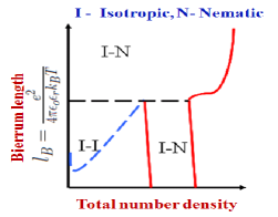
Figure 11: For table of contents use only

REFERENCES

- (1) Cooper, C. L.; Dubin, P. L.; Kayitmazer, A. B.; Turksen, S. Current Opinion in Colloid and Interface Science 2005, 10, 52.
- (2) Thunemann, A. F.; Muller, M.; Dautzenberg, H.; Joanny, J. F. O.; Lowne, H. Polyelectrolyte complexes. In Polyelectrolytes with Defined Molecular Architecture Ii, 2004; Vol. 166; pp 113.
- (3) Belyi, V. A.; Muthukumar, M. Proceedings of the National Academy of Sciences of the United States of America 2006, 103, 17174.
- (4) Hu, T.; Shklovskii, B. I. Physical Review E 2007, 75, 051901.
- (5) Waite, J. H.; Andersen, N. H.; Jewhurst, S.; Sun, C. J. Journal of Adhesion 2005, 81, 297.
- (6) Hong, J. W.; Henme, W. L.; Keller, G. E.; Rinke, M. T.; Bazan, G. C. Advanced Materials 2006, 18, 878.
- (7) Voorn M.J. Advances in Polymer Science - Fortschritte Der Hochpolymeren-Forschung (Springer Berlin / Heidelberg, 1959 ), (1),192-233.
- (8) Veis, A. in Biological Polyelectrolytes(Marcel Dekker Inc., New York, 1970).
- (9) Bakeev,K. N.; Izumrudov, V. A.; Kuchanov, S. I.; Zezin, A. B.; Kabanov, V. A. Macromolecules 1992, 25, 4249.
- (10) Kabanov, A. V.; Bronich, T. K.; Kabanov, V. A.; Yu, K.; Eisenberg,A. Macromolecules 1996, 29, 6797.
- (11) Dautzenberg, H.; Hartmann, J.; Grunewald, S.; Brand, F. Ber. Bunsen-Ges. Phys. Chem. 1996, 100, 1024.
- (12) Pogodina, N. V.; Tsvetkov,N. V. Macromolecules 1997, 30, 4897.
- (13) Dautzenberg, H. Macromolecules 1997, 30,7810.
- (14) Ou, Z. Y.; Muthukumar, M. Journal of Chemical Physics 2006, 124, 11.
- (15) Michaeli, I.; Overbeek, J. T. G.; Voorn, M. J. Journal of Polymer Science 1957, 23, 443.
- (16) Voorn, M. J. Recueil Des Travaux Chimiques Des Pays-Bas-Journal of the Royal Netherlands Chemical Society 1956, 75, 317.
- (17) Voorn, M. J. Recueil Des Travaux Chimiques Des Pays-Bas-Journal of the Royal Netherlands Chemical Society 1956, 75, 405.
- (18) Voorn, M. J. Recueil Des Travaux Chimiques Des Pays-Bas-Journal of the Royal Netherlands Chemical Society 1956, 75, 427.
- (19) Voorn, M. J. Recueil Des Travaux Chimiques Des Pays-Bas-Journal of the Royal Netherlands Chemical Society 1956, 75, 925.
- (20) Voorn, M. J. Recueil Des Travaux Chimiques Des Pays-Bas-Journal of the Royal Netherlands Chemical Society 1956, 75, 1021.
- (21) Borue, V. Y.; Erukhimovich, I. Y. Macromolecules 1990, 23, 3625.
- (22) Kudlay, A.; de la Cruz, M. O. Journal of Chemical Physics 2004, 120, 404.
- (23) Kudlay, A.; Ermoshkin, A. V.; de la Cruz, M. O. Macromolecules 2004, 37, 9231.
- (24) Castelnovo, M.; Joanny, J. F. European Physical Journal E 2001, 6, 377.
- (25) Popov, Y. O.; Lee, J. H.; Fredrickson, G. H. Journal of Polymer Science Part B-Polymer Physics 2007, 45, 3223.
- (26) Lee, J.; Popov, Y. O.; Fredrickson, G. H. Journal of Chemical Physics 2008, 128, 224908.
- (27) Muthukumar, M. Journal of Chemical Physics 1996, 105, 5183.
- (28) de Gennes, P.G.; Prost J. The Physics of Liquid Crystals (Clarendon Press, Oxford, 1993).
- (29) de Gennes, P. G.; Pincus, P.; Velasco, R. M.; Brochard, F. Journal De Physique 1976, 37, 1461.
- (30) Joanny, J. F.; Leibler, L. Journal De Physique 1990, 51, 545.
- (31) Khokhlov, A. R.; Nyrkova, I. A. Macromolecules 1992, 25, 1493.
- (32) Muthukumar, M. Macromolecules 2002, 35, 9142.
- (33) Lee, C. L.; Muthukumar, M. Journal of Chemical Physics 2009, 130, 024904.
- (34) Onsager, L. Annals of the New York Academy of Sciences 1949, 51, 627.
- (35) Stroobants, A.; Lekkerkerker, H. N. W.; Odijk, T. Macromolecules 1986, 19, 2232.
- (36) Chen, S. B.; Koch, D. L. Journal of Chemical Physics 1996, 104, 359.
- (37) Carri, G. A.; Muthukumar, M. Journal of Chemical Physics 1999, 111, 1765.
- (38) Potemkin, II; Limberger, R. E.; Kudlay, A. N.; Khokhlov, A. R. Physical Review E 2002, 66, 011802.
- (39) Potemkin, II; Khokhlov, A. R. Journal of Chemical Physics 2004, 120, 10848.
- (40) Potemkin, II; Oskolkov, N. N.; Khokhlov, A. R.; Reineker, P. Physical Review E 2005, 72, 021804.
- (41) Hoye, J.; Raineri, F. O.; Stell, G.; Routh, J. Journal of Statistical Physics 2003, 110, 835.
- (42) Brenner, S. L.; Parsegia.V.A. Biophysical Journal 1974, 14, 327.
- (43) Doi, M.; Edwards, S.F. The Theory of Polymer Dynamics (Clarendon Press, Oxford, 1986), chapter 10.
- (44) Flory, P. J. Proceedings of the Royal Society of London Series a-Mathematical and Physical Sciences 1956, 234, 73.
- (45) Flory, P. J. Proceedings of the Royal Society of London Series a-Mathematical and Physical Sciences 1956, 234, 60.
- (46) Khokhlov, A. R. Physics Letters A 1978, 68, 135.
- (47) Khokhlov, A. R.; Semenov, A. N. Physica A 1981, 108, 546.
- (48) Dobrynin, A. V.; Rubinstein, M. Progress in Polymer Science 2005, 30, 1049.
- (49) Nishida, K.; Kaji, K.; Kanaya, T. Journal of Chemical Physics 2001, 114, 8671.
- (50) Odijk, T. Journal of Physical Chemistry 1989, 93, 3888.
- (51) Mackintosh, F. C.; Safran, S. A.; Pincus, P. A. Europhysics Letters 1990, 12, 697.
- (52) Franco-Melgar, M.; Haslam, A. J.; Jackson, G. Molecular Physics 2008, 106, 649.
- (53) Manning, G. S. Journal of Chemical Physics 1969, 51, 924.
- (54) Lakatos K. Journal of Statistical Physics 1970,2, 121.
- (55) Lasher, G. Journal of Chemical Physics 1970, 53, 4141.
- (56) Herzfeld, J.; Berger, A. E.; Wingate, J. W. Macromolecules 1984, 17, 1718.
- (57) Press, W.H. et al. Numerical Recipes in C(Cambridge University Press,New York, 1992).
- (58) Kayser, R. F.; Raveche, H. J. Physical Review A 1978, 17, 2067.
- (59) Chandler, D. Introduction to Modern Statistical Mechanics(Oxford University Press, New York, 1987).
- (60) Fisher, M. E.; Levin, Y. Physical Review Letters 1993, 71, 3826.
- (61) Fisher, M. E. Journal of Statistical Physics 1994, 75, 1.
- (62) Fredrickson, G.H. The Equilibrium Theory of Inhomogeneous Polymers (Oxford University Press, New York, 2006).
- (63) Borukhov, I.; Andelman, D.; Borrega, R.; Cloitre M.; Leibler, L.; Orland, H. Journal of Physical Chemistry B 2000, 104 11027.
- (64) Stephen,M.J.; Straley, J.P. Reviews of Modern Physics 1974, 46, 617.
- (65) Parsons, J.D. Physical Review A 1979, 19, 1225.
- (66) Lee, S.D. Journal of Chemical Physics 1987, 87, 4972.
- (67) Diehl, A.; Barbosa, M.C.; Levin, Y. Europhysics Letters 2001, 53, 86.
- (68) Muthukumar, M.; Hua, J.; Kundagrami, A. Journal of Chemical Physics 2010, 132, 084901.
- (69) Wang, Z.W.; Rubinstein, M. Macromolecules 2006, 39, 5897.
- (70) Falkenhagen, H.; Ebeling, W. in Ionic Interactions, edited by S. Petrucci (Academic, New York, 1971), vol. 1.
- (71) Levin, Y. Reports on Progress in Physics 2002, 65, 1577.
- (72) Muthukumar, M. Journal of Chemical Physics 2004, 120, 9343; Kumar, R.; Kundagrami, A.; Muthukumar, M. Macromolecules 2009, 42, 1370.
- (73) Semenov, A.N.; Rubinstein, M. Macromolecules 1998, 31, 1373.