Water in low-mass star-forming regions with Herschel

‘Water In Star-forming regions with Herschel’ (WISH) is a key programme dedicated to studying the role of water and related species during the star-formation process and constraining the physical and chemical properties of young stellar objects. The Heterodyne Instrument for the Far-Infrared (HIFI) on the Herschel Space Observatory observed three deeply embedded protostars in the low-mass star-forming region NGC1333 in several H${}_{2}^{16}$O, H${}_{2}^{18}$O, and CO transitions. Line profiles are resolved for five H${}_{2}^{16}$O transitions in each source, revealing them to be surprisingly complex. The line profiles are decomposed into broad ($>$20 km s^-1), medium-broad ($\sim$5–10 km s^-1), and narrow ($<$5 km s^-1) components. The H${}_{2}^{18}$O emission is only detected in broad 1₁₀–1₀₁ lines ($>$20 km s^-1), indicating that its physical origin is the same as for the broad H${}_{2}^{16}$O component. In one of the sources, IRAS4A, an inverse P Cygni profile is observed, a clear sign of infall in the envelope. From the line profiles alone, it is clear that the bulk of emission arises from shocks, both on small ($\lesssim$1000 AU) and large scales along the outflow cavity walls ($\sim$10 000 AU). The H₂O line profiles are compared to CO line profiles to constrain the H₂O abundance as a function of velocity within these shocked regions. The H₂O/CO abundance ratios are measured to be in the range of $\sim$0.1–1, corresponding to H₂O abundances of $\sim$10^-5–10^-4 with respect to H₂. Approximately 5–10% of the gas is hot enough for all oxygen to be driven into water in warm post-shock gas, mostly at high velocities.

1 Introduction

In the deeply embedded phase of low-mass star formation, it is often only possible to trace the dynamics of gas in a young stellar object (YSO) by analysing resolved emission-line profiles. The various dynamical processes include infall from the surrounding envelope towards the central protostar, molecular outflows caused by jets ejected from the central object, and strong turbulence induced within the inner parts of the envelope by small-scale shocks (Arce et al. 2007, Jørgensen et al. 2007). One of the goals of the Water In Star-forming regions with Herschel (WISH) key programme is to use water as a probe of these processes and determine its abundance in the various components as a function of evolution (van Dishoeck et al. in prep.).

Spectrally resolved observations of the H₂O 1₁₀–1₀₁ line at 557 GHz with ODIN and SWAS towards low-mass star-forming regions have revealed it to be broad, $\sim$20 km s^-1, indicative of an origin in shocks (e.g., Bergin et al. 2003). Within the large beams (2′ and 4′), where both the envelope and the entire outflow are present, outflow emission most likely dominates. Observations and subsequent modelling of the more highly excited H₂O lines with ISO-LWS were unable to distinguish between an origin in shocks or an infalling envelope (e.g., Ceccarelli et al. 1996, Nisini et al. 2002, Maret et al. 2002). Herschel-HIFI has a much higher sensitivity, higher spectral resolution, and smaller beam than previous space-based missions, thus is perfectly suited to addressing this question. Complementary CO data presented by Yıldız et al. (2010) are used to constrain the role of the envelope and determine outflow temperatures and densities.

NGC1333 is a well-studied region of clustered, low-mass star formation at a distance of 235 pc (Hirota et al. 2008). In particular, the three deeply embedded, low-mass class 0 objects IRAS2A, IRAS4A, and IRAS4B have been observed extensively with ground-based submillimetre telescopes (e.g., Jørgensen et al. 2005, Maret et al. 2005) and interferometers (e.g., Di Francesco et al. 2001, Jørgensen et al. 2007). All sources have strong outflows extending over arcmin scales ($>$15 000 AU). Both IRAS4A and 4B consist of multiple protostars (e.g., Choi 2005). Because of the similarities between the three sources in terms of luminosity (20, 5.8, and 3.8 $L_{\odot}$), envelope mass (1.0, 4.5, and 2.9 $M_{\odot}$; Jørgensen et al. 2009) and presumably also age, they provide ideal grounds for comparing YSOs in the same region.

2 Observations and results

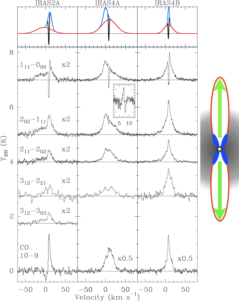
Figure 1: H₂O spectra of the three NGC1333 sources. CO 10–9 is shown for comparison (Yıldız et al. 2010); the CO 10–9 emission in IRAS2A is affected by chopping into outflow material. The top panel shows the decomposition into broad (red), medium (blue), and narrow (black) components. The cartoon illustrates the physical origin of each component. The inset shows a zoom on the inverse P Cygni profile in the H₂O 2₀₂–1₁₁ line of IRAS4A, where the other components have been subtracted; the vertical scale ranges from $-$0.3 to 0.3 K.

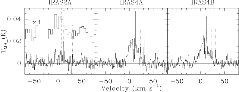
Figure 2: H${}_{2}^{18}$O 1₁₀–1₀₁ spectra of the three NGC1333 sources along with the CH 536 GHz triplet from the lower sideband (dotted lines). Spectra are shown for a channel size of 0.25 km s^-1. The spectrum of IRAS2A has been rebinned to 4 km s^-1 to illustrate the detection of a broad feature. The red line shows the source velocity at $\varv_{\rm LSR}$$\sim$$+$7.5 km s^-1.

Three sources in NGC1333, IRAS2A, IRAS4A, and IRAS4B, were observed with HIFI (de Graauw et al. 2010) on Herschel (Pilbratt et al. 2010) on March 3–15, 2010 in dual beam switch mode in bands 1, 3, 4, and 5 with a nod of 3′. Observations detected several transitions of H₂O and H${}_{2}^{18}$O in the range $E_{\rm u}/k_{\rm B}$$\approx$50–250 K (Table 2 in the online appendix). Diffraction-limited beam sizes were in the range 19–40″ (4500–9500 AU). In general, the calibration is expected to be accurate to $\sim$20% and the pointing to $\sim$2″. Data were reduced with HIPE 3.0. A main-beam efficiency of 0.74 was used throughout. Subsequent analysis was performed in CLASS. The rms was in the range 3–150 mK in 0.5 km s^-1 bins. Linear baselines were subtracted from all spectra, except around 750 GHz (corresponding to the H₂O 2₁₁–2₀₂ transition) where higher-order polynomials are required. A difference in rms was always seen between the H- and V-polarizations, with the rms in the H-polarization being lower. In cases where the difference exceeded 30% and qualitative differences appear in the line profile, the V-polarization was discarded, otherwise the spectra were averaged.

All targeted lines of H${}_{2}^{16}$O were detected and are listed in Table 1 and Fig. 1. The 1₁₀–1₀₁ transition at 557 GHz was not observed before the sources moved out of visibility. The H${}_{2}^{18}$O 1₁₀–1₀₁ line was detected in all sources (Fig. 2), although the detection in IRAS2A was weak ($\sim$5$\sigma$ = 0.13 K km s^-1). This line is superposed on the ground-state CH triplet at 536 GHz, observed in the lower sideband (Fig. 2). Neither the H${}_{2}^{18}$O 1₁₁–0₀₀ nor the 2₀₂–1₁₁ line in IRAS2A is detected down to $\sigma$$<$0.06 K km s^-1.

The H₂O lines exhibit multiple components: a broad emission component (FWHM$>$$20$ km s^-1) sometimes offset from the source velocity ($\varv_{\rm LSR}$=$+$7.2–7.7 km s^-1); a medium-broad emission component (FWHM$\sim$5–10 km s^-1); and a deep, narrow absorption component (FWHM$\sim$2 km s^-1) seen at the source velocity. The individual components are all reproduced well by Gaussian functions. The absorption is only seen in the H₂O 1₁₁–0₀₀ line and is saturated in IRAS2A and IRAS4A. In IRAS4B, the absorption extends below the continuum level, but is not saturated. Furthermore, the IRAS4A spectrum of the 2₀₂–1₁₁ line exhibits an inverse P Cygni profile. The shape of the lines is the same within a source; only the relative contribution between the broad and medium components changes. For example, in IRAS2A the ratio of the peak intensities is $\sim$2, independent of the line, whereas in IRAS4A it ranges from 1 to 2. The H${}_{2}^{18}$O line profiles compare well to the broad component seen in H₂O, i.e., similar FWHM$>$20 km s^-1 and velocity offset. The width is much larger than isotopologue emission of, e.g., C¹⁸O ($\sim$1–2 km s^-1) and is centred on the source velocity (Yıldız et al. 2010). The medium and narrow components are not seen in the H${}_{2}^{18}$O 1₁₀–1₀₁ spectra down to an rms of 2–3 mK in 0.5 km s^-1 bins.

Table 1: H₂O and H${}_{2}^{18}$O emission in the NGC1333 sources.

			Medium			Broad
Source	Transition	rms	$T_{\rm MB}^{\rm peak}$	$\int T_{\rm MB}\leavevmode\nobreak\ {\rm d}\varv$		$T_{\rm MB}^{\rm peak}$	$\int T_{\rm MB}\leavevmode\nobreak\ {\rm d}\varv$
		(mK)	(K)	(K km s-1)		(K)	(K km s-1)
IRAS2A	H2O 111–000	22	0.22	2.7		0.10	4.1
	202–111	25	0.25	2.5		0.12	5.6
	211–202	23	0.16	1.9		0.06	2.7
	312–303	79	0.14	1.5		0.06	2.7
	312–221	52	0.13	1.5		0.08	3.8
	H${}_{2}^{18}$O 110–101	2	…	$<$0.01		0.01	0.14
	111–000	22	…	$<$0.07		…	$<$0.12
	202–111	12	…	$<$0.04		…	$<$0.06
	312–303	19	…	$<$0.06		…	$<$0.10
FWHM (km s-1)			10.7$\pm$0.8			42$\pm$3
$\varv_{\rm LSR}$ (km s-1)			$+$10.7$\pm$0.8			$-$2.3$\pm$3.4
IRAS4A	H2O 111–000	23	0.36	4.9		0.35	15.3
	202–111	24	0.34	3.8		0.45	18.0
	211–202	23	0.14	0.8		0.43	14.0
	312–221	100	0.07	0.4		0.32	13.6
	H${}_{2}^{18}$O 110–101	3	…	$<$0.01		0.02	0.43
	111–000	23	…	$<$0.06		…	$<$0.09
FWHM (km s-1)			11.1$\pm$2.3			37$\pm$4
$\varv_{\rm LSR}$ (km s-1)			$-$0.6$\pm$0.5			$+$8.7$\pm$1.0
IRAS4B	H2O 111–000	29	1.1	5.1		0.54	14.0
	202–111	23	0.63	3.5		0.65	17.6
	211–202	17	0.37	1.8		0.40	10.2
	312–221	150	0.32	1.3		0.76	17.5
	H${}_{2}^{18}$O 110–101	3	…	$<$0.01		0.02	0.43
	111–000	16	…	$<$0.03		…	$<$0.04
FWHM (km s-1)			4.6$\pm$0.5			24$\pm$2
$\varv_{\rm LSR}$ (km s-1)			$+$8.1$\pm$0.3			$+$8.0$\pm$0.5

2

Table 2: Observed H₂O, H${}_{2}^{18}$O and CH transitions.

Transition	$\nu$	$\lambda$	$E_{\rm u}/k_{\rm B}$	$A$	Beam	$t_{\rm int}$
	(GHz)	($\mu$m)	(K)	($10^{-3}$ s-1)	(′′)	(min.)
H2O    111–000	1113.34	269.27	153.4	18.42	19	43.5
202–111	1987.93	303.46	100.8	15.84	22	23.3
211–202	1752.03	398.64	136.9	17.06	29	18.4
312–303	1097.37	273.19	249.4	16.48	20	32.4
312–221	1153.13	259.98	249.4	12.63	19	13.0
H${}_{2}^{18}$O    110–101	1547.68	547.39	160.5	13.59	39	64.3
111–000	1101.70	272.12	152.9	21.27	20	43.5
202–111	1994.68	301.40	100.7	17.05	22	46.7
312–303	1095.16	273.74	289.7	22.12	20	32.4
CH    3/2,2-–1/2,1+	1536.76	558.52	125.8	10.66	39
3/2,1-–1/2,1+	1536.78	558.50	125.8	10.23	39
3/2,1-–1/2,0+	1536.80	558.48	125.8	10.46	39

The upper limits to the H${}_{2}^{18}$O 1₁₁–0₀₀ line are invaluable for estimating upper limits to the optical depth, $\tau$. In the following, the limit on $\tau$ is derived for the integrated intensity; in the line wings, $\tau$ is most likely lower (Yıldız et al. 2010). In the broad component, the limit ranges from 0.4 (IRAS4B) to 2 (IRAS2A), whereas it ranges from 1.1 (IRAS4B) to 2.7 (IRAS2A) for the medium component of the H${}_{2}^{16}$O 1₁₁–0₀₀ line. Performing the same analysis to the upper limit on the H${}_{2}^{18}$O 2₀₂–1₁₁ line observed in IRAS2A, infers an upper limit to the optical depth of H${}_{2}^{16}$O 2₀₂–1₁₁ of 1.5 for the medium component and 1.9 for the broad. Thus it is likely that neither the broad nor the medium components are very optically thick.

3 Discussion

Many physical components in a YSO are directly traced by the line profiles presented here, including the infalling envelope and shocks along the cavity walls. In the following, each component is discussed in detail, and the H₂O abundance is estimated in the various physical components.

3.1 Line profiles

The most prominent feature of all the observed line profiles is their width. All line wings span a range of velocities of $\sim$40–70 km s^-1 at their base. The width alone indicates that the bulk of the H₂O emission originates in shocks along the cavity walls, also called shells, seen traditionally as the standard high-velocity component in CO outflow data, but with broader line-widths due to water enhancement at higher velocities (Sect. 3.2 Bachiller et al. 1990, Santiago-García et al. 2009). The shocks release water from the grains by means of sputtering and in high-temperature regions all free oxygen is driven into water. The shocked regions may be illuminated by FUV radiation originating in the star-disk boundary layer, thus further enhancing the water abundance by means of photodesorption. The broad emission seen in the H${}^{18}_{2}$O 1₁₀–1₀₁ line arises in the same shocks (see cartoon in Fig. 1).

The medium components (FWHM$\sim$5–10 km s^-1) are most likely also caused by shocks, although presumably on a smaller spatial scale and in denser material than the shocks discussed above. For example, the medium component in IRAS2A is seen in other grain-product species such as CH₃OH (Jørgensen et al. 2005, Maret et al. 2005, Fig. 3), where emission arises from a compact region ($<$1″, i.e., $<$250 AU) centred on the source (Jørgensen et al. 2007), and the same is likely true for the medium H₂O component in that source. In interferometric observations of IRAS4A, a small ($\sim$few arcsec) blue-shifted outflow knot of similar width has been identified in, e.g., SiO and SO (Choi 2005, Jørgensen et al. 2007). Small-scale structures exist in the other sources as well, which may produce the medium components.

The H₂O 2₀₂–1₁₁ spectrum of IRAS4A shows an inverse P Cygni profile, a clear sign of infall also detected in other molecular tracers using interferometer observations (Di Francesco et al. 2001, Jørgensen et al. 2007). This infall signature is also tentatively seen in the 1₁₁–0₀₀ line, but here the absorption from the outer envelope dominates and little is left of the blue emission peak. The signature is not seen in higher-excitation lines. The separation of the emission and absorption peaks is $\sim$0.8 km s^-1, whereas it is $\sim$1.5 km s^-1 in the observations of Di Francesco et al. (2001) and larger in the observations by Jørgensen et al. (2007), indicating that the infall observed in H₂O 2₀₂–1₁₁ takes place over larger spatial scales.

The passively heated envelope is seen in ground-based observations of high-density tracers to produce narrow emission, $<$3 km s^-1, which may be self-absorbed (Fig. 3). For water, this type of emission is not seen in any of the sources; the medium component is broader by a factor of 2–3 with respect to what is expected from the envelope. The absorption seen in all three sources is attributed to cold gas in the outer parts of the envelope. Using interferometric observations, Jørgensen & van Dishoeck (2010) detected compact, narrow ($\sim$1 km s^-1) emission in the H${}^{18}_{2}$O 3₁₃–2₂₀ line in IRAS4B possibly originating in the circumstellar disk. Scaling the observed emission to the transitions observed here by assuming $T_{\rm rot}$=170 K (Watson et al. 2007), the expected emission is typically less than 10% of the rms for any given transition. Hence, when extrapolated to the disks surrounding IRAS2A and 4A, the disk contribution to the H₂O emission probed by HIFI is negligible. The H₂O excitation temperature of the broad component is 220$\pm$30 K, comparable to that found by Watson et al. (2007), but the inferred column density is a factor of 100 higher. Thus, the mid-infrared lines seen by Watson et al. may come from the same broad outflowing gas found by HIFI, provided the mid-infrared lines experience a factor of 100 more extinction.

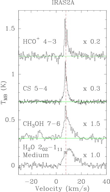
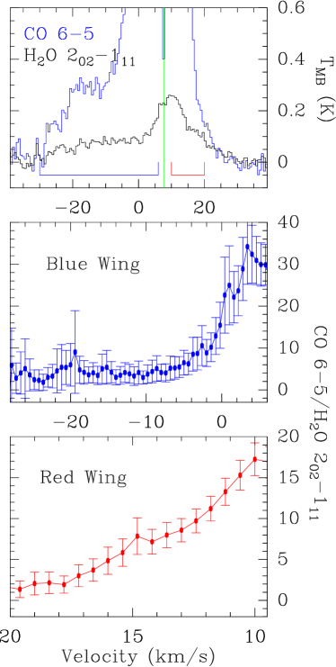
Figure 3: Left. Comparison between the medium component in IRAS2A and other species observed with ground-based telescopes. The broad component has been subtracted for easy comparison. The vertical red line indicates the source velocity at $+$7.7 km s^-1. Right. Comparison between H₂O 2₀₂–1₁₁ and CO 6–5 obtained with APEX-CHAMP⁺, and emission ratios for the blue- and red-shifted outflow lobes.

3.2 Abundances

3.2.1 Shocks: H₂O/CO

The observed broad components are compared directly with HIFI observations of CO 10–9 (Yıldız et al. 2010), because the width and position of the lines are similar and they were obtained using approximately the same beamsize (22″ versus 19″). The exception is for IRAS2A, where the blue line wing is not observed. The advantage is that no detailed models are required to account for the H₂O/CO abundance, as long as the lines are optically thin, in particular the emission from the wings. The abundance ratio is estimated for various temperatures by using the RADEX escape probability code (van der Tak et al. 2007). The density is assumed to be 10⁵ cm^-3, appropriate for the large-scale core. If the emission is optically thin, the abundance ratio scales linearly with density resulting in the same line ratio corresponding to a higher abundance ratio. There is little variation in the predicted ratio for $T$$>$150 K, the typical temperature inferred by Yıldız et al. (2010). The line ratios and abundance ratios are listed as a function of velocity in Table 3 in the online appendix.

The abundance ratio increases with increasing velocity from H₂O/CO of $\sim$0.2 near the line centre to H₂O/CO$\gtrsim$1 in the line wings of all sources for velocity offsets larger than 15 km s^-1 with respect to that of the source (Fig. 3). Assuming that the CO abundance is 10^-4, the H₂O abundances are in the range of $\sim$10^-5–10^-4. Only at high velocities is the temperature high enough for oxygen to be driven into water by means of the neutral-neutral reaction O + H₂ $\rightarrow$ OH + H; OH + H₂ $\rightarrow$ H₂O. The same result was found in the massive outflow in Orion-KL (Franklin et al. 2008), where less than 1% of the gas in the outflow experiences this high-temperature phase. The fraction of gas for which the H₂O/CO abundance is $>$1 is $\sim$5–10% for the sources observed here.

For IRAS2A, a deep spectrum of CO 6–5 obtained with CHAMP⁺ on APEX simultaneously with observations of HDO 1₁₁–0₀₀ (Liu et al. in prep.) shows the same morphology in terms of a broad and medium component (Fig. 3). Furthermore, the velocity offset and FWHM are the same as for H₂O suggesting that the line profiles are not unique to H₂O, although the broad component is far more prominent in H₂O. The ratio of peak intensities for the two components is $\sim$2–3 in H₂O versus 10 in CO 6–5. Analysing the abundance ratio as a function of temperature shows that H₂O/CO$\sim$0.1–1 for $T$$>$150 K (Table 3), consistent with what is found for CO 10–9.

3.2.2 Envelope

The simplest way to constrain the H₂O abundance in the outer envelope is with calculations using RADEX on the narrow absorption in the 1₁₁–0₀₀ line. The absorption is optically thick – in particular for IRAS2A and 4A, where the feature is saturated – which requires a para-H₂O column density of $>$10¹³ cm^-2 if one assumes typical values for $T$ and $n({\rm H}_{2})$ of 15 K and 10⁵ cm^-3. With a pencil-beam H₂ column of $\sim$$10^{23}$ cm^-2 (Jørgensen et al. 2002), the total H₂O abundance in the outer envelope is $\gtrsim$10^-10.

For IRAS2A and 4A, the H₂O abundance was further constrained using radiative transfer models. The setup is a spherical envelope with density and temperature profiles constrained from continuum data (Jørgensen et al. 2009), an infall velocity profile $\varv=(2\,{\rm km}\,{\rm s}^{-1})(r/r_{\rm in})^{-1/2}$, and a Doppler parameter $b=0.8$ km s^-1. Line fluxes were computed with the new radiative transfer code LIME (Brinch & Hogerheijde subm.). The models constrained the abundance of water in the outer envelope to be $\sim$10^-8. Lower values are insufficient to obtain saturated absorption in the 1₁₁–0₀₀ line, and $\sim$10^-8 is the highest abundance where the resulting narrow emission can be hidden in the observed higher-excitation H₂O lines. The models predict that the H₂O emission from the warm inner envelope ($r$$\lesssim$100 AU) is optically thick, hence no constraints can be obtained from the H₂O spectra on the inner abundance. However, the lack of narrow H${}_{2}^{18}$O emission infers an upper limit on the H₂O abundance of $\sim$10^-5 (Visser et al. in prep.).

4 Conclusions

These observations represent one of the first steps towards understanding the formation and excitation of water in low-mass star-forming regions by means of resolved line profiles. The three sources have remarkably similar line profiles. Both the H${}_{2}^{16}$O and H${}_{2}^{18}$O lines are very broad, indicating that the bulk of the emission originates in shocked gas. The broad emission also highlights that water is a far more reliable dynamical tracer than, e.g., CO. Comparing C¹⁸O to H${}^{18}_{2}$O emission and line profiles indicates that the H₂O/CO abundance is high in outflows and low in the envelope. Additional modelling of the emission, should be able to constrain the total amount of water in the envelope and outflowing gas, thus test the high-temperature gas-phase chemistry models for the origin of water. This will be performed for a total sample of the 29 low-mass YSOs to be observed within the WISH key programme.

3

Table 3: CO 6–5 and CO 10–9/H₂O 2₀₂–1₁₁ line ratios in 5 km s^-1 intervals and corresponding abundance ratio for $T$$>$150 K and $n$=10⁵ cm^-3.

d$\varv_{\rm LSR}$	IRAS2A				IRAS4A		IRAS4B
(km s-1)	CO 6–5/	$x$(H2O)/	CO 10–9/	$x$(H2O)/	CO 10–9/	$x$(H2O)/	CO 10–9/	$x$(H2O)/
	H2O 202–111	$x$(CO)	H2O 202–111	$x$(CO)	H2O 202–111	$x$(CO)	H2O 202–111	$x$(CO)
$-$20 – $-$15	5.0	0.34	…	…	0.8	1.11	…	…
$-$15 – $-$10	3.8	0.45	…	…	2.0	0.43	0.9	1.00
$-$10 – $-$5	4.6	0.37	…	…	2.8	0.31	1.4	0.64
$-$5 – 0	9.3	0.18	…	…	2.4	0.36	1.7	0.50
0 – 5	26.6	0.06	…	…	2.9	0.29	2.3	0.37
5 – 10	17.0	0.10	3.4	0.26	3.9	0.22	2.9	0.29
10 – 15	11.1	0.15	3.2	0.27	3.3	0.26	2.1	0.42
15 – 20	3.5	0.48	0.9	1.00	2.4	0.36	1.6	0.53
20 – 25	1.4	1.25	0.4	2.00	1.0	0.83	1.1	0.77
25 – 30	…	…	…	…	0.8	1.11	0.5	1.67
30 – 35	0.9	2.00	…	…	…	…	0.9	1.00

References

- Arce et al. (2007) Arce, H. G., Shepherd, D., Gueth, F., et al. 2007, in Protostars and Planets V, ed. B. Reipurth, D. Jewitt, & K. Keil, 245–260
- Bachiller et al. (1990) Bachiller, R., Martin-Pintado, J., Tafalla, M., Cernicharo, J., & Lazareff, B. 1990, A&A, 231, 174
- Bergin et al. (2003) Bergin, E. A., Kaufman, M. J., Melnick, G. J., Snell, R. L., & Howe, J. E. 2003, ApJ, 582, 830
- Ceccarelli et al. (1996) Ceccarelli, C., Hollenbach, D. J., & Tielens, A. G. G. M. 1996, ApJ, 471, 400
- Choi (2005) Choi, M. 2005, ApJ, 630, 976
- de Graauw et al. (2010) de Graauw et al. 2010, A&A, 518, L6
- Di Francesco et al. (2001) Di Francesco, J., Myers, P. C., Wilner, D. J., Ohashi, N., & Mardones, D. 2001, ApJ, 562, 770
- Franklin et al. (2008) Franklin, J., Snell, R. L., Kaufman, M. J., et al. 2008, ApJ, 674, 1015
- Hirota et al. (2008) Hirota, T., Bushimata, T., Choi, Y. K., et al. 2008, PASJ, 60, 37
- Jørgensen et al. (2007) Jørgensen, J. K., Bourke, T. L., Myers, P. C., et al. 2007, ApJ, 659, 479
- Jørgensen et al. (2002) Jørgensen, J. K., Schöier, F. L., & van Dishoeck, E. F. 2002, A&A, 389, 908
- Jørgensen et al. (2005) Jørgensen, J. K., Schöier, F. L., & van Dishoeck, E. F. 2005, A&A, 437, 501
- Jørgensen & van Dishoeck (2010) Jørgensen, J. K. & van Dishoeck, E. F. 2010, ApJ, 710, L72
- Jørgensen et al. (2009) Jørgensen, J. K., van Dishoeck, E. F., Visser, R., et al. 2009, A&A, 507, 861
- Maret et al. (2002) Maret, S., Ceccarelli, C., Caux, E., Tielens, A. G. G. M., & Castets, A. 2002, A&A, 395, 573
- Maret et al. (2005) Maret, S., Ceccarelli, C., Tielens, A. G. G. M., et al. 2005, A&A, 442, 527
- Nisini et al. (2002) Nisini, B., Giannini, T., & Lorenzetti, D. 2002, ApJ, 574, 246
- Pickett et al. (1998) Pickett, H. M., Poynter, I. R. L., Cohen, E. A., et al. 1998, Journal of Quantitative Spectroscopy and Radiative Transfer, 60, 883
- Pilbratt et al. (2010) Pilbratt et al. 2010, A&A, 518, L1
- Santiago-García et al. (2009) Santiago-García, J., Tafalla, M., Johnstone, D., & Bachiller, R. 2009, A&A, 495, 169
- van der Tak et al. (2007) van der Tak, F. F. S., Black, J. H., Schöier, F. L., Jansen, D. J., & van Dishoeck, E. F. 2007, A&A, 468, 627
- Watson et al. (2007) Watson, D. M., Bohac, C. J., Hull, C., et al. 2007, Nature, 448, 1026
- Yıldız et al. (2010) Yıldız et al. 2010, A&A, this volume