Theoretical Perspectives on Protein Folding

Abstract

Understanding how monomeric proteins fold under in vitro conditions is crucial to describing their functions in the cellular context. Significant advances both in theory and experiments have resulted in a conceptual framework for describing the folding mechanisms of globular proteins. The experimental data and theoretical methods have revealed the multifaceted character of proteins. Proteins exhibit universal features that can be determined using only the number of amino acid residues ($N$) and polymer concepts. The sizes of proteins in the denatured and folded states, cooperativity of the folding transition, dispersions in the melting temperatures at the residue level, and time scales of folding are to a large extent determined by $N$. The consequences of finite $N$ especially on how individual residues order upon folding depends on the topology of the folded states. Such intricate details can be predicted using the Molecular Transfer Model that combines simulations with measured transfer free energies of protein building blocks from water to the desired concentration of the denaturant. By watching one molecule fold at a time, using single molecule methods, the validity of the theoretically anticipated heterogeneity in the folding routes, and the $N$-dependent time scales for the three stages in the approach to the native state have been established. Despite the successes of theory, of which only a few examples are documented here, we conclude that much remains to be done to solve the “protein folding problem” in the broadest sense.

1 INTRODUCTION

The quest to solve the protein folding problem in quantitative detail, which is surely only the first step in describing the functions of proteins in the cellular context, has led to great advances on both experimental and theoretical fronts [85, 92, 38, 144, 130, 125, 127, 30, 105, 28, 117, 6, 114, 35, 141, 5, 26, 27, 8, 43]. In the process our vision of the scope of the protein folding problem has greatly expanded. The determination of protein structures by X-ray crystallography [70] and the demonstration that proteins can be reversibly folded following denaturation [3] ushered in two research fields. The first is the prediction of the three dimensional structures given the amino acid sequence [11, 97], and the second is to describe the folding kinetics [114, 106, 125]. Another line of inquiry in the protein folding field opened with the discovery that certain proteins require molecular chaperones to reach the folded state [46, 140, 58, 128]. More recently, the realization that protein misfolding, which is linked to a number of diseases, has provided additional wrinkles to the already complicated protein folding problem [21, 116, 126, 36]. Although known for a long time it is becoming more widely appreciated that the restrictions in the conformational space in the tight cellular compartments might have significant effect on all biological processes including protein folding [20, 142]. In all these situations the protein folding problem is at the center stage. The solution to this problem requires a variety of experimental, theoretical and computational tools. Advances in all these fronts have given us hope that many aspects of, perhaps the “simplest” of the protein folding problems, namely, how single domain globular proteins navigate the large dimensional potentially rugged free energy surface en route to the native structure are under theoretical control.

Much of our understanding of the folding mechanisms comes from studies of proteins that are described using the two-state approximation in which only the unfolded and folded states are thought to be significantly populated. However, proteins are finite size branched polymers in which the native structure is only marginally stabilized by a number of relatively weak ($\sim O(k_{B}T)$) interactions. From a microscopic point of view the unfolded state and even the folded state should be viewed as an ensemble of structures. Of course, under folding conditions the fluctuations in the native state are less than in the unfolded state. In this picture rather than viewing protein folding as a unimolecular reaction ($U\leftrightarrow F$ where $U$ and $F$ being the unfolded and folded states respectively) one should think of the folding process as the interconversion of the conformations in the Denatured State Ensemble (DSE) to the ensemble of structures in the Native Basin of Attraction (NBA). The description of the folding process in terms of distribution functions necessarily means that appropriate tools in statistical mechanics together with concepts in polymer physics [23, 42, 31, 49] are required to understand the self-organization of proteins, and for that matter RNA [125].

Here, we provide theoretical perspectives on the thermodynamics and kinetics of protein folding of small single domain proteins with an eye towards understanding and anticipating the results of single molecule experiments. The outcome of these experiments are most ideally suited to reveal the description based on changes in distribution functions that characterize the conformations of proteins as the external conditions are varied. Other complementary theoretical viewpoints on the folding of single domain proteins have been described by several researchers [106, 117, 28, 118, 120].

2 UNIVERSALITY IN PROTEIN FOLDING THERMODYNAMICS

The natural variables that should control the generic behavior of protein folding are the length ($N$) of the protein, topology of the native structure [5], symmetry of the native state [79, 135], and the characteristic temperatures that give rise to the distinct “phases” that a protein adopts as the external conditions (such as temperature $T$ or denaturant concentration ([C])) are altered [123]. In terms of these variables, several universal features of the folding process can be derived, which. shows that certain aspects of protein folding can be understood using concepts developed in polymer physics [23, 42, 31, 49].

2.1 Protein Size Depends on Length

Under strongly denaturing conditions proteins ought to exhibit random coil characteristics. If this were the case, then based on Flory theory [42], the radius of gyration ($R_{G}$) of proteins in the unfolded state must scale as $R_{G}^{D}\approx a_{D}N^{\nu}$ where $a_{D}$ is a characteristic Kuhn length, $N$ is the number of amino acid residues, and $\nu\approx 0.6$. Analysis of experimental data indeed confirms the Flory prediction (Fig.1a) [80], which holds good for homopolymers in good solvents. Because folded proteins are maximally compact the native states should obey $R_{G}^{N}\approx a_{N}N^{\nu}$ with $\nu=1/3$. Explicit calculations of $R_{G}$ for a large number of proteins in the Protein Data Bank (PDB) show that the expected scaling is obeyed for the folded states as well (Fig.1b) [29].

2.2 Characteristic Phases

Proteins are finite-sized systems that undergo phase changes as the quality of solvent is decreased. As the $T$ ([C]) is lowered to the collapse temperature $T_{\theta}$ ([C]_θ), which decreases the solvent quality, a transition from an expanded to an ensemble of compact structures must take place. The collapse transition can be either first or second order [23], depending on the nature of the solvent-mediated interactions. In a protein there are additional energy scales that render a few of the exponentially large number of conformations lower in free energy than the rest. These minimum energy compact structures (MECS) direct the folding process [17]. When the temperature is lowered to the folding transition temperature $T_{F}$, a transition to the folded native structure takes place. These general arguments suggest that there are minimally three phases for a protein as $T$ or [C] is varied. They are the unfolded ($U$) states, an ensemble of intermediate ($I$) structurally heterogeneous compact states, and the native state.

An order parameter that distinguishes the $U$ and $I$ states is the monomer density, $\rho=N/R_{G}^{3}$. It follows from the differences in the size dependence of $R_{G}$ in the $U$ and $I$ states with $N$ (Fig. 1) that $\rho\approx 0$ in the $U$ phase while $\rho\approx O(1)$ in the $I$ and the NBA. The structural overlap function ($\chi$), which measures the similarity to the native structure, is necessary to differentiate between the $I$ and the conformations in the NBA. The collapse temperature may be estimated from the changes in the $R_{G}$ values of the unfolded state as $T$ is lowered while $T_{F}$ may be calculated from $\Delta\chi=\langle\chi^{2}\rangle-\langle\chi\rangle^{2}$, the fluctuations in $\chi$.

2.3 Scaling of Folding Cooperativity with $N$ is Universal

A hallmark of the folding transition of small single domain proteins is that it is remarkably cooperative (Fig.2). The marginal stability criterion can be used to infer the $N$-dependent growth of a dimensionless measure of cooperativity $\Omega_{c}=\frac{T_{F}^{2}}{\Delta T}|\frac{df_{NBA}}{dT}|_{T=T_{F}}$ [74], where $\Delta T$ is the full width at half maximum of $|\frac{df_{NBA}}{dT}|$, in a way that reflects both the finite-size of proteins and the global characteristics of the denatured states.

The dependence of $\Omega_{c}$ on $N$ is derived using the following arguments [88]. (i) $\Delta\chi$ is analogous to susceptibility in magnetic systems and hence can be written as $\Delta\chi=T|d\langle\chi\rangle/dh|$, where $h$ is an ordering field conjugate to $\chi$. Because $\Delta\chi$ is dimensionless, we expect that the ordering field $h\sim T$. Thus, $T|d\langle\chi\rangle/dT|\sim T|df_{NBA}/dT|$ plays the role of susceptibility in magnetic systems. (ii) Efficient folding in apparent two-state folders implies $T_{F}\approx T_{\theta}$ [16] (or equivalently $C_{\theta}\approx C_{F}$ [74] when folding is triggered by denaturants). Therefore, the critical exponents that control the behavior of the polypeptide chain at $T_{\theta}$ must control the thermodynamics of the folding phase transition. At $T\approx T_{\theta}\approx T_{F}$ the Flory radius $R_{G}\sim\Delta T^{-\nu}\sim N^{\nu}$. Thus, $\Delta T\sim N^{-1}$ (Fig.2b). Because of the analogy to magnetic susceptibility, we expect $T|d\langle\chi\rangle/dT|\sim N^{\gamma}$. Using these results we obtain $\Omega_{c}\approx N^{\zeta}$ where $\zeta=1+\gamma$, which follows from the hypothesis that $T_{F}\approx T_{\theta}$. The fifth order $\epsilon$ expansion for polymers using $n$-component field theory with $n\rightarrow 0$ gives $\gamma=1.22$, giving $\zeta=2.22$ [72].

The linear fit to the log-log plot of the dependence of $\Omega_{c}$ for proteins shows that $\zeta=2.17\pm 0.09$ for proteins (Fig.2c). The remarkable finding that expresses cooperativity in terms of $N$ and $\zeta$ gives further credence to the proposal that efficient folding is achieved if sequences are poised to have $T_{F}\approx T_{\theta}$ [16, 73].

3 GENERAL PRINCIPLES THAT GOVERN FOLDING KINETICS

A few general conclusions about how proteins access the NBA may be drawn by visualizing the folding process in terms of navigation of a large dimensional folding landscape (Fig. 3a). Dynamics of random heteropolymers have shown that their energy landscapes are far too rugged to be explored [12] on typical folding times (on the order of milliseconds). Therefore, the energy landscape of many evolved proteins must be smooth (or funnel-like [84, 106, 28]) i.e., the gradient of the energy landscape towards the NBA is “large” enough that the biomolecule does not pause in Competing Basins of Attraction (CBAs) for long times during the folding process. Because of energetic and topological frustration the folding landscapes of even highly evolved proteins is rugged on length scales smaller than $R_{G}$ [130, 63]. In the folded state, the hydrophobic residues are usually sequestered in the interior while polar and charged residues are better accommodated on the protein surface. Often these conflicting requirements cannot be simultaneously satisfied and hence proteins can be energetically “frustrated” [50, 22]. If the packing of locally formed structures is in conflict with the global fold then the polypeptide chain is topologically frustrated. Thus, the energy landscape rugged on length scales that are larger than those in which secondary structures ($\approx(1-2)$ $nm$) form even if folding can be globally described using the two-state approximation.

There are several implications of the funnel-like and rugged landscapes for folding kinetics (Fig.3a). (i) Folding pathways are diverse. The precise folding trajectory that a given molecule follows depends on the initial conformation and the location in the landscape from which folding commences. (ii) If the scale of ruggedness is small compared to $k_{B}T$ ($k_{B}$ is the Boltzmann constant) then trapping in CBAs for long times is unlikely, and hence folding follows exponential kinetics. (iii) On the other hand if the space of CBAs is large then a substantial fraction of molecules can be kinetically trapped in one or more of the CBAs. If the time scale of interconversion between the conformations in the CBAs and the NBA is long then the global folding would occur through well-populated intermediates.

3.1 Multiple Folding Nuclei (MFN) Model

Theoretical studies [50, 124, 13, 1] and some experiments [39, 65] suggest that efficient folding of these proteins is consistent with a NC mechanism according to which the rate limiting step involves the formation of one of the folding nuclei. Because the formation of the folding nucleus and the collapse of the chain are nearly synchronous, we referred to this process as the NC mechanism.

Simple theories have been proposed to estimate the free energy cost of producing a structure that contains a critical number $N_{R}^{*}$ residues whose formation drives the structure to the native state [136, 50, 19]. In the simple NC picture the barrier to folding occurs because the formation of contacts (native or non-native) involving the $N_{R}^{*}$ residues, while enthalpically favorable, is opposed by surface tension. In addition, formation of non-native interactions in the transition state also creates strain in the structures representing the critical nuclei. Using a version of the nucleation theory and structure-based thermodynamic data, we showed the average size of the most probable nucleus $N_{R}^{*}$, for single domain proteins, is between 15-30 residues [19].

Simulations using lattice and off-lattice established the validity of the MFN model according to which certain contacts (mostly native) in the conformations in Transition State Ensemble (TSE) form with substantial probability ($>0.5$). An illustration (Fig.3c) is given from a study of the lattice model with side chains [77] in which the distribution of native contacts ($P_{N}(q)$) shows that about 45% of the total number of native contacts have high probability of forming in the TSE and none of them form with unit probability. Although important [86], very few non-native contacts have high probability of forming at the transition state.

3.2 Kinetic Partitioning Mechanism (KPM)

When the scale of roughness far exceeds $k_{B}T$ so that the folding landscape partitions into a number of distinct CBAs that are separated from each other and the NBA by discernible free energy barriers (Fig.3a) then folding is best described by the KPM. A fraction $\Phi$ of molecules can reach the NBA rapidly Fig.3a). The remaining fraction, $1-\Phi$, is trapped in a manifold of discrete intermediates. Since the transitions from the CBAs to the NBA involve partial unfolding, crossing of the free energy barriers for this class of molecules is slow. The KPM explains the not only the folding of complex structured proteins but also counterion-induced assembly of RNA especially Tetrahymena ribozyme [125]. For RNA and large proteins $\Phi\approx(0.05-0.2)$ [125, 71, 107]. The KPM is also the basis of the Iterative Annealing Mechanism [132, 122].

3.3 Three Stage Multipathway Kinetics and the Role of $N$

The time scales associated with distinct routes followed by the unfolded molecules (Fig.3) can be approximately estimated using $N$. For the case when $\Phi\approx 0$, the folding time $\tau_{F}\sim\tau_{0}N^{2+\theta}$ where the $1.8\leq\theta\leq 2.2$ [123]. The theoretically predicted power law dependence was validated in lattice model simulations in a subsequent study [51].

Simulations using lattice and off-lattice models showed that the molecules that follow the slow track reach the native state in three stages (Fig.3b) [16, 50, 123].

Non-specific Collapse: In the first stage the polypeptide chain collapses to an ensemble of compact conformations driven by the hydrophobic forces. The conformations even at this stage might have fluctuating secondary and tertiary structures. By adopting the kinetics of coil-globule formation in hompolymers it was shown that the time scale for non-specific collapse $\tau_{nc}\approx\tau_{c0}N^{2}$.

Kinetic Ordering: In the second phase the polypeptide chain effectively discriminates between the exponentially large number of compact conformations to attain a large fraction of native-like contacts. At the end of this stage the molecule finds one of the basins corresponding to the MECS. Using an analogy to reptation in polymers we suggested that the time associated with this stage is $\tau_{KO}\sim\tau_{KO0}N^{3}$ [17].

All or None: The final stage of folding corresponds to activated transitions from one of the MECS to the native state. A detailed analysis of several independent trajectories for both lattice and off-lattice simulations suggest that there are multiple pathways that lead to the structures found at the end of the second stage. There are relatively few paths that connect the native state and the numerous native-like conformations located at the end of the second stage (Fig.3b).

In majority of ensemble experiments only the third folding stage is measured. The folding time $\tau_{F}\approx\tau_{0}\exp(\Delta F^{\ddagger}/k_{B}T)$ where the barrier height $\Delta F^{\ddagger}\approx\sqrt{N}$. Others have argued that $\Delta F^{\ddagger}\approx N^{2/3}$ [136, 40]. The limited range of $N$ for which data are available makes it difficult to determine the exponent unambiguously. However, correlation of the stability of the folded states [123] expressed as $Z$-score ($\propto\sqrt{N}$) with folding time [75] shows that $\sqrt{N}$ scaling [98, 2] is generic (Fig. 3d).

4 MOVING FORWARD : NEW DEVELOPMENTS

Theoretical framework and simulations (especially using a variety of coarse-grained models [55, 22, 47, 48, 101, 69, 68, 57]) have been instrumental in making testable predictions for folding of a number of proteins. For example, by combining structural analyses of a number of SH3 domains using polymer theory, and off-latice simulations we showed that the stiffness of the distal loop is the reason for the observation of polarized transition state in src SH3 and $\alpha$-spectrin SH3 [78]. The theoretical prediction was subsequently validated by Serrano and coworkers [121]. This and other successful applications that combine simulations and experiments legitimately show that, from a broad perspective, how proteins fold is no longer as daunting a problem as it once seemed.

On the experimental front impressive advances, especially using single molecule FRET (smFRET) [100, 119, 109, 54, 110, 14, 82, 90, 115] and Single Molecule Force spectroscopy (SMFS) [139, 45, 37, 24] pose new challenges that demand more quantitative predictions. Although still in their infancy, single molecule experiments have established the need to describe folding in terms of shifts in the distribution functions of the properties of the proteins as the conditions are changed, rather than using the more traditional well-defined pathway approach. New models that not only make precise connections to experiments but also produce far reaching predictions are needed in order to take the next leap in the theory of protein folding.

5 MOLECULAR TRANSFER MODEL (MTM) : CONNECTING THEORY AND EXPERIMENT

Almost all of the computational studies to date have been done using temperature to trigger folding and unfolding, while protein stability and kinetics in a majority of the experiments are probed using chemical denaturants. A substantial conceptual advance to narrow the gap between experiments and computations was made with the introduction of the MTM theory [102, 103]. The goal of the MTM is to combine simulations at condition A, and reweighting the protein conformational ensemble appropriately such that the behavior of the protein under solution condition B($\equiv\{T_{B},pH_{B},[C_{B}]\}$) can be accurately predicted without running additional simulations at B. By using the partition function $Z(A)=\sum_{i}e^{-\beta_{A}E_{i}(A)}$ in condition A ($\beta_{A}=(k_{B}T_{A})^{-1}$ and $E_{i}(A)$ is the potential energy of the $i^{th}$ microstate), and the free energy cost of transferring $i$ from A to B (denoted $G_{tr,i}(A\rightarrow B)$) the partition function $Z(B)=\sum_{i}e^{-\beta_{B}(E_{i}(A)+G_{tr,i}(A\rightarrow B))}$ in condition B can be calculated (Fig.4a).

5.1 Applications to Protein L and Cold Shock Protein

In the applications of MTM theory to date we have used the $C_{\alpha}$-side chain model ($C_{\alpha}-SCM$) for proteins so that accurate calculation of $Z(A)$ can be made. The phenomenological Transfer Model [10], which accurately predicts $m$-values for a large number of proteins (Fig.4b), is used to compute $G_{tr,i}(A\rightarrow B)$ for each protein conformation using the measured [C]-dependent transfer free energies of amino side chains and backbone from water to a [C]-molar solution of denaturant or osmolyte.

The success of the MTM is evident by comparing the results of simulations with the GdmCl-dependent changes in $f_{NBA}$ and FRET efficienty ($\langle E\rangle$) for protein L and CspTm cold shock proteins (Fig.4c and 4d). Notwithstanding the discrepancies among different experiments, the predictions of $\langle E\rangle$ as a function of GdmCl concentration are in excellent agreement with experiments (Fig.4d). The calculations in Fig.4 are the first to show that quantitative agreement between theory and experiment can be obtained, thus setting the stage for extracting [C]-dependent structural changes that occur during the folding process.

5.2 Characterization of the Denatured State Ensemble

How does the DSE change as [C] decreases? A total picture of the folding process requires knowledge of the distributions of various properties of interest, namely, secondary and tertiary structure contents and the end-to-end distance $R_{ee}$ as [C] changes. The MTM simulations reveal a number of surprising results regarding the DSE properties of globular proteins in general and protein L and CspTm in particular. (i) Certain properties ($R_{G}$ for example) may indicate that high denaturant concentration is a good solvent for proteins (Fig.1a) while others give a more nuanced picture of the DSE properties [103]. If high [C] is a good solvent then from polymer theory it can be shown that the end-to-end distribution function $P_{T}(x)\sim x^{\delta}\exp{(-x^{\frac{1}{1-\nu}})}$, where $x=R_{ee}/\langle R_{ee}\rangle$ ($\langle R_{ee}\rangle$ is the average end-to-end distance) should be universal with the exponent $\delta\approx 0.3$ in three dimensions. Although the scaling of $R_{G}^{D}\sim N^{\nu}$ of the DSE with $\nu\approx 0.6$ (Fig.1a) suggests that the DSE can be pictured as a random coil, the simulated $P(x)$ for protein L deviates from $P_{T}(x)$, which shows that even at high GdmCl remnants of structure must persist (Fig.5a). (ii) An important finding in smFRET experiments is that the statistical characteristics of the DSE changes substantially as [C]$<C_{m}$, the midpoint concentration at which the populations of the unfolded and folded structure are equal. For a number of proteins, including protein L and CspTm, there is a collapse transition predicted theoretically (Fig.5b) and demonstrated in smFRET [114, 119]. For $[C]>>C_{m}$ only moderate changes in $R_{G}^{D}$ are observed while larger changes occur as $[C]<C_{m}$ (Fig.5b). Concomitant with the equilibrium collapse, the fraction of residual structure increases, with the largest increase occurring below $C_{m}$ [103]. Thus, the DSE becomes compact and native-like as [C] decreases, which shows that the collapse process should be a generic step during the folding process (Fig.5b).

5.3 Constancy of $m$-values and Protein Collapse

A number of the smFRET experiments show that the DSE undergoes a continuous collapse as [C] decreases [143], which implies that the accessible surface area must also change with decreasing denaturant concentration. These observations would suggest that the stability of the native state must be a non-linear function of [C] even when $[C]>C_{m}$, which contradicts a large number of measurements, which show that free energy chages linearly with [C]. The apparent contradiction was addressed using simulations and theory both of which emphasize the polymer nature of proteins [102, 143]. Explicit simulations of protein L showed that the constancy of $m$-value (= $d\Delta G_{ND}/d[C]$ where $\Delta G_{ND}$ is the stability of the NBA with respect to DSE) arises because [C]-dependent surface area of the backbone that makes the largest contribution to $m$ does not change appreciably when $[C]>C_{m}$. In an alternative approach to the TM model, Ziv and Haran [143] used polymer theory and experimental data on 12 proteins and showed that the $m$-value can be expressed in terms of a [C]-dependent interaction energy and the volume fraction of the protein in the expanded state (Fig. 5f).

The continuous nature of the collapse transition has also been unambiguously demonstrated in a series of studies by Udgaonkar and coworkers [67, 133, 83] who have shown that the collapse process (both thermodynamically and kinetically) is a continuous process, and the description of folding as a two-state transition clearly obscures the hidden complexity.

5.4 Transition Midpoints are Residue-Dependent

The obsession with the two-state description of the folding transition as [C] (or $T$) is changed, using only simple order parameters (see below), has led to molecular explanations of the origin of cooperativity without examination of the consequences of finite size effects. For instance, the van’t Hoff criterion (coincidence of calorimetric enthalpy and the one extracted from fitting $f_{NBA(i)}$ to two states) and the superposition of denaturation curves generated using various probes such as SAXS, CD, and FRET are often used to assert that protein folding can be described using only two states. However, these descriptions, which use only a limited set of order parameters, are not adequate for fully describing the folding transition.

The order parameter theory for first and second order phase transitions is most useful when the decrease in symmetry from a disordered to an ordered phase can be described using simple physically transparent variables. For example, magnetization and Fourier components of the density are appropriate order parameters for spin systems (second order transition) and the liquid to solid transition (first order transition) [108], respectively. In contrast, devising order parameters for complex phase transitions (spin glass transition [95] or liquid to glass transiton [129]) is often difficult. A problem in using only simple order parameters in describing the folding phase transition is that the decrease in symmetry in going from the unfolded to the folded state cannot be unambiguously identified (see however [135, 79]). It is likely that multiple order parameters are required to characterize protein structures, which makes it difficult to assess the two state nature of folding using only a limited set of observables. Besides enthalpy and $R_{G}$ the extent of secondary and tertiary structure formation as [C] is changed can also be appropriate order parameters, for monitoring the folding process. Thus, multiple order parameters are needed to obtain a comprehensive view of the folding process.

The MTM simulations can be used to monitor the changes in the conformations as [C] is changed using all of the order parameters described above. In particular, the simulations can be used to calculate $C_{m,i}$ the transition midpoint at which the $i^{th}$ residue is structured. For a strict two-state system $C_{m,i}=C_{m}$ the global transition midpoint for all $i$. However, several experiments on proteins that apparently fold in a two-state manner show that this is not the case [112, 56]. Deviations of the melting temperatures of the individual residues from the global melting temperature were first demonstrated by Holtzer for 33 residue GCN4-LZK peptide [56]. In other words, the melting temperature is not unique but reflects the distribution in the enthalpies as the protein folds. These pioneering studies have been further corroborated by several recent experiments. Of particular note is the study of thermal unfolding of 40-residue BBL using two-dimensional NMR. The melting profile, using chemical shifts of 158 backbone and side-chains showed stunningly that the ordering temperatures are residue-dependent. The distribution of the melting temperatures peaked at $T\approx 305$ K, which correponds to the global melting temperature. However, the dispersion in the melting temperature is nearly 40 K!

The variations in the melting of individual residues are also seen in the MTM simulations involving denaturants. For protein L, the values of the denaturant (urea) unfolding of individual residues $C_{m,i}$ are broadly distributed with the global unfolding occurring at $\sim$ 6.6 M (Fig.5e). The $C_{m,i}$ values for protein L depend not only on the nature of the residues as well as the context in which the residue is formed. For example the $C_{m,i}$ for Ala in the helical region of protein L is different from that in a $\beta$ strands, which implies that not all Alanines within the same protein are structurally equivalent! Interestingly, the dispersion in melting temperature (Fig.5d) is less than in the $C_{m,i}$ values, which accords with the general notion that thermal folding is more cooperative than denaturant-induced transitions. The variations in the melting temperatures (or $C_{m,i}$), which is due to the finite size of proteins, should decrease as $N$ becomes large.

6 MECHANICAL FORCE TO PROBE FOLDING

Single molecule force spectroscopy (SMFS), which directly probes the folding dynamics in terms of the time-dependent changes in the extension $x(t)$, has altered our perspective of folding by explicitly showing the heterogeneity in the folding dynamics [45]. While bulk experiments provide an understanding of gross properties, single molecule experiments can give a much clearer picture of the folding landscapes [63, 137, 138, 18], diversity of folding and unfolding routes [96, 107], and the timescales of relaxation [61, 81]. SMFS studies using mechanical force are insightful because (i) mechanical force does not alter the interactions that stabilize the folded states and conformations in the CBAs, (ii) the molecular extension $x$ that is conjugate to $f$ is a natural reaction coordinate, and (iii) they allow a direct determination of $x$ as a function of $t$ from which equilibrium free energy profiles and $f$-dependent kinetics can be inferred [61, 137, 107, 131]. Interpretation and predictions of the outcomes of SMFS results further illustrate the importance of theoretical concepts from polymer physics [23, 31, 42, 49], stochastic theory [81, 53] and hydrodynamics.

Initially SMFS experiments were performed by applying a constant load $r_{f}$ while more recently constant force is used to trigger folding. While $f$ is usually applied at the endpoints of the molecule of interest, other points may be chosen [24] to more fully explore the folding landscape of the molecule. Despite the sequence-specific architecture of the folded state, the FECs can be quantitatively described using standard polymer models. The analyses of FECs using suitable polymer models immediately provide the persistence length ($l_{p}$) and contour length ($L$) of the proteins [15]. Surprisingly, the FECs for a large number of proteins can be analyzed using the Wormlike Chain (WLC) for which equilibrium force as a function of extension is [91] $l_{p}f/k_{B}T=x/L+1/4(1-x/L)^{2}-1/4$, with $L$ the length of the chain and $l_{p}$ the persistence length, the characteristic length scale of bending in the polymer. Disruption of internal structure, leading to rips in the FEC, provides glimpses into order of force-induced provided the structure of the folded state is known [134, 89, 104].

If $f$ is constant using the force-clamp method [89, 9, 37, 134], $x(t)$ exhibits discrete jumps among accessible basins of attractions as a function of time. From a long time-dependent trajectory $x(t)$ the transition rates between the populated basins can be directly calculated. If the time traces are “sufficiently” long to ensure that protein ergodically samples the accessible conformations an equilibrium $f$-dependent free energy profile ($F(x)$) can be constructed [137, 61].

6.1 Transition State Location and Hammond Behavior

If $r_{f}$ is a constant the force required to unfold proteins varies stochastically, which implies that the rupture force (value of $f$ at which NBA$\rightarrow$stretched transition occurs) distribution, $P(f)$, can be constructed using a multiple measurements. If unfolding is described by the Bell equation (unfolding rate $k(f)=k(f=0)\exp{(f\Delta x_{TS}/k_{B}T)}$ where $\Delta x_{TS}$ is the location of the TS with respect to NBA) then using $f^{*}\sim k_{B}T/\Delta x_{TS}\cdot\log{r_{f}}$, $\Delta x_{TS}$ can be estimated. When the response of proteins over a large range of $r_{f}$ is examined the $[\log{r_{f}},f^{*}]$ curve is non-linear, which is due to the dependence of $\Delta x_{TS}$ on $r_{f}$ [32, 33, 34, 63] or the presence of multiple free energy barriers [94]. For proteins ($r_{f}\sim 100-1000$ pN/s), the value of $\Delta x_{TS}$ is in the range of $2-7$ Å depending on $r_{f}$ [113, 25].

The TS movement as $f$ or $r_{f}$ increases, can be explained using the Hammond postulate, which states that the TS resembles the least stable species along the folding reaction [52]. The stability of the NBA decrease as $f$ increases, which implies that $\Delta x_{TS}$ should decrease as $f$ is increased [63]. For soft molecules such as proteins and RNA, $\Delta x_{TS}$ always decreases with increasing $r_{f}$ and $f$. The positive curvature in $[\log{r_{f}},f^{*}]$ plot is the signature of the classical Hammond behavior [64].

6.2 Roughness of the Energy Landscape

Hyeon and Thirumalai (HT) showed theoretically that if $T$ is varied in SMFS studies then the $f$-dependent unfolding rate is given by $\log k(f,T)=a+b/T-\epsilon^{2}/(k_{B}T)^{2}$ [62, 63]. From the temperature dependence of $k(f,T)$ (or $k(r_{f},T)$) the values of $\epsilon$ for several systems have been extracted [99, 113, 66]. Nevo et al. measured $\epsilon$ for a protein complex consisting of nuclear receptor importin-$\beta$ (imp-$\beta$) and the Ras-like GTPase Ran that is loaded with non-hydrolysable GTP analogue. The values of $f^{*}$ at three temperatures (7, 20, 32 ${}^{o}C$) were used to obtain $\epsilon\approx[5-6]k_{B}T$ [99]. Recently, Schlierf and Rief (SR) [113] analyzed the unfolding force distribution (with $r_{f}$ fixed) of a single domain of Dictyostelium discoideum filamin (ddFLN4) at five different temperatures to infer the underlying one dimensional free energy surface. By adopting the HT theory [62] SR showed that the data can be fitted using $\epsilon=4k_{B}T$ for ddFLN4 unfolding.

6.3 Unfolding Pathways from FECs

The FECs can be used to obtain the unfolding pathways. From FEC alone it is only possible to provide a global picture of $f$-induced unfolding. Two illustrations, one (GFP) for which predictions preceded experiments and the other (RNase-H), illustrate the differing response to force.

6.4 RNase-H under Tension

Ensemble experiments had shown that RNase-H, a 155 residue proteins, folds through an intermediate ($I$) that may be either on- or off-pathway [111, 6]. The FEC obtained from LOT experiments [18] showed that there is one rip in the unfolding at $f\approx 15-20$ pN corresponding to NBA$\rightarrow U$ transition (see Fig.6). Upon decreasing $f$ there is a signature of $I$ in the FEC corresponding to a partial contraction in length at $f\approx 5.5$ pN, the midpoint at which $U$ and $I$ are equally populated. The reason for the absence of the intermediate in the unfolding FEC is due to the shape of energy landscape. Once the first barrier, which is significantly larger than the mechanical stability of the $I$ state relative to $U$, is crossed, global unfolding occurs in a single step. In the refolding process, the $I$ state is reached from $U$ since the free energy barrier between $I$ and $U$ is relatively small. The pathways inferred from FEC is also supported by the force-clamp method. Even when $f$ is maintained at $f=5.5$ pN, the molecule can occasionally reach the $N$ state by jumping over the barrier between $N$ and $I$, which is accompanied by an additional contraction in the extension. However, once the $N$ state is reached, RNase-H has little chance to hop back to $I$ within the observable time. Because in majority of cases the $I\rightarrow N$ transiton out of the NBA ceases, it was surmised that $I$ must be on-pathway.

6.5 Pathway Bifurcation in the Forced-Unfolding of Green Fluorescence Protein (GFP)

The nearly 250 residue Green Fluorescence Protein (GFP) has a barrel shaped structure consisting of 11 $\beta$-strands with one $\alpha$-helix at the N-terminal. Mechanical response of GFP, which depends both on loading rate and the stretching direction [96, 24], is intricate. The unfolding FEC for GFP inferred from the first series of AFM experiments showed clearly well populated intermediates, which is in sharp contrast to RNAase-H. The assignment of the intermediates associated with the peaks in the FECs was obscured by the complex architecure of GFP. In the original studies [24] it was suggested that unfolding occurs sequentially with the single pathway being $N\rightarrow[\mathrm{GFP}\Delta\alpha]\rightarrow[\mathrm{GFP}\Delta\alpha\Delta\beta]\rightarrow U$, where $\Delta\alpha$ and $\Delta\beta$ denote rupture of $\alpha$-helix and a $\beta$-strand (Fig.7) from the N-terminus [25]. After the $\alpha$-helix is disrupted, the second rip is observed due to the unraveling of $\beta 1$ or $\beta 11$, both of which have identical number of residues. A much richer and a complex landscape was predicted using the Self-Organized Polymer model (SOP) simulations performed at the loading rate used in AFM experiments [59]. The simulations predicted that after the formation of [GFP$\Delta\alpha$] there is a bifurcation in the unfolding pathways. In the majority of cases the route to the $U$ state involves population of two additional intermediates, [GFP$\Delta\beta_{1}$] ($\Delta\beta_{1}$ is the N-terminal $\beta$-strand) and [GFP$\Delta\alpha\Delta\beta_{1}\Delta\beta_{2}\Delta\beta_{3}$]. The most striking prediction of the simulations is that there is only one intermediate in unfolding pathway, $N\rightarrow[\mathrm{GFP}\Delta\alpha]\rightarrow[\mathrm{GFP}\Delta\alpha\Delta\beta_{11}]\rightarrow U$! [59]. The predictions along with the estimate of the magnitude of forces were quantitatively validated using SMFS experiments [96].

6.6 Refolding upon Force-Quench

Two novel ways of initiating refolding using mechanical force have been reported. In the first case a large constant force was applied to poly-ubiquitin (poly-Ub) to prepare a fully extended ensemble. These experiments (fig. 8a), which were the first to use $f_{S}\rightarrow f_{Q}$ jump to trigger folding, provided insights into the folding process that are in broad agreement with theoretical predictions. (i) The time dependent changes in $x(t)$, following a $f_{S}\rightarrow f_{Q}$ quench, occurs in at least three distinct stages. There is a rapid initial reduction in $x(t)$, followed by a long plateau in which $x(t)$ is roughly a constant. The acquisition of the native structure in the last stage, which involves two phases, occurs in a cooperative process. (ii) There are large molecule-to-molecule variations in the dynamics of $x(t)$ [76]. (iii) The time scale for collapse, and folding is strongly dependent on $f_{Q}$ for a fixed $f_{S}$. Both $\tau_{F}(f_{Q})$ and the $f_{Q}$-dependent collapse time increase as $f_{Q}$ increases. The value of $\tau_{F}(f_{Q})$ can be nearly an order of magnitude greater than the value at $f_{Q}$.

The interpretation of the force-quench folding trajectories is found by examining (Fig.8b) the nature of the initial structural ensemble [41, 87, 60]. The initial structural ensemble for the bulk measurement is thermally denatured ensemble (TDE) while the initial structural ensemble under high tension is the fully stretched (FDE, force denatured ensemble). Upon force quench a given molecule goes from a small entropy state (FDE) to an ensemble with increased entropy to the low entropy folded state (NBA) (Fig.8b). Therefore, it is not unusual that the folding kinetics upon force quench is vastly different from the bulk measurements.

The folding rate upon force-quench is slow relative to bulk measurements. A comprehensive theory of the generic features of $x(t)$ relaxation and sequence-specific effects for folding upon force quench showed that refolding pathways and $f_{Q}$-dependent folding times are determined by an interplay of $\tau_{F}(f_{Q})$ and the time scale, $\tau_{Q}$, in which $f_{S}\rightarrow f_{Q}$ quench is achieved [60]. If $\tau_{Q}$ is small then the molecule is trapped in force-induced metastable intermediates (FIMIs) that are separated from the NBA by a free energy barrier. The formation of FIMIs is generic to the force-quench refolding dynamics of any biopolymer. Interestingly, the formation of DNA toroid under tension revealed using optical tweezers experiments is extremely slow ($\sim$ 1 hour at $f_{Q}\approx 1$ pN).

6.7 Force Correlation Spectroscopy (FCS)

The relevant structures that guide folding from stretched state may be inferred using Force Correlation Spectroscopy (FCS) [7]. In such experiments the duration $\Delta t$ in which $f_{Q}$ is held constant (to initiate folding) is varied (Fig.9a). If $\Delta t/\tau_{F}(f_{Q})\gg 1$ then it corresponds to the situation probed in [37] whereas in the opposite limit folding is disrupted. Thus, by cycling between $f_{S}$ and $f_{Q}$, and varying the time in $f_{Q}$, the nature of the collapsed conformations can be unambiguously discerned. The theoretical suggestion was implemented in a remarkable experiment by Fernandez and coworkers using poly-Ub [45]. By varying $\Delta t$ from about 0.5 s to 15 s, they found that the increase in the extension upon $f_{Q}\rightarrow f_{S}$ jump could be described using a sum of two exponential functions (Fig.9b). The rate of the fast phase, which amounts to disruption of collapsed structures, is 40 times greater than in the slow phase that corresponds to unfolding of the native structure. The ensemble of mechanically weak structures that form on a $ms$ time scale corresponds to the theoretically predicted MECS. The experiments also verified that MECS are separated from NBA by free energy barriers. The single molecule force clamp experiments have unambiguously showed that folding occurs by a three stage multipathway approach to the NBA. Such experiments are difficult to perform by triggering folding by dilution of denaturants because $R_{G}$ of the DSE is not significantly larger than the native state. Consequently, the formation of MECS is far too rapid to be detected. The use of $f$ increases these times, making the detection of MECS easier.

7 CONCLUSIONS

The statistical mechanical perspective and advances in experimental techniques have revolutionized our view of how simple single domains proteins fold. What a short while ago seemed to be mere concepts are starting to be realized experimentally thanks to the ability to interrogate the folding routes one protein molecule at a time. In particular, the use of force literally allows us to place a single protein at any point in the multidimensional free energy surface and watch it fold. Using advances in theory, and simulations it appears that we have entered an era in which detailed comparisons between predictions and experiments can be made. Computational methods have even been able to predict the conformations explored by interacting proteins with the recent story of the Rop dimer being a good example [44]. The promise that all atom simulations can be used to fold at least small proteins, provided the force-fields are reliable, will lead to an unprecedented movie of the folding process that will also include the role water plays in guiding the protein to the NBA.

Are the successes touted here and elsewhere cause for celebration or should it be deemed “irrational exuberance”? It depends on what is meant by success. There is no doubt that an edifice has been built to rationalize and in some instances even predict the outcomes of experiments on how small (less than about 100 residue) proteins fold. However, from the perspective of an expansive view of the protein folding problem, advertised in the Introduction, much remains to be done. We are far from being able to predict the sequence of events that drive the unfolded proteins to the NBA without knowing the structure of the folded state. From this view point both structure prediction and folding kinetics are linked. Regardless of the level of optimism (or pessimism) it is clear that the broad framework that has emerged by intensely studying the protein folding problem will prove useful as we start tackling more complex problems of cellular functions that involve communication between a number of biomolecules. An example where this approach is already evident is in the development of the Iterative Annealing Mechanism for describing of the function of the GroEL machine, which combines concepts from protein folding and allosteric transitions that drive GroEL through a complex set of conformational changes during a reaction cycle [132]. Surely, the impact of the concepts developed to understand protein folding will continue to grow in virtually all areas of biology.

8 SUMMARY POINTS

1. Several properties of proteins ranging from their size and folding cooperativity depend in an universal manner on the number ($N$) of amino acid residues. The precise dependence on these properties as $N$ changes can be predicted accurately using polymer physics concepts.

2. Examination of the folding landscapes leads to a number of scenarios for self-assembly. Folding of proteins with simple architecture can be described using the nucleation-collapse mechanism with multiple folding nuclei, while those with complex folds reach the Native Basin of Attraction NBA by the Kinetic Partitioning Mechanism.

3. The time scales for reaching the NBA, which occurs in three stages depending on the protein fold, can be estimated in terms of $N$. The predictions are well supported by experiments.

4. The Molecular Transfer Model, which combines simulations and the classical transfer model, accurately predicts denaturant-dependent quantities measured in ensemble and single molecule FRET experiments. In the process it is shown that the melting temperatures are residue-dependent, which accords well with a number of experiments.

5. The heterogeneity in the unfolding pathways, predicted theoretically, is revealed in experiments that use mechanical force to trigger folding and unfolding. Studies on GFP show the need to combine simulations and AFM experiments to map the folding routes. Novel force protocol, proposed using theory, reveals the presence of Minimum Energy Compact Structures predicted using simulations.

ACKNOWLEDGMENTS

We are grateful to Valerie Barsegov, Carlos Camacho, Jie Chen, Margaret Cheung, Ruxandra Dima, Zhuyan Guo, Gilad Haran, Dmitry Klimov, Alexander Kudlay, Zhenxing Liu, George Lorimer, David Pincus, Govardhan Reddy, Riina Tehver, and Guy Ziv for collaborations on various aspects of protein folding. Support from the National Science Foundation over a number of years for our research is gratefully acknowledged.

Figure Legends

Figure 1: (a) Dependence of $R_{G}^{D}$ on $N$. Data are taken from [80] and the line is the fit to the Flory theory. (b) $R_{G}^{N}$ versus $N$ [29].

Figure 2: (a)Temperature (in Centigrade) dependence of $f_{NBA}$, and its derivative $|\frac{df_{NBA}}{dT}|$. (b) Plot of $\log(\Delta T/T_{F})$ versus $\log N$. The linear fit (solid line) to the experimental data for 32 proteins shows $\frac{\Delta T}{T_{F}}\sim N^{-\lambda}$ with $\lambda=1.08\pm 0.04$ with a correlation coefficient 0.95 [88]. (c) Plot of $\log{\Omega_{c}}$ versus $\log N$. The solid line is a fit to the data with $\zeta=2.17\pm 0.09$ (correlation coefficient is 0.95). Inset shows denaturation data.

Figure 3: Schematic of the rugged folding landscape of proteins with energetic and topological frustration. A fraction $\Phi$ of unfolded molecules follow the fast track (white) to the NBA while the remaining fraction ($1-\Phi$) of slow trajectories (green) are trapped in one of the CBAs. (b) Summary of the mechanisms by which proteins reach their native state. The upper path is for fast track molecules. $\Phi\approx 1$ implies the folding landscape is funnel-like. The lower routes are for slow folding trajectories (green in (a)). The number of conformations explored in the three stages as a function of $N$ are given below, with numerical estimates for $N=27$. The last line gives the time scale for the three processes for $N=100$ using the estimates described in the text. (c) Multiple folding nuclei model for folding of a lattice model with side chains with $N=15$ [77]. The probability of forming the native contacts (20 in the native state shown in black) in the TSE is given in purple. The average structure in the three major clusters in the TSE are shown. There is a non-native contact in the most probable cluster (shown in the middle). The native state is on the right. (d) Dependence of the folding times versus $\sqrt{N}$ for 69 residues (adapted from [98]). Red line is a linear fit (correlation coefficient is 0.74) and the blue circles are data.

Figure 4: (a) Diagram for MTM theory (Top). $E_{i}(A)$ ($E_{i}(B)$) is the energy of the $i^{th}$ microstate in condition A (B), while $Z(A)$ and $Z(B)$ are the corresponding partition functions. (b) Linear correlation between calculated (using the TM) and measured $m$-values for proteins in urea [4]. (c) Predictions using MTM versus experiments (symbols). Protein L is in blue and red is for CspTm. (d) Comparison of the predicted FRET efficiencies versus experiments for protein L. MTM results for $\langle E\rangle$ of the native state (red line), DSE (blue line), and average (black line) are shown. Experimental values for the $\langle E\rangle$ for the DSEs are in blue solid squares [119] and open squares [93].

Figure 5: (a) Distribution of $R_{ee}/\langle R_{ee}\rangle$ for the DSE ensemble at 5, 7, and 9M GdmCl concentrations. Line is the universal curve for polymers in good solvent. (b) Predicted values of the average $R_{G}$ (open circle) and $R_{ee}(x)$ as a function of urea for protein L. The broken lines show the corresponding values for the DSE as a function [C]. (c) Histogram of $T_{m,i}$ values for 158 protons for BBL obtained using NMR (taken from [112]). (d) Predicted $T_{m,i}$ values using MTM for protein L. (e) Histogram of $C_{m,i}$ values for protein L. (f) Mean field interaction energy for three proteins versus [C] [143].

Figure 6: Top left shows a schematic of the LOT set up used to generate FEC and $x(t)$ for RNase-H. The curves below are unfolding FECs. The refolding FEC on the right shows the $U\rightarrow I$ transition. The right figure shows the proposed folding landscape for the transition from $U$ to $N$ through $I$. The folding trajectory is superimposed on top of the folding landscape. Figure adapted from [18].

Figure 7: Folding landscape for GFP obtained using SOP simulations and AFM experiments. Top and bottom left show the folded structure and the connectvity of secondary structural elements. The right shows the bifurcation in the pathways from the NBA to the stretched state.

Figure 8: (a) Force quench refolding trajectory of poly-Ub generated by AFM (from [37]). The black curve shows contraction in $x(t)$ after fully stretching poly-Ub. (b) Sketch of the folding mechanism of a polypeptide chain upon $f_{S}\rightarrow f_{Q}$ quench. Rapid quench generates a plateau in $x(t)$ (FIMI) followed by exploration of MECS prior to reaching the NBA. Chain entropy goes from a small value (stretched state) to large value (compact conformations) to a low value (NBA).

Figure 9: (a) Sketch of force pulse used in Force Correlation Spectroscopy (FCS). Polypeptide chain is maintained at $f_{Q}$ for arbitrary times before stretching. (b) Increase in extension of poly-Ub upon application of stretching force for various $\Delta t$ values [45].

$\begin{array}[]{cc}\begin{lx@subfloat@@figure}\includegraphics[width=208.13574pt]{Fig1a}\@@toccaption{{\lx@tag[ ]{{a}}{}}}\@@caption{{\lx@tag[ ]{{(a)}}{}}}\end{lx@subfloat@@figure}&\qquad\begin{lx@subfloat@@figure}\includegraphics[width=199.4681pt]{Fig1b}\@@toccaption{{\lx@tag[ ]{{b}}{}}}\@@caption{{\lx@tag[ ]{{(b)}}{}}}\end{lx@subfloat@@figure}\end{array}$

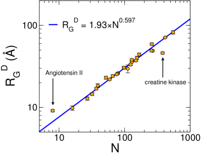
(a)

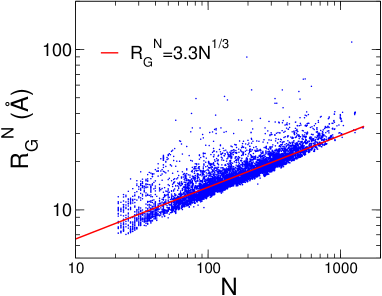
(b)

Figure 1:

(a)

$\begin{array}[]{cc}\begin{lx@subfloat@@figure}\includegraphics[width=173.44534pt]{Fig2B}\@@toccaption{{\lx@tag[ ]{{b}}{}}}\@@caption{{\lx@tag[ ]{{(b)}}{}}}\end{lx@subfloat@@figure}&\begin{lx@subfloat@@figure}\includegraphics[width=173.44534pt]{Fig2C}\@@toccaption{{\lx@tag[ ]{{c}}{}}}\@@caption{{\lx@tag[ ]{{(c)}}{}}}\end{lx@subfloat@@figure}\end{array}$

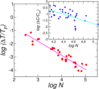
(b)

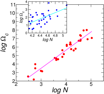
(c)

Figure 2:

$\begin{array}[]{cc}\begin{lx@subfloat@@figure}\includegraphics[width=216.81pt]{Fig3a}\@@toccaption{{\lx@tag[ ]{{a}}{}}}\@@caption{{\lx@tag[ ]{{(a)}}{}}}\end{lx@subfloat@@figure}&\begin{lx@subfloat@@figure}\includegraphics[width=312.20692pt]{Fig3b}\@@toccaption{{\lx@tag[ ]{{b}}{}}}\@@caption{{\lx@tag[ ]{{(b)}}{}}}\end{lx@subfloat@@figure}\\ \begin{lx@subfloat@@figure}\includegraphics[width=260.17464pt]{Fig3c}\@@toccaption{{\lx@tag[ ]{{c}}{}}}\@@caption{{\lx@tag[ ]{{(c)}}{}}}\end{lx@subfloat@@figure}&\begin{lx@subfloat@@figure}\includegraphics[width=173.44534pt]{Fig3d}\@@toccaption{{\lx@tag[ ]{{d}}{}}}\@@caption{{\lx@tag[ ]{{(d)}}{}}}\end{lx@subfloat@@figure}\end{array}$

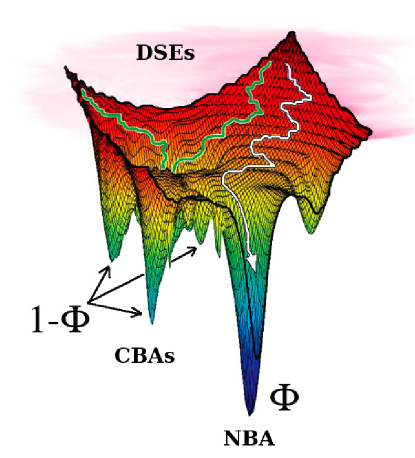
(a)

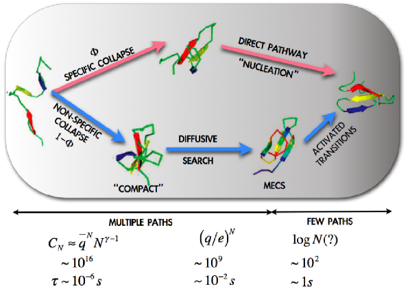
(b)

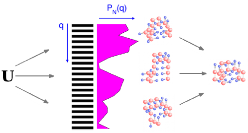
(c)

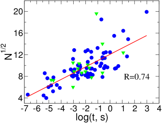
(d)

Figure 3:

$\begin{array}[]{cc}\begin{lx@subfloat@@figure}\includegraphics[width=173.44534pt]{Fig4a}\@@toccaption{{\lx@tag[ ]{{a}}{}}}\@@caption{{\lx@tag[ ]{{(a)}}{}}}\end{lx@subfloat@@figure}&\begin{lx@subfloat@@figure}\includegraphics[width=173.44534pt]{Fig4b}\@@toccaption{{\lx@tag[ ]{{b}}{}}}\@@caption{{\lx@tag[ ]{{(b)}}{}}}\end{lx@subfloat@@figure}\\ \qquad\qquad\begin{lx@subfloat@@figure}\includegraphics[width=173.44534pt]{Fig4c}\@@toccaption{{\lx@tag[ ]{{c}}{}}}\@@caption{{\lx@tag[ ]{{(c)}}{}}}\end{lx@subfloat@@figure}&\qquad\begin{lx@subfloat@@figure}\includegraphics[width=173.44534pt]{Fig4d}\@@toccaption{{\lx@tag[ ]{{d}}{}}}\@@caption{{\lx@tag[ ]{{(d)}}{}}}\end{lx@subfloat@@figure}\end{array}$

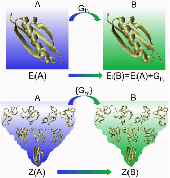
(a)

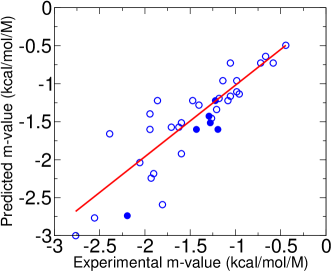
(b)

(c)

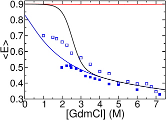
(d)

Figure 4:

$\begin{array}[]{ccc}\begin{lx@subfloat@@figure}\includegraphics[width=164.77771pt]{Fig5a}\@@toccaption{{\lx@tag[ ]{{a}}{}}}\@@caption{{\lx@tag[ ]{{(a)}}{}}}\end{lx@subfloat@@figure}&\begin{lx@subfloat@@figure}\includegraphics[width=182.1196pt]{Fig5b}\@@toccaption{{\lx@tag[ ]{{b}}{}}}\@@caption{{\lx@tag[ ]{{(b)}}{}}}\end{lx@subfloat@@figure}&\begin{lx@subfloat@@figure}\includegraphics[width=173.44534pt]{Fig5c}\@@toccaption{{\lx@tag[ ]{{c}}{}}}\@@caption{{\lx@tag[ ]{{(c)}}{}}}\end{lx@subfloat@@figure}\\ \qquad\qquad\begin{lx@subfloat@@figure}\includegraphics[width=151.76964pt]{Fig5d}\@@toccaption{{\lx@tag[ ]{{d}}{}}}\@@caption{{\lx@tag[ ]{{(d)}}{}}}\end{lx@subfloat@@figure}&\qquad\begin{lx@subfloat@@figure}\includegraphics[width=151.76964pt]{Fig5e}\@@toccaption{{\lx@tag[ ]{{e}}{}}}\@@caption{{\lx@tag[ ]{{(e)}}{}}}\end{lx@subfloat@@figure}&\begin{lx@subfloat@@figure}\includegraphics[width=173.44534pt]{Fig5f}\@@toccaption{{\lx@tag[ ]{{f}}{}}}\@@caption{{\lx@tag[ ]{{(f)}}{}}}\end{lx@subfloat@@figure}\end{array}$

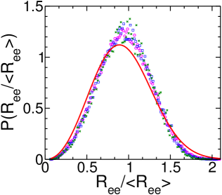
(a)

(b)

(c)

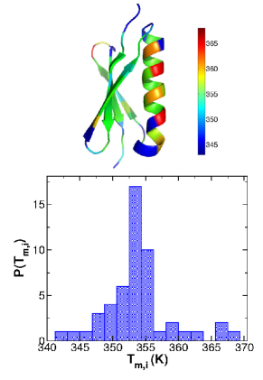
(d)

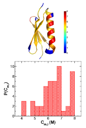
(e)

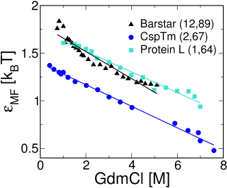
(f)

Figure 5:

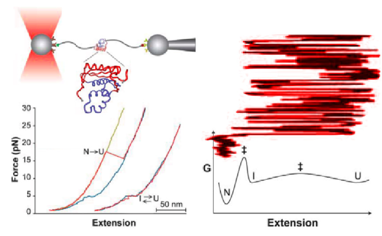
Figure 6:

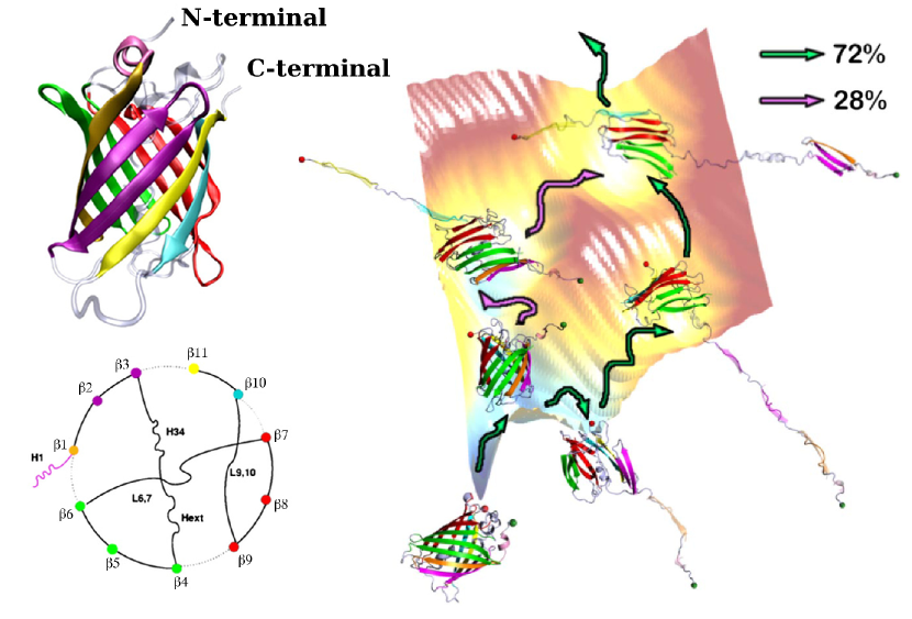
Figure 7:

$\begin{array}[]{c}\begin{lx@subfloat@@figure}\includegraphics[width=346.89731pt]{Fig8a}\@@toccaption{{\lx@tag[ ]{{a}}{}}}\@@caption{{\lx@tag[ ]{{(a)}}{}}}\end{lx@subfloat@@figure}\\ \begin{lx@subfloat@@figure}\includegraphics[width=346.89731pt]{Fig8b}\@@toccaption{{\lx@tag[ ]{{b}}{}}}\@@caption{{\lx@tag[ ]{{(b)}}{}}}\end{lx@subfloat@@figure}\end{array}$

(a)

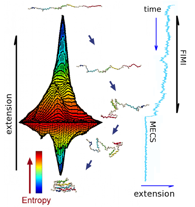
(b)

Figure 8:

$\begin{array}[]{c}\begin{lx@subfloat@@figure}\includegraphics[width=294.85841pt]{Fig9a}\@@toccaption{{\lx@tag[ ]{{a}}{}}}\@@caption{{\lx@tag[ ]{{(a)}}{}}}\end{lx@subfloat@@figure}\\ \begin{lx@subfloat@@figure}\includegraphics[width=346.89731pt]{Fig9b}\@@toccaption{{\lx@tag[ ]{{b}}{}}}\@@caption{{\lx@tag[ ]{{(b)}}{}}}\end{lx@subfloat@@figure}\end{array}$

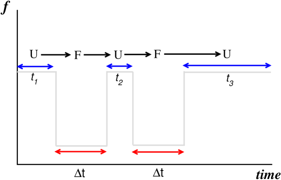
(a)

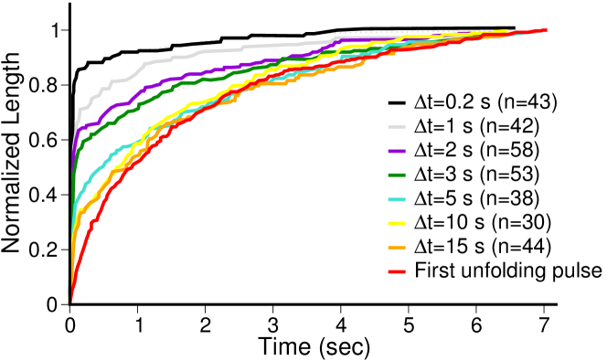
(b)

Figure 9:

References

- [1] Abkevich VI, Gutin AM, Shakhnovich EI 1994, Specific nucleus as the transition-state for protein-folding : Evidence from the lattice model. Biochemistry, 33:10026–10036.
- [2] Ainavarapu SRK, Brujic J, Huang HH, Wiita AP, Lu H, et al. 2007, Contour length and refolding rate of a small protein controlled by engineered disulfide bonds. Biophys. J., 92:225–233.
- [3] Anfinsen CB 1973, Principles that goven the folding of protein chain. Science, 181:223–230.
- [4] Auton M, Holthauzen LMF, Bolen DW 2007, Anatomy of energetic changes accompanying urea-induced protein denaturation. Proc. Natl. Acad. Sci., 104:15317–15322.
- [5] Baker D 2000, A surprising simplicity to protein folding. Nature, 405:39–42.
- [6] Baldwin RL, Rose GD 1999, Is protein folding hierarchic? II. Folding intermediates and transition states. TIBS, 24:77–83.
- [7] Barsegov V, Thirumalai D 2005, Probing protein-protein interactions by dynamic force correlation spectroscopy. Phys. Rev. Lett., 95:168302.
- [8] Bartlett AI, Radford SE 2009, An expanding arsenal of experimental methods yields an explosion of insights into protein folding mechanisms. Nat. Struct. & Mol. Biol., 16:582–588.
- [9] Block SM, Asbury CL, Shaevitz JW, Lang MJ 2003, Probing the kinesin reaction cycle with a 2D optical force clamp. Proc. Natl. Acad. Sci., 100:2351–2356.
- [10] Bolen DW, Rose GD 2008, Structure and energetics of the hydrogen-bonded backbone in protein folding. Annu. Rev. Biochem., 77:339–362.
- [11] Bradley P, Misura KMS, Baker D 2005, Toward high-resolution de novo structure prediction for small proteins. Science, 309:1868–1871.
- [12] Bryngelson JD, Wolynes PG 1989, Intermediates and barrier crossing in a random energy-model (with applications to protein folding). J. Phys. Chem., 93:6902–6915.
- [13] Bryngelson JD, Wolynes PG 1990, A Simple Statistical Field Theory of Heteropolymer Collapse with Application to Protein Folding. Biopolymers, 30:177–188.
- [14] Buscaglia M, Kubelka J, Eaton WA, Hofrichter J 2005, Determination of ultrafast protein folding rates from loop formation dynamics. J. Mol. Biol., 347:657–664.
- [15] Bustamante C, Marko JF, Siggia ED, Smith S 1994, Entropic elasticity of -phase DNA. Science, 265:1599–1600.
- [16] Camacho CJ, Thirumalai D 1993a, Kinetics and thermodynamics of folding in model proteins. Proc. Natl. Acad. Sci. USA, 90:6369–6372.
- [17] Camacho CJ, Thirumalai D 1993b, Minimum Energy Compact Structures of Random Sequences of Heteropolymers. Phys. Rev. Lett., 71:2505–2508.
- [18] Cecconi C, Shank EA, Bustamante C, Marqusee S 2005, Direct Observation of Three-State Folding of a Single Protein Molecule. Science, 309:2057–2060.
- [19] Chen J, Bryngelson J, Thirumalai D 2008, Estimations of the size of nucleation regions in globular proteins. J. Phys. Chem. B, 112:16115–16120.
- [20] Cheung MS, Klimov D, Thirumalai D 2005, Molecular crowding enhances native state stability and refolding rates of globular proteins. Proc. Natl. Acad. Sci., 102:4753–4758.
- [21] Chiti F, Dobson C 2006, Protein misfolding, functional amyloid, and human disease. Annu. Rev. Biochem., 75:333–366.
- [22] Clementi C, Nymeyer H, Onuchic JN 2000, Topological and energetic factors: what determines the structural details of the transition state ensemble and “en-route” intermediates for protein folding? an investigation for small globular protein. J. Mol. Biol., 298:937–953.
- [23] de Gennes PG 1979, Scaling Concepts in Polymer Physics (Cornell University Press, Ithaca and London).
- [24] Dietz H, Berkemeier F, Bertz M, Rief M 2006, Anisotropic deformation response of single protein molecules. Proc. Natl. Acad. Sci., 103:12724–12728.
- [25] Dietz H, Rief M 2004, Exploring the energy landscape of GFP by single-molecule mechanical experiments. Proc. Natl. Acad. Sci., 101:16192–16197.
- [26] Dill KA, Bromberg S, Yue KZ, Fiebig KM, Yee DP, et al. 1995, Principles of protein-folding - a perspective from simple exact models. Prot. Sci., 4:561–602.
- [27] Dill KA, Chan HS 1997, From Levinthal to Pathways to Funnels. Nature Struct. Biol., 4:10–19.
- [28] Dill KA, Ozkan SB, Shell MS, Weikl TR 2008, The protein folding problem. Annu. Rev. Biophys., 37:289–316.
- [29] Dima RI, Thirumalai D 2004, Asymmetry in the shapes of folded and denatured states of proteins. J. Phys. Chem. B, 108:6564–6570.
- [30] Dobson CM, Sali A, Karplus M 1998, Protein folding: A perspective from theory and experiment. Angewandte Chemie-International Edition, 37:868–893.
- [31] Doi M, Edwards SF 1988, The Theory of Polymer Dynamics (Clarendon Press, Oxford).
- [32] Dudko OK, Filippov AE, Klafter J, Urbakh M 2003, Beyond the conventional description of dynamic force spectroscopy of adhesion bonds. Proc. Natl. Acad. Sci., 100:11378–11381.
- [33] Dudko OK, Hummer G, Szabo A 2006, Intrinsic rates and activation free energies from single-molecule pulling experiments. Phys. Rev. Lett., 96:108101.
- [34] Dudko OK, Hummer G, Szabo A 2008, Theory, Analysis, and Interpretation of Single-Molecule Force Spectroscopy Experiments. Proc. Natl. Acad. Sci., 105:15755–15760.
- [35] Eaton WA, Muñoz V, Hagen SJ, Jas GS, Lapidus LJ, et al. 2000, Fast Kinetics and Mechanisms in Protein Folding. Ann. Rev. Biophys. Biomol. Struct., 29:327–359.
- [36] Eisenberg D, Nelson R, Sawaya MR, Balbirnie M, Sambashivan S, et al. 2006, The structural biology of protein aggregation diseases: Fundamental questions and some answers. Acc. Chem. Res., 39:568–575.
- [37] Fernandez JM, Li H 2004, Force-clamp spectroscopy monitors the folding trajectory of a single protein. Science, 303:1674–1678.
- [38] Fersht A 1998, Structure and Mechanism in Protein Science : A Guide to Enzyme Catalysis and Protein Folding (W. H. Freeman Company).
- [39] Fersht AR 1995, Optimization of rates of protein-folding: The nucleation-condensation mechanism and its implications. Proc. Natl. Acad. Sci., 92:10869–10873.
- [40] Finkelstein AV, Badretdinov AY 1997, Rate of protein folding near the point of thermodynamic equilibrium between the coil and the most stable chain fold. Folding and Design, 2:115–121.
- [41] Fisher TE, Oberhauser AF, Carrion-Vazquez M, Marszalek PE, Fernandez JM 1999, The study of protein mechanics with the atomic force microscope. TIBS, 24:379–384.
- [42] Flory PJ 1971, Principles of Polymer Chemistry (Cornell University Press, Ithaca).
- [43] Forman JR, Clarke J 2007, Mechanical unfolding of proteins: insights into biology, structure and folding. Curr. Opin. Struct. Biol., 17:58–66.
- [44] Gambinand Y, Schug A, Lemke EA, Lavinder JJ, Ferreon ACM, et al. 2009, Direct single-molecule observation of a protein living in two opposed native structures. Proc. Natl. Acad. Sci., 106:10153–10158.
- [45] Garcia-Manyesa S, Dougana L, Badillaa CL, Brujic J, Fernandez JM 2009, Direct observation of an ensemble of stable collapsed states in the mechanical folding of ubiquitin. Proc. Natl. Acad. Sci., 106:10534?10539.
- [46] Golouginoff P, Gatenby AA, Lorimer GH 1989, GroEL heat-shock proteins promote assembly of foreign prokaryotic ribulose bisphosphate carboxylase oligomers in Escherichia-Coli. Nature, 337:44–47.
- [47] Gosavi S, Chavez LL, Jennings PA, Onuchic JN 2006, Topological frustration and the folding of interleukin-1. J. Mol. Biol., 357:986–96.
- [48] Gosavi S, Whitford PC, Jennings PA, Onuchic JN 2008, Extracting function from a -trefoil folding motif. Proc. Natl. Acad. Sci., 105:10384–10389.
- [49] Grosberg AY, Khokhlov AR 1994, Statistical Physics of Macromolecules (AIP Press).
- [50] Guo Z, Thirumalai D 1995, Kinetics of Protein Folding: Nucleation Mechanism, Time Scales, and Pathways. Biopolymers, 36:83–102.
- [51] Gutin AM, Abkevich VI, Shakhnovich EI 1996, Chain Length Scaling of Protein Folding Time. Phys. Rev. Lett., 77:5433–5436.
- [52] Hammond GS 1953, A correlation of reaction rates. J. Am. Chem. Soc., 77:334–338.
- [53] Hanggi P, Talkner P, Borkovec M 1990, Reaction-rate theory: fifty years after Kramers. Rev. Mod. Phys., 62:251–341.
- [54] Haran G 2003, Single-molecule fluorescence spectroscopy of biomolecular folding. J. Phys. Cond. Matt., 15:R1291–R1317.
- [55] Hills RD, Brooks CL 2009, Insights from Coarse-Grained Go Models for Protein Folding and Dynamics. Itnl. J. Mol. Sci., 10:889–905.
- [56] Holtzer ME, Lovett EG, d Avignon DA, Holtzer A 1997, Thermal unfolding in a GCN4-like leucine zipper: C-13 R NMR chemical shifts and local unfolding. Biophys. J., 73:1031–1041.
- [57] Honeycutt JD, Thirumalai D 1990, Metastability of the folded state of globular proteins. Proc. Natl. Acad. Sci., 87:3526–3529.
- [58] Horwich AL, Farr GW, Fenton WA 2006, GroEL-GroES-mediated protein folding. Chem. Rev., 106:1917–1930.
- [59] Hyeon C, Dima RI, Thirumalai D 2006, Pathways and kinetic barriers in mechanical unfolding and refolding of RNA and proteins. Structure, 14:1633–1645.
- [60] Hyeon C, Morrison G, Pincus DL, Thirumalai D 2009, Refolding dynamics of stretched biopolymers upon force-quench. Proc. Natl. Acad. Sci.
- [61] Hyeon C, Morrison G, Thirumalai D 2008, Force dependent hopping rates of RNA hairpins can be estimated from accurate measurement of the folding landscapes. Proc. Natl. Acad. Sci., 105:9604–9606.
- [62] Hyeon C, Thirumalai D 2003, Can energy landscape roughness of proteins and RNA be measured by using mechanical unfolding experiments? Proc. Natl .Acad. Sci., 100:10249–10253.
- [63] Hyeon C, Thirumalai D 2007a, Measuring the energy landscape roughness and the transition state location of biomolecules using single molecule mechanical unfolding experiments. J. Phys.: Condens. Matter, 19:113101.
- [64] Hyeon C, Thirumalai D 2007b, Mechanical unfolding of RNA : from hairpins to structures with internal multiloops. Biophys. J., 92:731–743.
- [65] Itzhaki LS, Otzen DE, Fersht AR 1995, The structure of the transition-state for folding of chymotrypsin inhibitor-2 analyzed by protein engineering methods - evidence for a nucleation-condensation mechanism for protein-folding. J. Mol. Biol., 254:260–288.
- [66] Janovjak H, Knaus H, Muller DJ 2007, Transmembrane helices have rough energy surfaces. J. Am. Chem. Soc., 129:246–247.
- [67] Jha SK, Dhar D, Krishnamoorthy G, Udgaonkar JB 2009, Continuous dissolution of structure during the unfolding of a small protein. Proc. Natl. Acad. Sci., 106:11113–11118.
- [68] Karanicolas J, Brooks CL 2003, Improved Go-like models demonstrate the robustness of protein folding mechanisms towards non-native interactions. J. Mol. Biol., 334:309–325.
- [69] Karanicolas J, Brooks CL 2004, Integrating folding kinetics and protein function: Biphasic kinetics and dual binding specificity in a WW domain. Proc. Natl. Acad. Sci., 101:3432–3437.
- [70] Kendrew JC 1961, The three-dimensional structure of a protein molecule. Sci. Am., 205:96–110.
- [71] Kiefhaber T 1995, Kinetic traps in lysozyme folding. Proc. Natl. Acad. Sci., 92:9029–9033.
- [72] Kleiner H, Schulte-Flohlinde V 2002, Critical Properties of -Theories (World Scientific).
- [73] Klimov DK, Thirumalai D 1996, Factors governing the foldability of proteins. Prot. Struct. funct. Genetics, 26:411–441.
- [74] Klimov DK, Thirumalai D 1998a, Cooperativity in Protein Folding: From Lattice Models with Side Chanins to Real Proteins. Folding Des., 3:127–139.
- [75] Klimov DK, Thirumalai D 1998b, Linking rates of folding in lattice models of proteins with underlying thermodynamic characteristics. J. Chem. Phys., 109:4119–4125.
- [76] Klimov DK, Thirumalai D 1999, Stretching single-domain proteins: Phase diagram and kinetics of force-induced unfolding. Proc. Natl. Acad. Sci., 96:6166–6170.
- [77] Klimov DK, Thirumalai D 2001, Multiple protein folding nuclei and the transition state ensemble in two-state proteins. Proteins - Struct. Funct. Gene., 43:465–475.
- [78] Klimov DK, Thirumalai D 2002, Stiffness of the distal loop restricts the structural heterogeneity of the transition state ensemble in SH3 domains. J. Mol. Biol., 317:721–737.
- [79] Klimov DK, Thirumalai D 2005, Symmetric connectivity of secondary structure elements enhances the diversity of folding pathways. J. Mol. Biol., 353:1171–1186.
- [80] Kohn JE, Millett IS, Jacob J, Azgrovic B, Dillon TM, et al. 2004, Random-coil behavior and the dimensions of chemically unfolded proteins. Proc. Natl. Acad. Sci., 101:12491–?12496.
- [81] Kramers HA 1940, Brownian motion a field of force and the diffusion model of chemical reaction. Physica, 7:284–304.
- [82] Kubelka J, Hofrichter J, Eaton W 2004, The protein folding ‘speed limit’. Curr. Opin. Struct. Biol., 14:76–88.
- [83] Lakshmikanth GS, Sridevi K, Krishnamoorthy G, Udgaonkar JB 2001, Structure is lost incrementally during the unfolding of barstar. Nat. Struct. Biol., 8:799–804.
- [84] Leopold PE, Montal M, Onuchic JN 1992, Protein folding funnels: a kinetic approach to the sequence-structure relationship. Proc. Natl. Acad. Sci., 89:8721–8725.
- [85] Levitt M, Warshel A 1975, Computer-simulation of protein folding. Nature, 253:694–698.
- [86] Li H, Mirny L, Shakhnovich EI 2000, Kinetics, thermodynamics and evolution of non-native interactions in a protein folding nucleus. Nat. Struct. Biol., 7:336–342.
- [87] Li MS, Hu CK, Klimov DK, Thirumalai D 2006, Multiple stepwise refolding of immunoglobulin I27 upon force quench depends on initial conditions. Proc. Natl. Acad. Sci., 103:93–98.
- [88] Li MS, Klimov DK, Thirumalai D 2004, Finite size effects on thermal denaturation of globular proteins. Phys. Rev. Lett., 93:268107.
- [89] Liphardt J, Onoa B, Smith SB, Tinoco Jr. I, Bustamante C 2001, Reversible Unfolding of Single RNA Molecules by Mechanical Force. Science, 292:733–737.
- [90] Lipman EA, Schuler B, Bakajin P, Eaton WA 2003, Single-molecule measurement of protein folding kinetics. Science, 301:1233–1235.
- [91] Marko JF, Siggia ED 1995, Stretching DNA. Macromolecules, 28:8759–8770.
- [92] Matthews CR 1993, Pathways of protein-folding. Ann. Rev. Biochem., 62:653–683.
- [93] Merchant KA, Best RB, Louis JM, Gopich IV, Eaton W 2007, Characterizing the unfolded states of proteins using single-molecule FRET spectroscopy and molecular simulations. Proc. Natl. Acad. Sci. USA, 104:1528–1533.
- [94] Merkel R, Nassoy P, Leung A, Ritchie K, Evans E 1999, Energy landscapes of receptor-ligand bonds explored with dynamic force spectroscopy. Nature, 397:50–53.
- [95] Mézard M, Parisi G, Virasoro M 1988, Spin glass theory and beyond (World Scientific).
- [96] Mickler M, Dima RI, Dietz H, Hyeon C, Thirumalai D, Rief M 2007, Revealing the bifurcation in the unfolding pathways of GFP by using single-molecule experiments and simulations. Proc. Natl. Acad. Sci., 104:20268–20273.
- [97] Moult J 2005, A decade of CASP: progress, bottlenecks and prognosis in protein structure prediction. Curr. Opin. Struct. Biol., 15:285–289.
- [98] Naganathan AN, Sanchez-Ruiz JM, Muñoz V 2005, Direct measurement of barrier heights in protein folding. J. Am. Chem. Soc., 127:17970–17971.
- [99] Nevo R, Brumfeld V, Kapon R, Hinterdorfer P, Reich Z 2005, Direct measurement of protein energy landscape roughness. EMBO reports, 6:482.
- [100] Nienhaus GU 2006, Exploring protein structure and dynamics under denaturing conditions by single-molecule FRET analysis. Macro. Biosci., 6:907–922.
- [101] Nymeyer H, Socci N, Onuchic J 2000, Landscape approaches for determining the ensemble of folding transition states : Success and failure hinge on the degree of frustration. Proc. Natl. Acad. Sci. USA, 97:634–639.
- [102] O’Brien EP, Brooks BR, Thirumalai D 2009, Molecular origin of constant m-values, denatured state collapse, and residue-dependent transition midpoints in globular proteins. Biochemistry, 48:3743–3754.
- [103] O’Brien EP, Ziv G, Haran G, Brooks BR, Thirumalai D 2008, Denaturant and osmolyte effects on proteins are accurately predicted using the Molecular Transfer Model. Proc. Natl. Acad. Sci. USA, 105:13403–13408.
- [104] Onoa B, Dumont S, Liphardt J, Smith SB, Tinoco, Jr. I, Bustamante C 2003, Identifying Kinetic Barriers to Mechanical Unfolding of the T. thermophila Ribozyme. Science, 299:1892–1895.
- [105] Onuchic J, Luthey-Schulten Z, Wolynes PG 1997, Theory of Protein Folding: The Energy Landscape Perspective. Ann. Rev. Phys. Chem., 48:539–600.
- [106] Onuchic JN, Wolynes PG 2004, Theory of protein folding. Curr. Opin. Struct. Biol., 14:70–75.
- [107] Peng Q, Li H 2008, Atomic force microscopy reveals parallel mechanical unfolding pathways of T4 lysozyme: Evidence for a kinetic partitioning mechanism. Proc. Natl. Acad. Sci., 105:1885–1890.
- [108] Ramakrishnan TV, Yussoff M 1979, First-principles order-parameter theory of freezing. Phys. Rev. B., 19:2775–2794.
- [109] Rhoades E, Cohen M, Schuler B, Haran G 2004, Two-state folding observed in individual protein molecules. J. Am. Chem. Soc., 126:14686–14687.
- [110] Rhoades E, Gussakovsky E, Haran G 2003, Watching proteins fold one molecule at a time. Proc. Natl. Acad. Sci., 100:3197–3202.
- [111] Roder H, Col?n W 1997, Kinetic role of early intermediates in protein folding. Curr. Opin. Struct. Biol., 7:15–28.
- [112] Sadqi M, Fushman D, Muñoz V 2006, Atom-by-atom analysis of global downhill protein folding. Nature, 442:317–321.
- [113] Schlierf M, Rief M 2005, Temperature softening of a protein in single-molecule experiments. J. Mol. Biol., 354:497–503.
- [114] Schuler B, Eaton WA 2008, Protein folding studied by single-molecule FRET. Curr. Opin. Struct. Biol., 18:16–26.
- [115] Schuler B, Lipman EA, Eaton WA 2002, Probing the free-energy surface for protein folding with single-molecule fluorescence spectroscopy. Nature, 419:743–747.
- [116] Selkoe DJ 2003, Folding proteins in fatal ways. Nature, 426:900–904.
- [117] Shakhnovich E 2006, Protein folding thermodynamics and dynamics: Where physics, chemistry, and biology meet. Chem. Rev., 106:1559–1588.
- [118] Shea JE, Brooks CL 2001, From folding theories to folding proteins: A review and assessment of simulation studies of protein folding and unfolding. Ann. Rev. Phys. Chem., 52:499–535.
- [119] Sherman E, Haran G 2006, Coil-globule transition in the denatured state of a small protein. Proc. Natl. Acad. Sci., 103:11539–11543.
- [120] Snow CD, Sorin EJ, Rhee YM, Pande VS 2005, How well can simulation predict protein folding kinetics and thermodynamics? Ann. Rev. Biophys. Biomol. Struct., 34:43–69.
- [121] Spagnolo L, Ventura S, Serrano L 2003, Folding specificity induced by loop stiffness. Protein Sci., 12:1473–1482.
- [122] Tehver R, Thirumalai D 2008, Kinetic model for the coupling between allosteric transitions in groel and substrate protein folding and aggregation. J. Mol. Biol., 4:1279–1295.
- [123] Thirumalai D 1995, From Minimal Models to Real Proteins: Time Scales for Protein Folding Kinetics. J. Phys. I (Fr.), 5:1457–1467.
- [124] Thirumalai D, Guo ZY 1995, Nucleation mechanism for protein-folding and theoretical predictions for hydrogen-exchange labeling experiments. Biopolymers, 35:137–140.
- [125] Thirumalai D, Hyeon C 2005, RNA and Protein folding: Common Themes and Variations. Biochemistry, 44:4957–4970.
- [126] Thirumalai D, Klimov D, Dima R 2003, Emerging ideas on the molecular basis of protein and peptide aggregation. Curr. Opin. Struct. Biol., 13:146–159.
- [127] Thirumalai D, Klimov DK 1999, Deciphering the Time Scales and Mechanisms of Protein Folding Using Minimal Off-Lattice Models. Curr. Opin. Struct. Biol., 9:197–207.
- [128] Thirumalai D, Lorimer GH 2001, Chaperonin-mediated protein folding. Ann. Rev. Biophys. Biomol. Struct., 30:245–269.
- [129] Thirumalai D, Mountain R, Kirkpatrick T 1989, Ergodic behavior in supercooled liquids and in glasses. Phys. Rev. A., 39:3563–3574.
- [130] Thirumalai D, Woodson SA 1996, Kinetics of Folding of Proteins and RNA. Acc. Chem. Res., 29:433–439.
- [131] Tinoco Jr. I 2004, Force as a useful variable in reactions: Unfolding RNA. Ann. Rev. Biophys. Biomol. Struct., 33:363–385.
- [132] Todd MJ, Lorimer GH, Thirumalai D 1996, Chaperonin-facilitated protein folding: Optimization of rate and yield by an iterative annealing mechanism. Proc. Natl. Acad. Sci., 93:4030–4035.
- [133] Udgaonkar JB 2008, Multiple routes and structural heterogeneity in protein folding. Ann. Rev. Biophys., 37:489–510.
- [134] Visscher K, Schnitzer MJ, Block SM 1999, Single kinesin molecules studied with a molecular force clamp. Nature, 400:184–187.
- [135] Wolynes PG 1996, Symmetry and the energy landscapes of biomolecules. Proc. Natl. Acad. Sci., 93:14249–14255.
- [136] Wolynes PG 1997, Folding funnels and energy landscapes of larger proteins within the capillarity approximation. Proc. Natl. Acad. Sci., 94:6170–6175.
- [137] Woodside MT, Anthony PC, Behnke-Parks WM, Larizadeh K, Herschlag D, Block SM 2006a, Direct measurement of the full, sequence-dependent folding landscape of a nucleic acid. Science, 314:1001–1004.
- [138] Woodside MT, Behnke-Parks WM, Larizadeh K, Travers K, Herschlag D, Block SM 2006b, Nanomechanical measurements of the sequence-dependent folding landscapes of single nucleic acid hairpins. Proc. Natl. Acad. Sci., 103:6190–6195.
- [139] Woodside MT, Garcia-Garcia C, Block SM 2008, Folding and unfolding single RNA molecules under tension. Curr. Opin. Chem. Biol., 12:640–646.
- [140] Xu Z, Horwich AL, Sigler PB 1997, The crystal structure of the asymmetric GroEL-GroES-(ADP)7 chaperonin complex. Nature, 388:741.
- [141] Yang WY, Gruebele M 2003, Folding at the speed limit. Nature, 423:193 – 197.
- [142] Zhou HX, Rivas G, Minton AP 2008, Macromolecular crowding and confinement: Biochemical, biophysical, and potential physiological consequences. Ann. Rev. Biophys., 37:375–397.
- [143] Ziv G, Haran G 2009, Protein Folding, Protein Collapse, and Tanford’s Transfer Model: Lessons from Single-Molecule FRET. J. Am. Chem. Soc., 131:2942–2947.
- [144] Ziv G, Thirumalai D, Haran G 2009, Collapse transition in proteins. Phys. Chem. Chem. Phys., 11:83–93.