Studying of decays within supersymmetry
Abstract
Recent results from CDF Collaboration favor a large CP asymmetry in decay, while the Standard Model prediction is very small. Moreover, the measurement of its branching ratio is lower than the Standard Model prediction based on the QCD factorization. We compute the gluino-mediated supersymmetry contributions to , decays in the frame of the mass insertion method, and find that for , the theoretical predictions including the LR and RL mass insertion contributions are compatible with the measurements of decay and mixing within ranges. Using the constrained LR and RL mass insertion parameter spaces, we explore the supersymmetry mass insertion effects on the branching ratios, the direct CP asymmetries and the polarization fractions in decays. We find the constrained LR and RL insertions can provide sizable contributions to the branching ratios of , as well as the direct CP asymmetry and the longitudinal polarization of decay without conflict with all related data within ranges. Near future experiments at Fermi Lab and CERN LHC-b can test our predictions and shrink/reveal the mass insertion parameter spaces.
PACS Numbers: 12.60.Jv, 12.15.Ji, 12.38.Bx, 13.25.Hw
1 Introduction
In the recent ten years, the successful running of factories BABAR and Belle has provided rich experimental data for and , which has confirmed the Kobayashi-Maskawa CP asymmetry mechanism in the Standard Model (SM) and also shown hints for new physics (NP). Among the rich phenomena of decays, the decay modes of mesons into pairs of charmless mesons are the known effective probes of the CP violation in the SM and are sensitive to potential NP scenarios beyond the SM. The two body charmless decays will play the similar role in studying the CP asymmetries (CPA), determining CKM matrix elements and constraining/searching for the indirect effects of various NP scenarios. Recently the CDF Collaboration at Fermilab Tevatron has made the first measurement of charmless two-body decay [1, 2, 3, 4]
| (1) |
The measurement is important for understanding physics, and also implies that many decay modes could be precisely measured at the LHC-b.
Compared with the theoretical predictions for these quantities in Refs. [6, 7, 5], based on the QCD factorization (QCDF) [8], the perturbative QCD (PQCD) [9], and the soft-collinear effective theory (SCET) [10], respectively, one would find the experimental measurement of this branching ratio agrees with the SM predictions with SCET [5], but lower than the predictions with QCDF and PQCD [6, 7]. For the CDF measurement of , its central value favors a large CP violation in decay (different from 0 at ), although it is also compatible with zero. In Refs. [11, 12], a robust test of the SM or a probe of NP is suggested by comparison of the direct CP asymmetry in decay.
The decays , have been extensively studied in the literatures (for example, Refs. [6, 13, 7, 11, 12, 5, 14, 15, 16, 17]). The tree-dominated decays , are induced by transition at the quark level, where the direct CPA are expected to be small in the SM. At present, among many measurements in the similar modes of decays, several discrepancies with the SM predictions have appeared in tree-dominated processes, for example, puzzles [18, 19, 20, 21, 22]. Although the discrepancies are not statistically significant, there is an unifying similarity pointing to NP (for example, Refs. [23, 24, 25]). There could be also potential NP contributions in , decays. The measurement given in Eq. (1) will afford an opportunity to search/constrain NP scenarios beyond the SM.
Supersymmetry (SUSY) is an extension of the SM which emerges as one of the most promising candidates for NP beyond the SM. In SUSY, supersymmetric version of the SM contributes to the Flavor Change Natural Current (FCNC) processes. The flavor-changing in these processes is intrinsically tied to usual CKM-induced flavor-changing of the SM (If that were the only new source of flavor physics, we would say the model is minimally flavor violating). But general SUSY is not minimally flavor violation. For general SUSY, a new source of flavor violation is introduced by the squark mass matrices, which usually can not be diagonalized on the same basis as the quark mass matrices. This means gluinos (and other gaugios) will have flavor-changing couplings to quarks and squarks, which implies the FCNCs are mediated by gluinos and thus have strong interaction strength. In order to analyze the phenomenology of non-minimally flavor violating interactions in general SUSY framework, it is helpful to rotate the effects so that they occur in squark propagators rather than in couplings, and to parameterize them in terms of dimensionless mass insertion (MI) parameters with and . In this paper, we work in the usual MI approximation [26, 27], and consider , decays, in general SUSY models, where flavor violation due to the gluino mediation can be important. The chargino-stop and the charged Higgs-top loop contributions are parametrically suppressed relative to the gluino contributions, and thus are ignored following [28, 29, 30, 27]. In our work, we also discuss the implications of mixing since the relevant MI parameters, that affect , decays, enter also in mixing. We consider the LR, RL, LL and RR four kinds of the MIs. We find that for , our predictions including the LR or RL MI effects are compatible with the measurements of decay and mixing within ranges, and the constrained both LR and RL MIs could significantly affect the polarization fractions of decay. While the constrained LL and RR insertions from mixing can not explain the possible large CP asymmetry and the small branching ratio of because of lacking the gluino mass enhancement in the decay. Therefore, with the ongoing -physics at Tevatron, in particular with the onset of the LHC-b experiment, we expect a wealth of decay data and measurements of these observables could restrict or reveal the parameter spaces of the LR and RL insertions in the near future.
The paper is arranged as follows. In Sec. 2, the relevant formulas for , decays and mixing are presented. We also tabulate the theoretical inputs in this section. Sec. 3 deals with the numerical results. Using our constrained MI parameter spaces from decay and mixing, we explore the MI effects on the other observable quantities, which have not been measured yet in decays. Sec. 4 contains our summary and conclusion.
2 The theoretical frame
2.1 The decay amplitudes for , decays
2.1.1 The decay amplitudes in the SM
In the SM, the low energy effective Hamiltonian for the transition at the scale is given by [31]
| (2) |
here with are CKM factors, the Wilson coefficients within the SM can be found in Ref. [31], and the relevant operators are given as
| (3) |
where and are color indices, and .
With the weak effective Hamiltonian given in Eq. (2), one can write the decay amplitudes for the relevant two-body hadronic decays as
| (4) | |||||
The essential theoretical difficulty for obtaining the decay amplitude arises from the evaluation of hadronic matrix elements , for which we will employ the QCDF [8] throughout this paper. We will use the QCDF amplitudes of these decays derived in the comprehensive papers [6, 13] as inputs for the SM amplitudes.
2.1.2 SUSY effects in the decays
In SUSY extension of the SM with conserved R-parity, the potentially most important contributions to Wilson coefficients of penguins in the effective Hamiltonian arise from strong-interaction penguin and box diagrams with gluino-squark loops. They can contribute to the FCNC processes because the gluinos have flavor-changing coupling to the quark and squark eigenstates. In general SUSY, we only consider these potentially large gluino box and penguin contributions and neglect a multitude of other diagrams, which are parametrically suppressed by small electroweak gauge coupling [28, 29, 30, 27]. The relevant Wilson coefficients of process due to the gluino box or penguin diagram involving the LL and LR insertions are given (at the scale ) by [27, 32, 33, 34]
| (5) | |||||
where , and the loop functions can be found in Ref. [32]. For the RR and RL insertions, we have additional operators that are obtained by in the SM operators given in Eq. (3). The associated Wilson coefficients are either dominated by their expressions as above with the replacement . The remaining coefficients are either dominated by their SM or are electroweak penguins and therefore small.
The SUSY Wilson coefficients at low energy can be obtained from in Eq. (5) by using the renormalization group equation as discussed in Ref. [31]
| (6) |
where is the column vector of the Wilson coefficients and is the five-flavor evolution matrix. The detailed explicitness of is given in Ref. [31]. The coefficients and at the scale are given by [35, 36]
| (7) |
where .
2.1.3 The total decay amplitudes
For the LL and LR insertion, the NP effective operators have the same chirality with ones of the SM, so the total decays amplitudes can be obtained from the SM ones in Refs. [6, 13] by replacing
| (8) |
For RL and RR insertion, the NP effective operators have the opposite chirality with the SM ones, and we can get the corresponding decay amplitudes from the SM decay amplitudes by following replacements [37]
| (9) |
for and , as well as
| (10) |
for and .
Then the total branching ratios read
| (11) |
where is the lifetime, is the center of mass momentum in the center of mass frame of meson.
The direct CP asymmetry is defined as
| (12) |
In the decay, the two vector mesons have the same helicity, therefore three different polarization states are possible, one longitudinal and two transverse, and we define the corresponding amplitudes as . Transverse and helicity amplitudes are related by . Then we have
| (13) |
The longitudinal(transverse) polarization fraction () are defined by
| (14) |
2.2 Effective Hamiltonian for mixing
The most general mixing is described by the effective Hamiltonian [38]
| (15) |
with
| (16) |
where and the operators are obtained from by the exchange . The hadronic matrix elements, taking into account for renormalization effects, are defined as
| (17) |
with .
The Wilson coefficients receive contributions from both the SM and the SUSY loops: . In the SM, the box diagram generates only contribution to the operator , and the corresponding Wilson coefficient at the scale is [31]
| (18) |
where and is the QCD correction.
The gluino-mediated SUSY contributions to mixing and in the MI approximation have been extensively studied (for example, Refs. [42, 38, 40, 41]). In general SUSY models, there are new contributions to mixing from the gluino-squark box diagrams, and the corresponding Wilson coefficients (at the scale) are given by [28, 29, 30, 27]
| (19) |
The loop functions can be found in Ref. [32]. The other Wilson coefficients are obtained from by exchange of .
The SUSY Wilson coefficients at the scale can be obtained by
| (20) |
where . The magic number and can be found in Ref. [38]. Renormalization group evolution of is done in the same way as for .
2.3 Input Parameters
The input parameters are collected in Table 1. We have several remarks on the input parameters:
-
•
Wilson coefficients: The SM Wilson coefficients are obtained from the expressions in Ref. [31].
-
•
CKM matrix element: For the SM predictions, we use the CKM matrix elements from the Wolfenstein parameters of the latest analysis within the SM in Ref. [44], and for the SUSY predictions, we take the CKM matrix elements in terms of the Wolfenstein parameters of the NP generalized analysis results in Ref. [44].
-
•
Masses of SUSY particles: When we study the SUSY effects, we will consider each possible MI for only one at a time, neglecting the interferences between different insertions products, but keeping their interferences with the SM amplitude. We fix the common squark masses GeV and consider three values of (i.e. GeV) in all case.
3 Numerical results and analysis
Now we are ready to present our numerical results and analysis. First, we will show our estimations in the SM with the parameters listed in Table 1 and compare with the relevant experimental data. Then we will study the SUSY predictions for the branching ratios, the CP asymmetries and the polarization fractions in , decays. For CPA of , we will only study the longitudinal direct CP asymmetry ().
In the SM, the numerical results with error ranges for the sensitive parameters are presented in Table 2. The detailed error estimates corresponding to the different types of theoretical uncertainties have been already studied in Refs. [6, 13], and our SM results of , and are consistent with the ones in Refs. [6, 13].
| Decay modes | ( ) | ||
|---|---|---|---|
For the color-allowed tree-dominated decays ,,,, power corrections have limited impact, and the main sources of theoretical uncertainties in the branching ratios are the CKM matrix elements and the form factors. Their and can be predicted quite precisely, and found to be very small () due to small penguin amplitudes. The uncertainty of is mostly due to the uncertainties of different form factors. Comparing the SM predictions in Table 2 with the relevant experimental data in Eq. (1), we may see the present experimental data of the decay within ranges are not consistent with the SM predictions within error ranges of the input parameters. The experimental data of are obviously larger than the SM prediction, moreover, the measurement of its branching ratio is lower than the SM prediction based on the QCDF.
Now we turn to the gluino-mediated SUSY contributions to , decays in the framework of the MI approximation. These decays are induced by transition at the quark level, and we consider four kinds of MIs (LL, LR, RL and RR) contributing to , decays. In the SM, the very small direct CPA of these decays come from the weak phase of small penguin amplitudes. In order to have nonzero CPA, we need at least two independent amplitudes with different weak phases. In general SUSY models, we are considering, the weak phases reside in the complex MI parameters s and appear in the SUSY Wilson coefficients in Eq. (5). These weak phases are odd under a CP transformation.
First, we study constraints on the MI parameters , , and from decay and mixing. Using the formulas in Sec. 2.1 and the input parameters in Sec. 2.3, we may obtain the two-body branching ratios and the direct CPA of , decays within the framework of SUSY by the QCDF. The mass difference and CP phase of mixing are gotten from the formulas in Sec. 2.2 and the input parameters in Sec. 2.3. Noted that we take the relevant CKM matrix elements in terms of the Wolfenstein parameters of the NP generalized analysis results in [44], which is different from the SM predictions. In each of the MI scenarios to be discussed, we vary the mass insertions over the range to fully map the parameter space. We then impose experimental constraints from decay and mixing, which are shown in Eq. (1) and Eq. (22), respectively.
For the LL and RR MIs, and are strongly constrained from mixing [38, 40, 34, 41]. The effects of the constrained LL and RR insertions on are almost negligible because of lacking the gluino mass enhancement in the decay, and they will not provide any significant effect on and . The current data within (or ) ranges of cannot be explained by the LL and RR MIs.
The case of the LR or RL insertion is very different from that of either LL or RR insertion. The LR and RL MIs only generate (chromo)magnetic operators and , respectively. Especially, the LR and RL insertions are more strongly constrained, since their contributions are enhanced by due to the chirality flip from the gluino in the loop compared with the contribution including the SM one. In these cases, even a small or can have large effects in the decays.
We can not get the allowed spaces of the LR and RL insertion parameters which may explain all these data within ranges given in Eq. (1) and Eq. (22) at the same time. In fact, there is no common allowed parameter space from and within ranges. Using the central values of the input parameters and GeV, we show the contour plots of and in the and planes in Fig. 1.
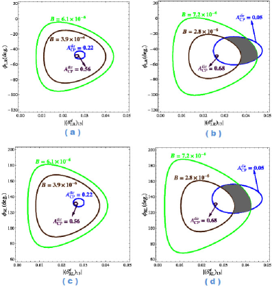
We discuss Fig. 1 (a) in detail. Fig. 1 (a) show the contour plot of error bars of and in plane. The space between the contour lines of and is the allowed space for within ranges. The space between the contour lines of and is the allowed space for within ranges. From Fig. 1 (a), we can see that there is no intersection between the allowed space from and the allowed space from , and the experimental data of within give quite strong constraints on . The similar results for the RL insertion are shown in Fig. 1 (c) in plane, and there is also no intersection between the allowed space from within ranges and the allowed space from within ranges.
Then we expand the experimental bounds within ranges to search for the allowed spaces of the LR and RL MI parameters. As shown in the dark gray ranges of Fig. 1 (b) and (d), there are the allowed spaces for the LR and RL insertion parameters from the data of decay within ranges. Noted that the allowed parameter spaces shown in the dark gray ranges of Fig. 1 (b) and (d) are obtained by using the central values of the input parameters. The allowed spaces will be enlarged if we consider the theoretical uncertainties of the input parameters. We use the experimental bounds of decay and mixing within ranges, and take the input parameters within ranges to obtain the allowed spaces of the LR and RL insertion parameters. The constrained spaces of and for GeV and different are demonstrated in Fig. 2, and the corresponding numerical ranges are summarized in Table 3.

| (deg.) | (deg.) | |||
|---|---|---|---|---|
In Fig. 2, we can see the allowed moduli of the LR and RL MI parameters are very sensitive to the values of , nevertheless the allowed phase ranges of the LR and RL MI parameters are not changed obviously for different . We find that both moduli and phases of are strongly constrained by the data of the decay within ranges, since the SM prediction of with the QCDF is not consistent with the experimental data within ranges. The lower limits of come from the experimental lower limit of within ranges. In the case of , are also constrained by within ranges, while sin within ranges doesn’t provide any further constraint. It’s different in the case of , are also constrained by sin within ranges, but within ranges doesn’t provide any further constraint.
It is worth to note that we also study the constrained spaces of and in the case of , and we find there is no intersection of the constrained spaces between from mixing within ranges and from decay within ranges. From mixing within ranges, we get , in which if , and if . We obtain from decay within ranges, in which () if , and () if . So there is no common allowed phases between the bounds from mixing and the bounds from decay in the case of . If , there still are common allowed spaces for the LR and RL MIs. For the LR MI, two very narrow allowed spaces are near and . For the RL MI, two very allowed spaces are near and .
The relevant upper bounds have been obtained in Refs. [38, 40, 41]. In Ref. [38], for , respectively, which are constrained by imposing the experimental bounds from and within ranges, setting GeV and scanning over the CKM phase . In Ref. [40], for GeV from and within ranges. In Ref. [41], for GeV from and . In the case of and , comparing with the exist bounds in [38, 40, 41], our upper limits of are at the same order of previous ones, while the lower limits of are also given from decay within ranges. In addition, are strongly constrained from decay. The allowed space for case are ruled out by both decay and mixing together.
Next, we will explore the SUSY effects on the other quantities, which have not been measured yet in , decays, by using the constrained parameter spaces of the LR and LR insertions as shown in Fig. 2. With the expressions for , and , we perform a scan through the input parameters within ranges and the new constrained SUSY MI parameter spaces, and then the allowed ranges for , and are obtained with different SUSY mixing insertion parameter, which satisfy relevant experimental constraints of decay given in Eq. (1) and mixing given in Eq. (22). The numerical results for with different value are summarized in Table 4.
| SUSY values | SUSY values | SUSY values | SUSY values | ||
| Observables | SM predictions | with | with | with | with |
| for | for | for | for | ||
The corresponding SM predictions with error ranges of the input parameters are also listed for comparison in the second column of the Table 4. We can see the data of is consistent with the SM prediction of at C.L., nonetheless very close the lower limit of its SM prediction. The data of is not consistent with its SM prediction at C.L.. From the last four columns of the Table 4, we can see the results are similar for different value of . In the SUSY predictions of the branching ratios, there are many sources of uncertainties, mainly arising from different form factors, CKM matrix elements, the annihilation contribution, other hadronic parameters of the QCDF, and the constrained MI parameters. The uncertainties of these direct CPA mostly come from the constrained MI parameters. The uncertainty of due to different form factors and the constrained MI parameters.
Comparing the SUSY predictions to the SM predictions given in Table 4, we give some remarks on the numerical results:
-
•
The LR and RL MIs have significant effects on , and the relevant parameters have been limited by both upper and lower limits of within ranges. The LR and RL MIs also have great effects on , which could be increased from the SM prediction range to about , however, the range is still far from the central value of its measurement, and is near to the lower limit of the measurement within ranges. The LR and RL MI parameters just have been limited by the lower limit of within ranges.
-
•
The constrained LR insertion still has significant effects on . The allowed lower limits of could be reduced one or two order(s) from their SM predictions, and the allowed upper limit of has been suppressed a lot from its SM prediction. In the SM, the direct CPA are very small in these decays. It is interesting to find the contributions of the constrained LR insertion have great effects on . The allowed ranges of could be extremely enlarged from ones of their tiny SM predictions. We find the constrained LR insertion contributions have a great impact on the longitudinal polarization fraction , which could be reduced to about zero by the constrained LR insertion.
-
•
For the RL MI case, the effects of the constrained RL insertion could exceedingly increase the allowed upper limits of and decrease the upper limit of . The RL insertion has small effects on , however, this insertion can greatly affect . also could be reduced to about zero by the constrained RL insertion.
Noted that the LR and RL MIs only generate dipole operators and , respectively, and , do not contribute to the transverse penguin amplitudes at due to angular momentum conservation in decay [51]. In other words, the LR and RL MIs only contribute to the longitudinal penguin amplitude at . Because the LR and RL contributions are enhanced by , even a small or can have large effects on the longitudinal penguin amplitude, and then can significantly affect the polarization fractions of decay. For the similar reason, the LR and RL MIs have been proposed as a possible resolution to the polarization puzzle in decays [52, 53].
For each LR and RL insertions, we can present the distributions and correlations of , , within the modulus or weak phase of the constrained MI parameter space in Fig. 2 by two-dimensional scatter plots.
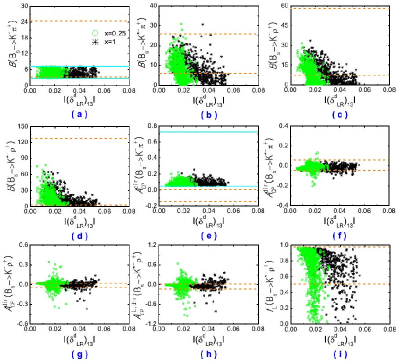
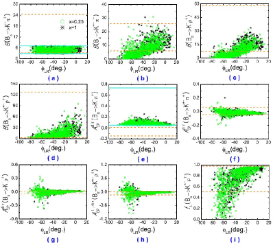
The LR MI effects on all observables of are displayed in Fig. 4 and Fig. 4. Fig. 4 shows the sensitivities of all observables to for different value of , and we see that all observables expect are a little sensitive to both and the values of . Fig. 4 displays the sensitivities of the observables to for different , and we can see that the weak phase for different value has similar allowed ranges, and has similar effects on every observable. In addition, for comparing conveniently, we show the SM bounds of these observables by orange horizontal dash lines and the limits of the measurements of within error-bar by the cyan horizontal solid lines. From Fig. 4(a-d) and Fig. 4(a-d), we see that is strongly constrained from its experimental data, are very sensitive to both and , and they are decreasing with but increasing with . As shown in Fig. 4(e) and Fig. 4(e), the LR insertion has positive effects on , and there is no any point in the SM area since is strongly constrained by the corresponding experimental data, which are not consistent with the SM predictions at 95% C.L.. Fig. 4 (f-h) and Fig. 4 (f-h) display that are sensitive to , and could have very large allowed ranges when . As for the LR insertion effects on , we show it in Fig. 4 (i) and Fig. 4 (i), and we can see could be hugely affected by the LR MI. has some sensitivities to both and , and it has smaller allowed range with . So the future measurement of could give obvious constraint on .
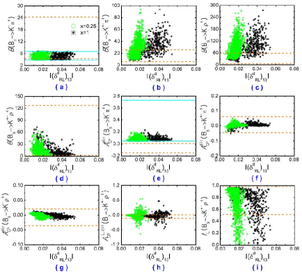

Next, we discuss the RL MI effects on all observables in decays. Fig. 6 and Fig. 6 show the observables as functions of and , respectively. Fig. 6(a,d) and Fig. 6(a,d) show the constrained RL MI has negative effects on , which is same as the LR MI effects on them. Fig. 6(b,c) and Fig. 6(b,c) show us the constrained RL MI has very large positive effects on , which is different from the LR MI. have some sensitivities to and as displayed in Fig. 6(b-d) and Fig. 6 (b-d). As shown in Fig. 6(f,g) and Fig. 6 (f,g), the RL MI has small effects on , and the RL insertion contributions can not be distinguished from the SM prediction. Fig. 6 (h) and Fig. 6 (h) show the RL MI effects on are similar to the LR insertion effects on it. could has very large allowed ranges when . As shown in Fig. 6 (i), could be strongly suppressed by the RL insertion, too.
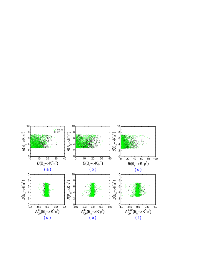
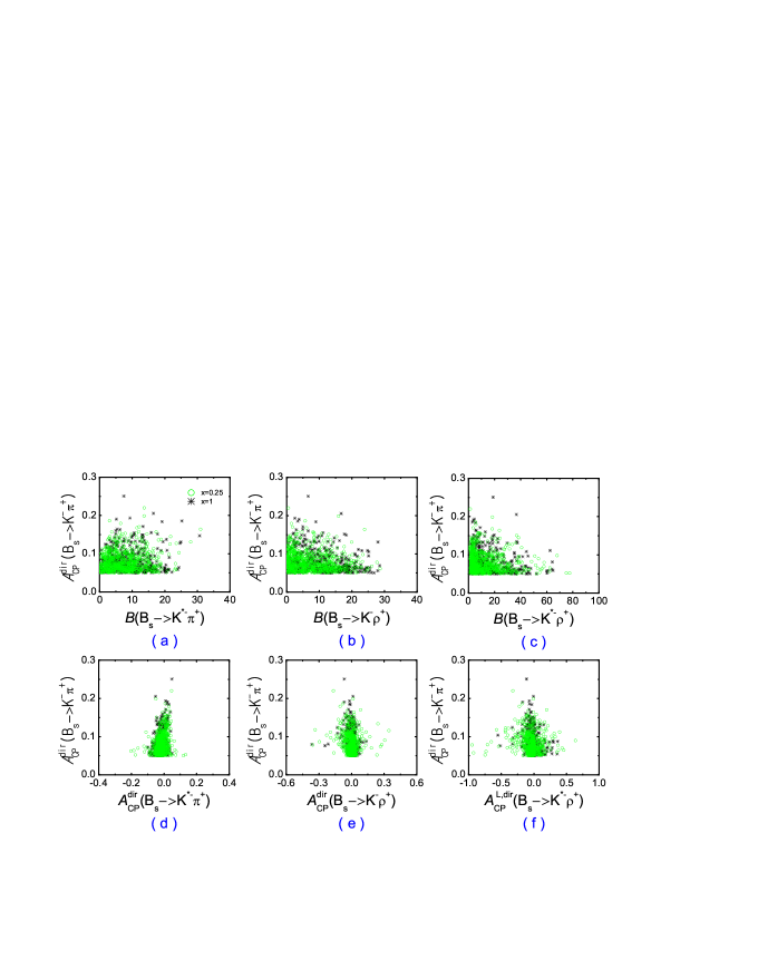
In addition, for the LR MI case, we show the resulting predictions for vs. and vs. in Fig. 8, as well as vs. and vs. in Fig. 8. In all plots in Fig. 8 and Fig. 8, the black and green points satisfy the constraints of decay and mixing within ranges. As displayed in Fig. 8, both and are not very sensitive to the constrained . However, as shown in Fig. 8, both and have some sensitivities to the constrained . Fig. 8 (a-c) show us, could has maximum when is near the lower limits of the SM predictions, and could have smaller allowed range with . Fig. 8 (d-f) indicate that there are some pionts accounting for large values of when is small.
There are similar correlations in the case of the RL MI as ones in Fig. 8 and Fig. 8 expect the correlations between and as well as between and . have no any sensitivities to and .
4 Conclusions
Motivated by recent results from CDF, which favor a possible large CP asymmetry and a small branching ratio in decay, we have studied the gluino-mediated SUSY contributions with the MIs to four decays based on the QCDF approach. For the LL and RR MIs, we have found that the constrained LL and RR insertion effects from mixing are almost negligible in decays, hence the LL and RR MIs can not explain the measurements of decay from CDF within ranges. For the LR and RL MIs, we have fairly constrained the LR and RL MI parameters from decay and mixing. Furthermore, using the survived parameter spaces, we have explored the LR and RL MI effects on the observables of three decays, which have not been measured yet.
The LR and RL insertions can generate sizable effects in decays since their contributions are enhanced by . The allowed regions of both the SUSY weak phases and the moduli have been strongly constrained from decay and mixing within ranges. We have found as long as , there still is allowed spaces for the LR and RL MI parameters. For case, decay and provide the most stringent constraint, however, for case, decay and sin provide the most stringent limit. The theoretical predictions including the constrained LR and RL MI contributions are compatible with the measurements within ranges from CDF collaboration in decay. We have found the constrained LR and RL insertions still have obvious effects on , and , moreover, the LR insertion has obvious effects on . Then we have presented the sensitivities of the physical observable quantities to the constrained LR and RL parameter spaces in Figs. 4-6. We have found and are very sensitive to the weak phases of the LR and RL insertion parameters. In addition, we also have shown the correlations between two observables of decay and the observables of decays in Figs. 8-8. And we have found all observables of decays are not very sensitive to for the LR and RL MIs, and have some sensitivities to in the case of the LR and RL MIs, and are also sensitive to for the LR MI case. The future measurements or precise measurements of the branching ratios, the direct CP asymmetries and the polarization fractions in decays could be used to shrink/reveal/rule out the relevant LR and RL MI parameter spaces. The results in this paper could be useful for probing SUSY effects and searching direct SUSY signals at Tevatron and LHC in the near future.
References
- [1] A. Abulencia et al. [CDF Collaboration], Phys. Rev. Lett. 97, 211802 (2006) [arXiv:hep-ex/0607021].
- [2] M. Morello [CDF Collaboration], arXiv:0810.3258 [hep-ex].
- [3] T. Aaltonen et al. [CDF Collaboration], Phys. Rev. Lett. 103, 031801 (2009), arXiv:0812.4271 [hep-ex].
- [4] [CDF Collaboration],“Measurement of branching fractions and direct CP asymmetries of decays in 1fb-1,” and the updated results on April 10, 2008 may be found on [Note 8579v1].
- [5] A. R. Williamson and J. Zupan, Phys. Rev. D 74, 014003 (2006) [Erratum-ibid. D 74, 03901 (2006)] [arXiv:hep-ph/0601214].
- [6] M. Beneke and M. Neubert, Nucl. Phys. B 675, 333 (2003) [arXiv:hep-ph/0308039].
- [7] A. Ali et al., Phys. Rev. D 76, 074018 (2007) [arXiv:hep-ph/0703162].
- [8] M. Beneke, G. Buchalla, M. Neubert and C. T. Sachrajda, Phys. Rev. Lett. 83, 1914 (1999) [arXiv:hep-ph/9905312]; Nucl. Phys. B 591, 313 (2000) [arXiv:hep-ph/0006124]; Nucl. Phys. B 606, 245 (2001) [arXiv:hep-ph/0104110].
- [9] Y. Y. Keum, H. n. Li and A. I. Sanda, Phys. Lett. B 504, 6 (2001) [arXiv:hep-ph/0004004]; Phys. Rev. D 63, 054008 (2001) [arXiv:hep-ph/0004173]; Y. Y. Keum and H. n. Li, Phys. Rev. D 63, 074006 (2001) [arXiv:hep-ph/0006001]; C. D. L, K. Ukai and M. Z. Yang, Phys. Rev. D 63, 074009 (2001) [arXiv:hep-ph/0004213]; Y. Y. Keum and A. I. Sanda, Phys. Rev. D 67, 054009 (2003) [arXiv:hep-ph/0209014].
- [10] C. W. Bauer, S. Fleming and M. E. Luke, Phys. Rev. D 63, 014006 (2000) [arXiv:hep-ph/0005275]; C. W. Bauer, S. Fleming, D. Pirjol and I. W. Stewart, Phys. Rev. D 63, 114020 (2001) [arXiv:hep-ph/0011336]; C. W. Bauer and I. W. Stewart, Phys. Lett. B 516, 134 (2001) [arXiv:hep-ph/0107001].
- [11] M. Gronau and J. L. Rosner, Phys. Lett. B 482, 71 (2000) [arXiv:hep-ph/0003119].
- [12] H. J. Lipkin, Phys. Lett. B 621, 126 (2005) [arXiv:hep-ph/0503022].
- [13] M. Beneke, J. Rohrer and D. Yang, Nucl. Phys. B 774, 64 (2007) [arXiv:hep-ph/0612290].
- [14] C. H. Chen, Phys. Lett. B 520, 33 (2001) [arXiv:hep-ph/0107189].
- [15] X. Li, G. Lu and Y. D. Yang, Phys. Rev. D 68, 114015 (2003) [Erratum-ibid. D 71, 019902 (2005)] [arXiv:hep-ph/0309136].
- [16] Y. G. Xu, R. M. Wang and Y. D. Yang, Phys. Rev. D 79, 095017 (2009), arXiv:0903.0256 [hep-ph].
- [17] H. Y. Cheng and C. K. Chua, arXiv:0910.5237 [hep-ph].
- [18] S. W. Lin et al. [Belle Collaboration], Nature 452, 332 (2008).
- [19] B. Aubert et al. [BABAR Collaboration], Phys. Rev. Lett. 99, 021603 (2007) [arXiv:hep-ex/0703016].
- [20] K. Abe et al. [Belle Collaboration], Phys. Rev. Lett. 93, 021601 (2004) [arXiv:hep-ex/0401029].
- [21] B. Aubert et al. [BABAR Collaboration], Phys. Rev. Lett. 95, 151803 (2005) [arXiv:hep-ex/0501071].
- [22] B. Aubert et al. [BABAR Collaboration], arXiv:0807.4226 [hep-ex].
- [23] S. Baek, JHEP 0607, 025 (2006) [arXiv:hep-ph/0605094];
- [24] Y. D. Yang, R. Wang and G. R. Lu, Phys. Rev. D 73, 015003 (2006) [arXiv:hep-ph/0509273].
- [25] A. J. Buras, R. Fleischer, S. Recksiegel and F. Schwab, Acta Phys. Polon. B 36, 2015 (2005) [arXiv:hep-ph/0410407].
- [26] L. J. Hall, V. A. Kostelecky and S. Raby, Nucl. Phys. B 267, 415 (1986).
- [27] F. Gabbiani, E. Gabrielli, A. Masiero and L. Silvestrini, Nucl. Phys. B 477, 321 (1996) [arXiv:hep-ph/9604387].
- [28] F. Gabbiani and A. Masiero, Nucl. Phys. B 322, 235 (1989).
- [29] J. S. Hagelin, S. Kelley and T. Tanaka, Nucl. Phys. B 415 (1994) 293.
- [30] E. Gabrielli, A. Masiero and L. Silvestrini, Phys. Lett. B 374, 80 (1996) [arXiv:hep-ph/9509379].
- [31] G. Buchalla, A. J. Buras and M. E. Lautenbacher, Rev. Mod. Phys. 68, 1125 (1996) [arXiv:hep-ph/9512380].
- [32] S. Baek, J. H. Jang, P. Ko and J. h. Park, Nucl. Phys. B 609, 442 (2001) [arXiv:hep-ph/0105028].
- [33] G. L. Kane et al., Phys. Rev. D 70, 035015 (2004) [arXiv:hep-ph/0212092].
- [34] D. K. Ghosh, X. G. He, Y. K. Hsiao and J. Q. Shi, [arXiv:hep-ph/0206186].
- [35] A. J. Buras et al., Nucl. Phys. B 566, 3 (2000) [arXiv:hep-ph/9908371].
- [36] X. G. He, J. Y. Leou and J. Q. Shi, Phys. Rev. D 64, 094018 (2001) [arXiv:hep-ph/0106223].
- [37] A. L. Kagan, [arXiv:hep-ph/0407076].
- [38] D. Becirevic et al., Nucl. Phys. B 634, 105 (2002) [arXiv:hep-ph/0112303].
- [39] E. Barberio et al. [Heavy Flavor Averaging Group], arXiv:0808.1297 [hep-ex].
- [40] M. Artuso et al., Eur. Phys. J. C 57, 309 (2008), arXiv:0801.1833 [hep-ph].
- [41] W. Altmannshofer, A. J. Buras, S. Gori, P. Paradisi and D. M. Straub, arXiv:0909.1333 [hep-ph].
- [42] P. Ko, J. h. Park and G. Kramer, Eur. Phys. J. C 25, 615 (2002) [arXiv:hep-ph/0206297].
- [43] C. Amsler et al. [Particle Data Group], Phys. Lett. B 667, 1 (2008) and 2009 partial update for the 2010 edition.
- [44] M. Bona et al. (UT fitter Group), .
- [45] P. Ball and R. Zwicky, Phys. Rev. D 71, 014015 (2005) [arXiv:hep-ph/0406232]; Phys. Rev. D 71, 014029 (2005) [arXiv:hep-ph/0412079].
- [46] G. Duplancic and B. Melic, Phys. Rev. D 78, 054015 (2008), arXiv:0805.4170 [hep-ph].
- [47] V. Lubicz and C. Tarantino, Nuovo Cim. 123B, 674 (2008), arXiv:0807.4605 [hep-lat].
- [48] V. M. Braun, D. Y. Ivanov and G. P. Korchemsky, Phys. Rev. D 69, 034014 (2004) [arXiv:hep-ph/0309330].
- [49] A. J. Buras, M. Jamin and P. H. Weisz, Nucl. Phys. B 347, 491(1990); J. Urban et al., Nucl. Phys. B 523, 40(1998).
- [50] D. Beirevi et al., JHEP 0204, 025(2002).
- [51] A. L. Kagan, Phys. Lett. B 601, 151 (2004) [arXiv:hep-ph/0405134].
- [52] C. S. Huang, P. Ko, X. H. Wu and Y. D. Yang, Phys. Rev. D 73, 034026 (2006) [arXiv:hep-ph/0511129].
- [53] A. K. Giri and R. Mohanta, arXiv:hep-ph/0412107.