Scattered Data Interpolation on Embedded Submanifolds with Restricted Positive Definite Kernels: Sobolev Error Estimates

Edward Fuselier
Department of Mathematics and Computer Science
High Point University
High Point, NC 27262

Grady B. Wright
Department of Mathematics
Boise State University
Boise, ID 83725-1555
Research supported by grant ATM-0801309, DMS-0934581, and DMS-0540779 from the National Science Foundation.
Abstract

In this paper we investigate the approximation properties of kernel interpolants on manifolds. The kernels we consider will be obtained by the restriction of positive definite kernels on dsuperscript𝑑\mathbb{R}^{d}, such as radial basis functions (RBFs), to a smooth, compact embedded submanifold 𝕄d𝕄superscript𝑑\mathbb{M}\subset\mathbb{R}^{d}. For restricted kernels having finite smoothness, we provide a complete characterization of the native space on 𝕄𝕄\mathbb{M}. After this and some preliminary setup, we present Sobolev-type error estimates for the interpolation problem. Numerical results verifying the theory are also presented for a one-dimensional curve embedded in 3superscript3\mathbb{R}^{3} and a two-dimensional torus.

footnotetext: 2010 MSC: Primary 41A05, 41A25, 41A30, 41A63; Secondary 65D05, 46E22.footnotetext: Key words and phrases: kernel, radial basis functions, scattered data, interpolation, manifold.

1 Introduction

Kernels have proven to be quite useful in the approximation of multivariate functions given scattered data, and perhaps the most rudimentary problem of this type is that of interpolation. Let ΩΩ\Omega be a metric space, and let ϕ:Ω×Ω:italic-ϕΩΩ\phi:\Omega\times\Omega\rightarrow\mathbb{R} be a function (which we will refer to as a kernel). Given a target function f:Ω:𝑓Ωf:\Omega\rightarrow\mathbb{R} and a finite set of distinct nodes X={x1,x2,,xN}Ω𝑋subscript𝑥1subscript𝑥2subscript𝑥𝑁ΩX=\{x_{1},x_{2},\ldots,x_{N}\}\subset\Omega, one can seek an interpolant IX,ϕfsubscript𝐼𝑋italic-ϕ𝑓I_{X,\phi}f via shifts of ϕitalic-ϕ\phi, i.e. IX,ϕfsubscript𝐼𝑋italic-ϕ𝑓I_{X,\phi}f takes the form

IX,ϕf=jcjϕ(,xj),subscript𝐼𝑋italic-ϕ𝑓subscript𝑗subscript𝑐𝑗italic-ϕsubscript𝑥𝑗I_{X,\phi}f=\sum_{j}c_{j}\phi(\cdot\,,x_{j}),

and satisfies IX,ϕf|X=f|Xevaluated-atsubscript𝐼𝑋italic-ϕ𝑓𝑋evaluated-at𝑓𝑋I_{X,\phi}f|_{X}=f|_{X}. Finding the appropriate coefficients cjsubscript𝑐𝑗c_{j} is a matter of inverting the Gram matrix with entries Ai,j=ϕ(xi,xj)subscript𝐴𝑖𝑗italic-ϕsubscript𝑥𝑖subscript𝑥𝑗A_{i,j}=\phi(x_{i},x_{j}), which is always theoretically possible if ϕitalic-ϕ\phi is positive definite. The kernel ϕitalic-ϕ\phi can also be used to construct more general interpolants, such as those where the data is generated from various types of linear functionals (integral data, derivative data, etc.) [31, 45]. However, in this paper we will focus on the traditional interpolation problem.

Although kernel approximants were initially considered with the domain being a Euclidean space or a sphere [43], the ideas have since been generalized enough to handle functions defined on other mathematical objects. Kernels have been studied that are positive definite on various Riemannian manifolds [18, 27, 22], and there are also kernels that exploit the group structure of their underlying manifold, with domains such Lie groups, projective spaces, and motion groups [12, 14, 47]. These kernels are obtained in various ways in the literature. Some are defined through manifold charts, some are acquired via a special expansion in terms of eigenfunctions of the Laplace-Beltrami operator, and others are assumed to be the Green’s function for some pseudo-differential operator. Here the kernels can be highly dependent on the underlying manifold.

In all of the cases discussed above, the domains involved are finite-dimensional smooth manifolds and, according to the Whitney embedding theorem, any such manifold 𝕄𝕄\mathbb{M} can be embedded into some dsuperscript𝑑\mathbb{R}^{d} (in fact, Nash’s embedding theorem guarantees that this can be done isometrically). Positive definite kernels on dsuperscript𝑑\mathbb{R}^{d} are easy to come by, so another, seemingly naive, way of obtaining a positive definite kernel on 𝕄𝕄\mathbb{M} is simply by the restriction of a kernel defined on the ambient space. More precisely, given a kernel ϕ:d×d:italic-ϕsuperscript𝑑superscript𝑑\phi:\mathbb{R}^{d}\times\mathbb{R}^{d}\rightarrow\mathbb{R} and an embedded manifold 𝕄d𝕄superscript𝑑\mathbb{M}\subset\mathbb{R}^{d}, we define

ψ(,):=ϕ(,)|𝕄×𝕄.assign𝜓evaluated-atitalic-ϕ𝕄𝕄\psi(\cdot\,,\cdot):=\phi(\cdot\,,\cdot)|_{\mathbb{M}\times\mathbb{M}}.

If ϕitalic-ϕ\phi is positive definite, so is its restriction to 𝕄𝕄\mathbb{M}, making ψ𝜓\psi well-suited for interpolation problems. Although the practical value of using such a kernel is not clear in all of the aforementioned situations, in this paper we will see that it is theoretically and numerically possible to approximate functions defined on manifolds with simple kernels defined on the ambient space.

While the benefits of approximating with a kernel intrinsic to the manifold cannot be questioned, there are many applications for which an incomplete knowledge or manageable mathematical description of the underlying manifold may prevent the construction of the intrinsic kernel. For example, in problems from computer aided design, graphics and imaging, and computer aided engineering the manifold may be a physically relevant geometric object (such as an airplane wing) and a scalar field (such as pressure or temperature) may need to be interpolated at arbitrary locations over the object [3, 4, 5, 10, 16, 34]. Additionally, in problems from learning theory, data samples are from a very high dimensional space, but are usually assumed to lie on a relatively low dimensional embedded submanifold that is virtually unknown [6]. Finally, there has been much recent interest in approximating derivatives of scalar and vector valued quantities on manifolds in both the graphics (cf. [9, 11, 42]) and computational fluid dynamics (cf. [1, 8, 35, 37, 41]) communities. These approximations are typically used for numerically solving partial differential equations defined on manifolds (such as the surface of a biological cell or membrane) for modeling processes like advection-reaction-diffusion of chemicals or fluid flows on the surfaces. Reconstruction of a function on the underlying manifold is typically first required to then approximate its derivative.

In all the applications referenced above, the manifold could be represented by a triangular mesh, points on an implicit function (level set), or more generally by a point cloud in 3superscript3\mathbb{R}^{3}. Since the restricted kernel method under consideration in this study is mesh-free, it applies easily to all of these cases. Additionally, the kernel’s smoothness can be increased so that derivatives of the interpolant are well-defined everywhere on the surface. Finally, the method is based on extrinsic coordinates, which naturally bypasses any coordinate singularities inherent to a manifold-based coordinate system, as shown for the unit sphere 𝕊2superscript𝕊2\mathbb{S}^{2} in [15].

To the authors’ knowledge, these restricted kernels have only been studied in the special case of 𝕄=𝕊d1d𝕄superscript𝕊𝑑1superscript𝑑\mathbb{M}=\mathbb{S}^{d-1}\subset\mathbb{R}^{d} [29, 46]. The kernels considered in these papers are radial on dsuperscript𝑑\mathbb{R}^{d}, i.e. ϕ(x,y)=ϕ(xy)italic-ϕ𝑥𝑦italic-ϕnorm𝑥𝑦\phi(x,y)=\phi(\|x-y\|), and it just so happens that the restriction of a radial function on dsuperscript𝑑\mathbb{R}^{d} to the sphere is zonal, meaning that it depends only on the geodesic distance between its arguments. Even on more general manifolds, when the kernel possesses such a property there are powerful tools at one’s disposal - most notably one has a convenient Fourier expansion of the kernel in terms of eigenfunctions of the Laplace-Beltrami operator [36]. Of course, in the setting we consider here the restricted kernel will not necessarily be zonal. To circumvent this and other issues, we will appeal to the variational theory of Madych and Nelson, and also to the error analysis of Narcowich et. al. [24, 33].

The paper is organized as follows. In the next section we introduce the necessary preliminaries, notation for manifolds, Sobolev spaces, and other essential tools. After that, we will characterize the native space, in terms of concrete function spaces, for a large class of kernels that have been restricted to embedded submanifolds. We will then make a brief detour into measuring the distribution of sample points on embedded submanifolds. This will poise us to present interpolation error estimates for both smooth and rough target functions, which are the main results of the paper. We conclude with numerical results verifying the two main error estimates from the paper.

2 Notation and Preliminaries

We will restrict our study to smooth, connected, compact manifolds with no boundary. For the reader unfamiliar with manifolds, an excellent reference is Lee’s book [21]. A k𝑘k-dimensional manifold 𝕄𝕄\mathbb{M} is defined as a topological space 𝕄𝕄\mathbb{M} which is locally identified with ksuperscript𝑘\mathbb{R}^{k} via a collection of smoothly compatible coordinate charts. More specifically, there is an atlas 𝒜={(Uj,Ψj)}𝒜subscript𝑈𝑗subscriptΨ𝑗\mathcal{A}=\{(U_{j},\Psi_{j})\} of open sets Uj𝕄subscript𝑈𝑗𝕄U_{j}\subset\mathbb{M} whose union covers 𝕄𝕄\mathbb{M}, and associated smooth one-to-one maps Ψj:Ujk:subscriptΨ𝑗subscript𝑈𝑗superscript𝑘\Psi_{j}:U_{j}\rightarrow\mathbb{R}^{k} such that any transition map ΨjΨk1subscriptΨ𝑗superscriptsubscriptΨ𝑘1\Psi_{j}\circ\Psi_{k}^{-1} is a smooth map where it is defined. By refining the charts as necessary, one may assume that the image of any chart is equal to an open ball around the origin. Also, since the manifolds we consider are compact, we can obviously assume that any atlas encountered has finitely many charts.

2.1 Embedded Submanifolds in dsuperscript𝑑\mathbb{R}^{d}

In addition to the features described previously, the manifolds we consider throughout the paper will be embedded submanifolds of dsuperscript𝑑\mathbb{R}^{d}. However, we warn that authors use the term “embedding” to mean different things in similar situations. This topic can be subtle, so a precise statement of what we consider to be an “embedded submanifold” is in order. We will follow the definition used in [21, Chapter 7], although we state it in less generality. This will require a few preliminary terms.

Let 𝕄d𝕄superscript𝑑\mathbb{M}\subset\mathbb{R}^{d} be a smooth manifold endowed with the subspace topology. Given x𝕄𝑥𝕄x\in\mathbb{M}, we will denote the tangent space of 𝕄𝕄\mathbb{M} at x𝑥x by Tx𝕄subscript𝑇𝑥𝕄T_{x}\mathbb{M}. If F:𝕄d:𝐹𝕄superscript𝑑F:\mathbb{M}\rightarrow\mathbb{R}^{d} is a smooth map, the rank of F𝐹F at x𝕄𝑥𝕄x\in\mathbb{M} is the rank of the Jacobian map F:Tx𝕄TF(x)d:subscript𝐹subscript𝑇𝑥𝕄subscript𝑇𝐹𝑥superscript𝑑F_{*}:T_{x}\mathbb{M}\rightarrow T_{F(x)}\mathbb{R}^{d}. A smooth map is called an immersion if Fsubscript𝐹F_{*} is injective at each point, i.e. the rank of F𝐹F is equal to dim(𝕄)dim𝕄\mbox{dim}\,(\mathbb{M}). We say that a manifold 𝕄𝕄\mathbb{M} is an embedded submanifold of dsuperscript𝑑\mathbb{R}^{d} if the inclusion map ı:𝕄d:italic-ı𝕄superscript𝑑\imath:\mathbb{M}\hookrightarrow\mathbb{R}^{d} is also an immersion. Some authors call such manifolds regular submanifolds.

2.1.1 Slice Charts

There is an equivalent, local characterization of embedded submanifolds, which uses charts that utilize the ambient space [21, Chapter 8]. Given an embedded k𝑘k-dimensional submanifold 𝕄d𝕄superscript𝑑\mathbb{M}\subset\mathbb{R}^{d}, there is an atlas 𝒜~={(U~j,Ψ~j)}~𝒜subscript~𝑈𝑗subscript~Ψ𝑗\widetilde{\mathcal{A}}=\{(\widetilde{U}_{j},\widetilde{\Psi}_{j})\}, where the sets U~jsubscript~𝑈𝑗\widetilde{U}_{j} are open in dsuperscript𝑑\mathbb{R}^{d} and cover 𝕄𝕄\mathbb{M}, and each Ψ~jsubscript~Ψ𝑗\widetilde{\Psi}_{j} is a 11111-1 smooth map from U~jsubscript~𝑈𝑗\widetilde{U}_{j} to some ball around the origin, say B(0,rj)𝐵0subscript𝑟𝑗B(0,r_{j}), that “straightens” the manifold. By this we mean that

Ψ~j(𝕄U~j)B(0,rj),subscript~Ψ𝑗𝕄subscript~𝑈𝑗superscript𝐵0subscript𝑟𝑗\widetilde{\Psi}_{j}(\mathbb{M}\cap\widetilde{U}_{j})\subset B^{\prime}(0,r_{j}),

where B(0,rj)={yB(0,rj)|yk+1=yk+2==yd=0}superscript𝐵0subscript𝑟𝑗conditional-set𝑦𝐵0subscript𝑟𝑗subscript𝑦𝑘1subscript𝑦𝑘2subscript𝑦𝑑0B^{\prime}(0,r_{j})=\{y\in B(0,r_{j})\,\,|\,\,y_{k+1}=y_{k+2}=\ldots=y_{d}=0\} can be viewed as a copy of an open ball in ksuperscript𝑘\mathbb{R}^{k}. The charts (U~j,Ψ~j)subscript~𝑈𝑗subscript~Ψ𝑗(\widetilde{U}_{j},\widetilde{\Psi}_{j}) are sometimes referred to as slice charts. If we define Uj:=𝕄U~jassignsubscript𝑈𝑗𝕄subscript~𝑈𝑗U_{j}:=\mathbb{M}\cap\widetilde{U}_{j} and Ψj:=Ψ~j|UjassignsubscriptΨ𝑗evaluated-atsubscript~Ψ𝑗subscript𝑈𝑗\Psi_{j}:=\widetilde{\Psi}_{j}|_{U_{j}}, then 𝒜={(Ψj,Uj)}𝒜subscriptΨ𝑗subscript𝑈𝑗\mathcal{A}=\{(\Psi_{j},U_{j})\} is an atlas for 𝕄𝕄\mathbb{M} in the usual sense. As before, one can assume that Ψj:UjB(0,rj):subscriptΨ𝑗subscript𝑈𝑗superscript𝐵0subscript𝑟𝑗\Psi_{j}:U_{j}\rightarrow B^{\prime}(0,r_{j}) and Ψ~j:U~jB(0,rj):subscript~Ψ𝑗subscript~𝑈𝑗𝐵0subscript𝑟𝑗\widetilde{\Psi}_{j}:\widetilde{U}_{j}\rightarrow B(0,r_{j}) are bijections without any loss of generality.

2.1.2 Distances on Embedded Submanifolds

If 𝕄𝕄\mathbb{M} is an embedded submanifold of dsuperscript𝑑\mathbb{R}^{d}, its topology is naturally induced by the Euclidean metric. This being the case, 𝕄𝕄\mathbb{M} automatically inherits a distance function d𝕄:𝕄×𝕄:subscript𝑑𝕄𝕄𝕄d_{\mathbb{M}}:\mathbb{M}\times\mathbb{M}\rightarrow\mathbb{R}. Assuming 𝕄𝕄\mathbb{M} is connected, given x,y𝕄𝑥𝑦𝕄x,y\in\mathbb{M} we can define the distance between x𝑥x and y𝑦y to be

d𝕄(x,y):=infγ:[0,1]𝕄γ(0)=xγ(1)=y01γ(t)𝑑t,assignsubscript𝑑𝕄𝑥𝑦subscriptinfimum𝛾1𝑦𝛾0𝑥:𝛾01𝕄superscriptsubscript01normsuperscript𝛾𝑡differential-d𝑡d_{\mathbb{M}}(x,y):=\inf_{\underset{\underset{\gamma(1)=y}{\gamma(0)=x}}{\gamma:[0,1]\rightarrow\mathbb{M}}}\int_{0}^{1}\left\|\gamma^{\prime}(t)\right\|\,dt,

where γ𝛾\gamma is any piecewise smooth curve in 𝕄𝕄\mathbb{M} beginning at x𝑥x and ending at y𝑦y, and γ(t)normsuperscript𝛾𝑡\|\gamma^{\prime}(t)\| is the Euclidean length of the tangent vector γ(t)superscript𝛾𝑡\gamma^{\prime}(t). Given an x𝕄𝑥𝕄x\in\mathbb{M}, we denote by B𝕄(x,r)subscript𝐵𝕄𝑥𝑟B_{\mathbb{M}}(x,r) the open ball of radius r𝑟r centered at x𝑥x, i.e. B𝕄(x,r)={y𝕄|d𝕄(y,x)<r}subscript𝐵𝕄𝑥𝑟conditional-set𝑦𝕄subscript𝑑𝕄𝑦𝑥𝑟B_{\mathbb{M}}(x,r)=\{y\in\mathbb{M}\,\,\,|\,\,\,d_{\mathbb{M}}(y,x)<r\}. In the case where the underlying manifold is dsuperscript𝑑\mathbb{R}^{d} we omit the subscript and simply write B(x,r)𝐵𝑥𝑟B(x,r).

2.1.3 Tubular Neighborhoods

It is well known that any embedded submanifold of dsuperscript𝑑\mathbb{R}^{d} has a tubular neighborhood, which is a neighborhood of 𝕄𝕄\mathbb{M} in dsuperscript𝑑\mathbb{R}^{d} analogous to a tube around a curve in 333-space. A precise definition of a tubular neighborhood would require much more notation than we need here, so we omit these details and instead present a useful consequence of its existence. The interested reader can find a full discussion of the subject in most introductory books on smooth manifolds [21].

Proposition 1.

Let 𝕄𝕄\mathbb{M} be a compact, smooth embedded submanifold of dsuperscript𝑑\mathbb{R}^{d}. Then there exists a neighborhood Uϵ(𝕄):={yd|dist(y,𝕄)<ϵ}assignsubscript𝑈italic-ϵ𝕄conditional-set𝑦superscript𝑑dist𝑦𝕄italic-ϵU_{\epsilon}(\mathbb{M}):=\{y\in\mathbb{R}^{d}\,|\,{\rm dist}(y,\mathbb{M})<\epsilon\} and a canonical smooth map :Uϵ(𝕄)𝕄:subscript𝑈italic-ϵ𝕄𝕄\mathfrak{R}:U_{\epsilon}(\mathbb{M})\rightarrow\mathbb{M} such that |𝕄evaluated-at𝕄\mathfrak{R}|_{\mathbb{M}} is the identity map on 𝕄𝕄\mathbb{M}.

In this case we call ϵitalic-ϵ\epsilon the radius of the tubular neighborhood Uϵ(𝕄)subscript𝑈italic-ϵ𝕄U_{\epsilon}(\mathbb{M}), and the map \mathfrak{R} is called a retraction. We remark that by restricting the radius of the tubular neighborhood slightly we can assume that the domain of \mathfrak{R} is compact.

2.2 Sobolev Spaces

The class of functions we will be interested in approximating are from the Sobolev spaces, which are spaces that consist of all fLp𝑓superscript𝐿𝑝f\in L^{p} that have distributional derivatives Dαfsuperscript𝐷𝛼𝑓D^{\alpha}f in Lpsuperscript𝐿𝑝L^{p} for all multi-indices up to some order. For Sobolev spaces on dsuperscript𝑑\mathbb{R}^{d}, we will follow the notation of Adams [2]. Let ΩΩ\Omega be a neighborhood in dsuperscript𝑑\mathbb{R}^{d}, 1p<1𝑝1\leq p<\infty, and m𝑚m be a nonnegative integer. The associated Sobolev norms are defined via

fWpm(Ω):=(|α|mDαfLp(Ω)p)1/p.assignsubscriptnorm𝑓subscriptsuperscript𝑊𝑚𝑝Ωsuperscriptsubscript𝛼𝑚subscriptsuperscriptnormsuperscript𝐷𝛼𝑓𝑝superscript𝐿𝑝Ω1𝑝\|f\|_{W^{m}_{p}(\Omega)}:=\left(\sum_{|\alpha|\leq m}\|D^{\alpha}f\|^{p}_{L^{p}(\Omega)}\right)^{1/p}.

For the case p=𝑝p=\infty we have

fWm(Ω):=max|α|mDαfL(Ω).assignsubscriptnorm𝑓subscriptsuperscript𝑊𝑚Ωsubscript𝛼𝑚subscriptnormsuperscript𝐷𝛼𝑓superscript𝐿Ω\|f\|_{W^{m}_{\infty}(\Omega)}:=\max_{|\alpha|\leq m}\|D^{\alpha}f\|_{L^{\infty}(\Omega)}.

It is also possible to have Sobolev spaces of fractional order. Let 1p<1𝑝1\leq p<\infty, m𝑚m be a non-negative integer, and 0<t<10𝑡10<t<1. We define the Sobolev space Wpm+t(Ω)subscriptsuperscript𝑊𝑚𝑡𝑝ΩW^{m+t}_{p}(\Omega) to be all f𝑓f such that the following norm is finite:

fWpm+t(Ω):=(fWpm(Ω)p+|α|=kΩΩ|Dαf(x)Dαf(y)|pxy2d+pt𝑑x𝑑y)1/p.assignsubscriptnorm𝑓subscriptsuperscript𝑊𝑚𝑡𝑝Ωsuperscriptsuperscriptsubscriptnorm𝑓subscriptsuperscript𝑊𝑚𝑝Ω𝑝subscript𝛼𝑘subscriptΩsubscriptΩsuperscriptsuperscript𝐷𝛼𝑓𝑥superscript𝐷𝛼𝑓𝑦𝑝superscriptsubscriptnorm𝑥𝑦2𝑑𝑝𝑡differential-d𝑥differential-d𝑦1𝑝\|f\|_{W^{m+t}_{p}(\Omega)}:=\left(\|f\|_{W^{m}_{p}(\Omega)}^{p}+\sum_{|\alpha|=k}\int_{\Omega}\int_{\Omega}\frac{\left|D^{\alpha}f(x)-D^{\alpha}f(y)\right|^{p}}{\|x-y\|_{2}^{d+pt}}dxdy\right)^{1/p}.

We define the Sobolev spaces on embedded submanifolds as follows. Let 𝕄d𝕄superscript𝑑\mathbb{M}\subset\mathbb{R}^{d} be a compact submanifold of dimension k𝑘k. Let 𝒜~={(U~j,Ψ~j)}~𝒜subscript~𝑈𝑗subscript~Ψ𝑗\widetilde{\mathcal{A}}=\{(\widetilde{U}_{j},\widetilde{\Psi}_{j})\} be an atlas of slice charts for 𝕄𝕄\mathbb{M}, and let 𝒜={(Uj,Ψj)}𝒜subscript𝑈𝑗subscriptΨ𝑗\mathcal{A}=\{(U_{j},\Psi_{j})\} be the associated intrinsic atlas. Now let {χj}subscript𝜒𝑗\{\chi_{j}\} be a partition of unity subordinate to {U~j}subscript~𝑈𝑗\{\widetilde{U}_{j}\}. If f𝑓f is a function defined on 𝕄𝕄\mathbb{M}, we have the projections πj(f):k:subscript𝜋𝑗𝑓superscript𝑘\pi_{j}(f):\mathbb{R}^{k}\rightarrow\mathbb{R} by

πj(f)(y)={χjf(Ψj1(y))yB(0,rj)0otherwise.subscript𝜋𝑗𝑓𝑦casessubscript𝜒𝑗𝑓superscriptsubscriptΨ𝑗1𝑦𝑦superscript𝐵0subscript𝑟𝑗0otherwise.\pi_{j}(f)(y)=\left\{\begin{array}[]{cl}\chi_{j}f(\Psi_{j}^{-1}(y))&y\in B^{\prime}(0,r_{j})\\ 0&\mbox{otherwise.}\end{array}\right.

Using this construction, one can now define Sobolev spaces for 1p<1𝑝1\leq p<\infty and s0𝑠0s\geq 0 via the norms

fWps(𝕄):=(j=2Nπj(f)Wps(k)2)1/2,assignsubscriptnorm𝑓subscriptsuperscript𝑊𝑠𝑝𝕄superscriptsuperscriptsubscript𝑗2𝑁subscriptsuperscriptnormsubscript𝜋𝑗𝑓2subscriptsuperscript𝑊𝑠𝑝superscript𝑘12\|f\|_{W^{s}_{p}(\mathbb{M})}:=\left(\sum_{j=2}^{N}\|\pi_{j}(f)\|^{2}_{W^{s}_{p}(\mathbb{R}^{k})}\right)^{1/2},

where N𝑁N is obviously the number of charts in the atlas. The norm for Wps(𝕄)subscriptsuperscript𝑊𝑠𝑝𝕄W^{s}_{p}(\mathbb{M}) obviously depends on the particular choice of atlas 𝒜~~𝒜\widetilde{\mathcal{A}} and the partition of unity. However, if one uses different collections of these objects, the same space arises and the norms are equivalent (the details for the case d=k1𝑑𝑘1d=k-1 can be found in Lions and Magenes [23]; for general k<d𝑘𝑑k<d the argument is similar). Also, as is customary in the case p=2𝑝2p=2 we define Hs(𝕄):=W2s(𝕄)assignsuperscript𝐻𝑠𝕄subscriptsuperscript𝑊𝑠2𝕄H^{s}(\mathbb{M}):=W^{s}_{2}(\mathbb{M}).

2.3 Traces

Given any subset ΩdΩsuperscript𝑑\Omega\subset\mathbb{R}^{d}, one has a continuous trace operator TΩ:C(d)C(Ω):subscript𝑇Ω𝐶superscript𝑑𝐶ΩT_{\Omega}:C(\mathbb{R}^{d})\rightarrow C(\Omega) that acts on functions by restricting them to ΩΩ\Omega, i.e. TΩ(f)=f|Ωsubscript𝑇Ω𝑓evaluated-at𝑓ΩT_{\Omega}(f)=f|_{\Omega}. Extending the trace operator to other classes of functions is a well-studied subject (see [2, Chapter VII] or [7, Chapter 5]). In the case when ΩΩ\Omega is a submanifold of dsuperscript𝑑\mathbb{R}^{d}, the basic idea is that restricting a function fWpτ(d)𝑓subscriptsuperscript𝑊𝜏𝑝superscript𝑑f\in W^{\tau}_{p}(\mathbb{R}^{d}) to the submanifold “costs” 1/p1𝑝1/p units of smoothness for each dimension, e.g. if 𝕄𝕄\mathbb{M} is a smooth submanifold of dimension k𝑘k, then f|𝕄Wpτ(dk)/p(𝕄)evaluated-at𝑓𝕄subscriptsuperscript𝑊𝜏𝑑𝑘𝑝𝑝𝕄f|_{\mathbb{M}}\in W^{\tau-(d-k)/p}_{p}(\mathbb{M}). However, there are restrictions. For example, when p>2𝑝2p>2 the imbeddings do not necessarily hold when τ(dk)/p𝜏𝑑𝑘𝑝\tau-(d-k)/p is a nonnegative integer [2, Theorem 7.58]. One can get around this and other subtle issues by instead considering Besov spaces. Nevertheless, in the case we will be interested in, i.e. p=2𝑝2p=2, we will not have to shift our focus to these spaces. The following is the trace result we require (see, for example [7, Section 25]).

Proposition 2.

Let τ>0𝜏0\tau>0 and 1kd1𝑘𝑑1\leq k\leq d. Let 𝕄𝕄\mathbb{M} be a smooth k𝑘k-dimensional compact embedded submanifold of dsuperscript𝑑\mathbb{R}^{d}. Then the trace operator T𝕄subscript𝑇𝕄T_{\mathbb{M}} extends to a continuous operator mapping Hτ(d)superscript𝐻𝜏superscript𝑑H^{\tau}(\mathbb{R}^{d}) onto Hτ(dk)/2(𝕄)superscript𝐻𝜏𝑑𝑘2𝕄H^{\tau-(d-k)/2}(\mathbb{M}). Further, there is a reverse imbedding, i.e. there is a bounded linear map E𝕄:Hτ(dk)/2(𝕄)Hτ(d):subscript𝐸𝕄superscript𝐻𝜏𝑑𝑘2𝕄superscript𝐻𝜏superscript𝑑E_{\mathbb{M}}:H^{\tau-(d-k)/2}(\mathbb{M})\rightarrow H^{\tau}(\mathbb{R}^{d}) such that E𝕄u|𝕄=uevaluated-atsubscript𝐸𝕄𝑢𝕄𝑢E_{\mathbb{M}}u|_{\mathbb{M}}=u for all uHτ(dk)/2(𝕄)𝑢superscript𝐻𝜏𝑑𝑘2𝕄u\in H^{\tau-(d-k)/2}(\mathbb{M}).

We emphasize that the extension E𝕄subscript𝐸𝕄E_{\mathbb{M}} is independent of τ𝜏\tau.

2.4 Positive Definite Kernels and Native Spaces

Let ΩdΩsuperscript𝑑\Omega\subset\mathbb{R}^{d}, and recall that an N×N𝑁𝑁N\times N matrix A𝐴A is positive definite if given any nonzero cN𝑐superscript𝑁c\in\mathbb{R}^{N}, the quadratic form cTAcsuperscript𝑐𝑇𝐴𝑐c^{T}Ac is strictly positive. We say that a kernel ϕ:Ω×Ω:italic-ϕΩΩ\phi:\Omega\times\Omega\rightarrow\mathbb{R} is positive definite on ΩΩ\Omega if given any finite set of distinct nodes {x1,x2,,xN}Ωsubscript𝑥1subscript𝑥2subscript𝑥𝑁Ω\{x_{1},x_{2},\ldots,x_{N}\}\subset\Omega, the N×N𝑁𝑁N\times N Gram matrix with entries Ai,j=ϕ(xi,xj)subscript𝐴𝑖𝑗italic-ϕsubscript𝑥𝑖subscript𝑥𝑗A_{i,j}=\phi(x_{i},x_{j}) is positive definite (and hence invertible). All of the kernels we consider in this paper have this property, so we will take “kernel” to mean “positive definite kernel.” A kernel that depends only on the distance between its arguments, i.e. ϕ(x,y)=ϕ(xy)italic-ϕ𝑥𝑦italic-ϕnorm𝑥𝑦\phi(x,y)=\phi(\|x-y\|), is called a radial basis function (RBF). This subclass of kernels is of particular importance; they are essentially one-dimensional.

Typically approximation is well understood for target functions coming from the so-called native space of the kernel, which is a reproducing kernel Hilbert space generated by the kernel. We define the native space of a given kernel ϕitalic-ϕ\phi on ΩΩ\Omega in the usual way, that is by taking the closure of the pre-Hilbert space

Fϕ={f|f=j=1Ncjϕ(,xj),xjΩ,cj}subscript𝐹italic-ϕconditional-set𝑓formulae-sequence𝑓superscriptsubscript𝑗1𝑁subscript𝑐𝑗italic-ϕsubscript𝑥𝑗formulae-sequencesubscript𝑥𝑗Ωsubscript𝑐𝑗F_{\phi}=\left\{f\,\,\left|\,\,f=\sum_{j=1}^{N}c_{j}\phi(\cdot\,,x_{j}),\,\,x_{j}\in\Omega,\,\,c_{j}\in\mathbb{R}\right.\right\}

in the inner-product

j=1Ncjϕ(,xj),k=1Mdkϕ(,yk)Fϕ=k=1Mj=1Ndkψ(yk,xj)cj.subscriptsuperscriptsubscript𝑗1𝑁subscript𝑐𝑗italic-ϕsubscript𝑥𝑗superscriptsubscript𝑘1𝑀subscript𝑑𝑘italic-ϕsubscript𝑦𝑘subscript𝐹italic-ϕsuperscriptsubscript𝑘1𝑀superscriptsubscript𝑗1𝑁subscript𝑑𝑘𝜓subscript𝑦𝑘subscript𝑥𝑗subscript𝑐𝑗\left\langle\sum_{j=1}^{N}c_{j}\phi(\cdot\,,x_{j}),\sum_{k=1}^{M}d_{k}\phi(\cdot\,,y_{k})\right\rangle_{F_{\phi}}=\sum_{k=1}^{M}\sum_{j=1}^{N}d_{k}\psi(y_{k},x_{j})c_{j}.

We will denote the native space of ϕitalic-ϕ\phi by 𝒩ϕsubscript𝒩italic-ϕ\mathcal{N}_{\phi}.

Defined in this way the native space can seem quite abstract, and characterizing it in terms of more well-known function spaces is helpful in finding classes of functions that can be approximated by shifts of ϕitalic-ϕ\phi. The structure of the native space for kernels of finite smoothness on Euclidean spaces is well-known. To be more specific, if ϕitalic-ϕ\phi is a kernel on dsuperscript𝑑\mathbb{R}^{d} whose Fourier transform, denoted by ϕ^^italic-ϕ\widehat{\phi}, has algebraic decay, i.e.

ϕ^(ξ)(1+ξ22)τ,τ>d/2,formulae-sequencesimilar-to^italic-ϕ𝜉superscript1superscriptsubscriptnorm𝜉22𝜏𝜏𝑑2\widehat{\phi}(\xi)\sim(1+\|\xi\|_{2}^{2})^{-\tau},\,\,\,\tau>d/2, (1)

then 𝒩ϕ=Hτ(d)subscript𝒩italic-ϕsuperscript𝐻𝜏superscript𝑑\mathcal{N}_{\phi}=H^{\tau}(\mathbb{R}^{d}) with equivalent norms.

We end this section by stating a well-known, indispensable property of kernel interpolants. If f𝒩ϕ𝑓subscript𝒩italic-ϕf\in\mathcal{N}_{\phi}, then IX,ϕfsubscript𝐼𝑋italic-ϕ𝑓I_{X,\phi}f is the orthogonal projection (in 𝒩ϕsubscript𝒩italic-ϕ\mathcal{N}_{\phi}) of f𝑓f onto the subspace spanxjXϕ(,xj)subscript𝑥𝑗𝑋spanitalic-ϕsubscript𝑥𝑗\underset{x_{j}\in X}{\text{span}}\,\phi(\cdot,x_{j}). This immediately gives one

fIX,ϕf𝒩ϕf𝒩ϕ and IX,ϕf𝒩ϕf𝒩ϕ.subscriptnorm𝑓subscript𝐼𝑋italic-ϕ𝑓subscript𝒩italic-ϕsubscriptnorm𝑓subscript𝒩italic-ϕ and subscriptnormsubscript𝐼𝑋italic-ϕ𝑓subscript𝒩italic-ϕsubscriptnorm𝑓subscript𝒩italic-ϕ\|f-I_{X,\phi}f\|_{\mathcal{N}_{\phi}}\leq\|f\|_{\mathcal{N}_{\phi}}\mbox{\hskip 14.45377ptand\hskip 14.45377pt}\|I_{X,\phi}f\|_{\mathcal{N}_{\phi}}\leq\|f\|_{\mathcal{N}_{\phi}}.

3 Native Spaces for Restricted Kernels

As mentioned previously, one approach to finding functions that can be approximated by a given kernel is to determine the native space of that kernel. In this section we characterize the native space for positive definite kernels that have been restricted to an embedded manifold. Let ϕ(x,y)italic-ϕ𝑥𝑦\phi(x,y) be a positive definite kernel on dsuperscript𝑑\mathbb{R}^{d} satisfying (1). Given an embedded submanifold 𝕄d𝕄superscript𝑑\mathbb{M}\subset\mathbb{R}^{d}, we define the kernel ψ𝜓\psi on 𝕄𝕄\mathbb{M} by restricting ϕitalic-ϕ\phi to the manifold, i.e.

ψ(,):=ϕ(,)|𝕄×𝕄.assign𝜓evaluated-atitalic-ϕ𝕄𝕄\psi(\cdot\,,\cdot):=\phi(\cdot\,,\cdot)|_{\mathbb{M}\times\mathbb{M}}.

As stated in the introduction, it is clear that ψ𝜓\psi inherits the positive definiteness of ϕitalic-ϕ\phi. Thus ψ𝜓\psi generates a native space on 𝕄𝕄\mathbb{M}, which we denote by 𝒩ψsubscript𝒩𝜓\mathcal{N}_{\psi}.

In the case of 𝕄=𝕊d1d𝕄superscript𝕊𝑑1superscript𝑑\mathbb{M}=\mathbb{S}^{d-1}\subset\mathbb{R}^{d}, the native spaces of restricted RBFs have been historically studied by investigating the decay of the kernel’s Fourier-Legendre coefficients [29, 46]. However, the methods used in these papers are difficult to apply when the manifold is more general, e.g. the connection between the intrinsic Fourier coefficients and Fourier transform of the extrinsic kernel might be unclear, so we need to take a different perspective. The arguments we use ultimately rely on the variational approach due to Madych and Nelson, which completely avoids the use of the Fourier transform [24]. The following is from Section 8 of that paper.

Proposition 3.

Let ΩdΩsuperscript𝑑\Omega\subset\mathbb{R}^{d} and let κ:Ω×Ω:𝜅ΩΩ\kappa:\Omega\times\Omega\rightarrow\mathbb{R} be a positive definite kernel. Finally, let L(Ω)𝐿ΩL(\Omega) the set of linear functionals given by finite linear combinations of point evaluations, i.e.,

L(Ω):={λ=j=1Nαjδxj|N,αd,xjΩ}.assign𝐿Ωconditional-set𝜆superscriptsubscript𝑗1𝑁subscript𝛼𝑗subscript𝛿subscript𝑥𝑗formulae-sequence𝑁formulae-sequence𝛼superscript𝑑subscript𝑥𝑗ΩL(\Omega):=\left\{\lambda=\sum_{j=1}^{N}\alpha_{j}\delta_{x_{j}}\,\,\left|\,\,N\in\mathbb{N},\,\alpha\in\mathbb{R}^{d},\,x_{j}\in\Omega\right.\right\}.

Then we have f𝒩κ𝑓subscript𝒩𝜅f\in\mathcal{N}_{\kappa} if and only if there is a constant Cfsubscript𝐶𝑓C_{f} so that

|λ(f)|Cfλ𝒩κ.𝜆𝑓subscript𝐶𝑓subscriptnorm𝜆superscriptsubscript𝒩𝜅|\lambda(f)|\leq C_{f}\|\lambda\|_{\mathcal{N}_{\kappa}^{*}}.

Further,

f𝒩κ=supλL(Ω),λ0λ(f)λ𝒩κ.subscriptnorm𝑓subscript𝒩𝜅subscriptsupremumformulae-sequence𝜆𝐿Ω𝜆0𝜆𝑓subscriptnorm𝜆superscriptsubscript𝒩𝜅\|f\|_{\mathcal{N}_{\kappa}}=\sup_{{\lambda\in L(\Omega)},{\lambda\neq 0}}\frac{\lambda(f)}{\|\lambda\|_{\mathcal{N}_{\kappa}^{*}}}.

Before we can prove our results, we need a lemma. The following is due to Schaback [39, Section 9], and can also be found in Wendland’s book [44, Theorems 10.46 and 10.47]. We include the proof here to illustrate the role Proposition 3 in our study.

Lemma 4.

Let ϕitalic-ϕ\phi and ψ𝜓\psi be related as above. Then we have the following

  1. 1.

    There is a natural linear operator E:𝒩ψ𝒩ϕ:𝐸subscript𝒩𝜓subscript𝒩italic-ϕE:\mathcal{N}_{\psi}\rightarrow\mathcal{N}_{\phi} such that Ef|𝕄=fevaluated-at𝐸𝑓𝕄𝑓Ef|_{\mathbb{M}}=f and

    Ef𝒩ϕ=f𝒩ψsubscriptnorm𝐸𝑓subscript𝒩italic-ϕsubscriptnorm𝑓subscript𝒩𝜓\|Ef\|_{\mathcal{N}_{\phi}}=\|f\|_{\mathcal{N}_{\psi}}
  2. 2.

    The native spaces of ϕitalic-ϕ\phi and ψ𝜓\psi are related via

    𝒩ψ=T𝕄(𝒩ϕ).subscript𝒩𝜓subscript𝑇𝕄subscript𝒩italic-ϕ\mathcal{N}_{\psi}=T_{\mathbb{M}}\left(\mathcal{N}_{\phi}\right).
  3. 3.

    The trace operator T𝕄:𝒩ϕ𝒩ψ:subscript𝑇𝕄subscript𝒩italic-ϕsubscript𝒩𝜓T_{\mathbb{M}}:\mathcal{N}_{\phi}\rightarrow\mathcal{N}_{\psi} is continuous with T𝕄1normsubscript𝑇𝕄1\|T_{\mathbb{M}}\|\leq 1.

Proof.

First we define the extension operator E:FψFϕ:𝐸subscript𝐹𝜓subscript𝐹italic-ϕE:F_{\psi}\rightarrow F_{\phi} by

E(j=1Ncjψ(,xj))=j=1Ncjϕ(,xj).𝐸superscriptsubscript𝑗1𝑁subscript𝑐𝑗𝜓subscript𝑥𝑗superscriptsubscript𝑗1𝑁subscript𝑐𝑗italic-ϕsubscript𝑥𝑗E\left(\sum_{j=1}^{N}c_{j}\psi(\cdot,x_{j})\right)=\sum_{j=1}^{N}c_{j}\phi(\cdot,x_{j}).

Clearly we have that Ef𝒩ϕ=f𝒩ψsubscriptnorm𝐸𝑓subscript𝒩italic-ϕsubscriptnorm𝑓subscript𝒩𝜓\|Ef\|_{\mathcal{N}_{\phi}}=\|f\|_{\mathcal{N}_{\psi}} for all fFψ𝑓subscript𝐹𝜓f\in F_{\psi}. Now using a density argument we can extend E𝐸E to map 𝒩ψsubscript𝒩𝜓\mathcal{N}_{\psi} to 𝒩ϕsubscript𝒩italic-ϕ\mathcal{N}_{\phi}. Since E𝐸E preserves norms for the dense subsets, we conclude that E𝐸E is an isometry.

For 2, it is clear from 1 that 𝒩ψT𝕄(𝒩ϕ)subscript𝒩𝜓subscript𝑇𝕄subscript𝒩italic-ϕ\mathcal{N}_{\psi}\subseteq T_{\mathbb{M}}\left(\mathcal{N}_{\phi}\right). Focusing now on the reverse inclusion, let fT𝕄(𝒩ϕ)𝑓subscript𝑇𝕄subscript𝒩italic-ϕf\in T_{\mathbb{M}}\left(\mathcal{N}_{\phi}\right). Then there is a g𝒩ϕ𝑔subscript𝒩italic-ϕg\in\mathcal{N}_{\phi} such that T𝕄g=fsubscript𝑇𝕄𝑔𝑓T_{\mathbb{M}}g=f. By Proposition 3, we need to find a constant Cfsubscript𝐶𝑓C_{f} such that

|λ(f)|Cfλ𝒩ψ𝜆𝑓subscript𝐶𝑓subscriptnorm𝜆superscriptsubscript𝒩𝜓|\lambda(f)|\leq C_{f}\|\lambda\|_{\mathcal{N}_{\psi}^{*}}

for all λL(𝕄)𝜆𝐿𝕄\lambda\in L(\mathbb{M}). First, we have λ(f)=λ(g)𝜆𝑓𝜆𝑔\lambda(f)=\lambda(g) and λ𝒩ψ=λ𝒩ϕsubscriptnorm𝜆superscriptsubscript𝒩𝜓subscriptnorm𝜆superscriptsubscript𝒩italic-ϕ\|\lambda\|_{\mathcal{N}_{\psi}^{*}}=\|\lambda\|_{\mathcal{N}_{\phi}^{*}} for all λL(𝕄)𝜆𝐿𝕄\lambda\in L(\mathbb{M}), giving

|λ(f)|=|λ(g)|Cgλ𝒩ϕ=Cgλ𝒩ψ.𝜆𝑓𝜆𝑔subscript𝐶𝑔subscriptnorm𝜆superscriptsubscript𝒩italic-ϕsubscript𝐶𝑔subscriptnorm𝜆superscriptsubscript𝒩𝜓|\lambda(f)|=|\lambda(g)|\leq C_{g}\|\lambda\|_{\mathcal{N}_{\phi}^{*}}=C_{g}\|\lambda\|_{\mathcal{N}_{\psi}^{*}}.

Thus f𝒩ψ𝑓subscript𝒩𝜓f\in\mathcal{N}_{\psi}. Further, note that since L(𝕄)L(d)𝐿𝕄𝐿superscript𝑑L(\mathbb{M})\subset L(\mathbb{R}^{d}) we have

f𝒩ψsubscriptnorm𝑓subscript𝒩𝜓\displaystyle\|f\|_{\mathcal{N}_{\psi}} =\displaystyle= supλL(𝕄),λ0λ(f)λ𝒩ψ=supλL(𝕄),λ0λ(g)λ𝒩ϕsubscriptsupremumformulae-sequence𝜆𝐿𝕄𝜆0𝜆𝑓subscriptnorm𝜆superscriptsubscript𝒩𝜓subscriptsupremumformulae-sequence𝜆𝐿𝕄𝜆0𝜆𝑔subscriptnorm𝜆superscriptsubscript𝒩italic-ϕ\displaystyle\sup_{{\lambda\in L(\mathbb{M})},{\lambda\neq 0}}\frac{\lambda(f)}{\|\lambda\|_{\mathcal{N}_{\psi}^{*}}}=\sup_{{\lambda\in L(\mathbb{M})},{\lambda\neq 0}}\frac{\lambda(g)}{\|\lambda\|_{\mathcal{N}_{\phi}^{*}}}
\displaystyle\leq supλL(d),λ0λ(g)λ𝒩ϕ=g𝒩ϕ.subscriptsupremumformulae-sequence𝜆𝐿superscript𝑑𝜆0𝜆𝑔subscriptnorm𝜆superscriptsubscript𝒩italic-ϕsubscriptnorm𝑔subscript𝒩italic-ϕ\displaystyle\sup_{{\lambda\in L(\mathbb{R}^{d})},{\lambda\neq 0}}\frac{\lambda(g)}{\|\lambda\|_{\mathcal{N}_{\phi}^{*}}}=\|g\|_{\mathcal{N}_{\phi}}.

This shows that the trace operator is continuous with norm less than one, and this completes the proof. ∎

Now we are ready to present a characterization for the native space of the restricted kernel.

Theorem 5.

If ϕitalic-ϕ\phi satisfies (1), then 𝒩ψ=Hτ(dk)/2(𝕄)subscript𝒩𝜓superscript𝐻𝜏𝑑𝑘2𝕄\mathcal{N}_{\psi}=H^{\tau-(d-k)/2}(\mathbb{M}) with equivalent norms.

Proof.

Our choice of ϕitalic-ϕ\phi gives 𝒩ϕ=Hτ(d)subscript𝒩italic-ϕsuperscript𝐻𝜏superscript𝑑\mathcal{N}_{\phi}=H^{\tau}(\mathbb{R}^{d}) with equivalent norms. By Proposition 2 and Lemma 4 we have

𝒩ψ=T𝕄(𝒩ϕ)=T𝕄(Hτ(d))=Hτ(dk)/2(𝕄).subscript𝒩𝜓subscript𝑇𝕄subscript𝒩italic-ϕsubscript𝑇𝕄superscript𝐻𝜏superscript𝑑superscript𝐻𝜏𝑑𝑘2𝕄\mathcal{N}_{\psi}=T_{\mathbb{M}}(\mathcal{N}_{\phi})=T_{\mathbb{M}}(H^{\tau}(\mathbb{R}^{d}))=H^{\tau-(d-k)/2}(\mathbb{M}).

Next we show that the native space norm dominates the Sobolev norm by a constant factor. Note that f=T𝕄Ef𝑓subscript𝑇𝕄𝐸𝑓f=T_{\mathbb{M}}Ef and that the trace operator is continuous on the appropriate Sobolev spaces. Now we have

fHτ(dk)/2(𝕄)subscriptnorm𝑓superscript𝐻𝜏𝑑𝑘2𝕄\displaystyle\|f\|_{H^{\tau-(d-k)/2}(\mathbb{M})} =\displaystyle= T𝕄EfHτ(dk)/2(𝕄)CEfHτ(d)subscriptnormsubscript𝑇𝕄𝐸𝑓superscript𝐻𝜏𝑑𝑘2𝕄𝐶subscriptnorm𝐸𝑓superscript𝐻𝜏superscript𝑑\displaystyle\|T_{\mathbb{M}}Ef\|_{H^{\tau-(d-k)/2}(\mathbb{M})}\leq C\|Ef\|_{H^{\tau}(\mathbb{R}^{d})}
\displaystyle\leq CEf𝒩ϕ=Cf𝒩ψ.𝐶subscriptnorm𝐸𝑓subscript𝒩italic-ϕ𝐶subscriptnorm𝑓subscript𝒩𝜓\displaystyle C\|Ef\|_{\mathcal{N}_{\phi}}=C\|f\|_{\mathcal{N}_{\psi}}.

It is a well-known consequence of the Interior Mapping Theorem that in such situations the norms must be equivalent. ∎

4 Interpolation via Restricted Kernels

We are ready to shift our focus to the approximation of functions within certain Sobolev spaces using restricted kernels. The methods we use are related to those used by Narcowich et. al. [33], although the present situation is different enough so that there is still work to be done before we can successfully apply their methods.

4.1 Node Measures on Submanifolds of dsuperscript𝑑\mathbb{R}^{d}

Given a finite node set X𝑋X from a metric space ΘΘ\Theta, error estimates are typically given in terms of the fill distance, or mesh norm of the points, which is defined to be

hX,Θ:=supxΘminxjXdΘ(x,xj),assignsubscript𝑋Θsubscriptsupremum𝑥Θsubscriptsubscript𝑥𝑗𝑋subscript𝑑Θ𝑥subscript𝑥𝑗h_{X,\Theta}:=\sup_{x\in\Theta}\min_{x_{j}\in X}d_{\Theta}(x,x_{j}),

where dΘsubscript𝑑Θd_{\Theta} is the distance metric between x𝑥x and y𝑦y intrinsic to ΘΘ\Theta. Another important measure is the separation radius, given by

qX,Θ:=minxjxkxj,xkX12dΘ(xj,xk).assignsubscript𝑞𝑋Θsubscriptsubscript𝑥𝑗subscript𝑥𝑘𝑋subscript𝑥𝑗subscript𝑥𝑘12subscript𝑑Θsubscript𝑥𝑗subscript𝑥𝑘q_{X,\Theta}:=\min_{\overset{x_{j},x_{k}\in X}{x_{j}\neq x_{k}}}\frac{1}{2}d_{\Theta}(x_{j},x_{k}).

Since we wish to study approximation on a manifold, it is important that our results be stated in terms of the mesh norm and separation radius intrinsic to the manifold. Note that our node sets simultaneously reside in several different metric spaces, namely dsuperscript𝑑\mathbb{R}^{d}, 𝕄𝕄\mathbb{M}, and ksuperscript𝑘\mathbb{R}^{k} (through chart mappings). We will need the “node measures” on all three of these spaces, and it will be convenient to put them on equal footing. This is not a difficult task, but it is a detail that must be dealt with nonetheless.

First we show that qX,𝕄qX,dsimilar-tosubscript𝑞𝑋𝕄subscript𝑞𝑋superscript𝑑q_{X,\mathbb{M}}\sim q_{X,\mathbb{R}^{d}}.

Theorem 6.

Let 𝕄d𝕄superscript𝑑\mathbb{M}\subset\mathbb{R}^{d} be a smooth compact embedded submanifold of dimension k<d𝑘𝑑k<d. Then d𝕄(x,y)xysimilar-tosubscript𝑑𝕄𝑥𝑦norm𝑥𝑦d_{\mathbb{M}}(x,y)\sim\|x-y\| for all x,y𝕄𝑥𝑦𝕄x,y\in\mathbb{M}. In particular, we have qX,𝕄qX,dsimilar-tosubscript𝑞𝑋𝕄subscript𝑞𝑋superscript𝑑q_{X,\mathbb{M}}\sim q_{X,\mathbb{R}^{d}} for all finite node sets X𝕄𝑋𝕄X\subset\mathbb{M}.

Proof.

Clearly we have xyd𝕄(x,y)norm𝑥𝑦subscript𝑑𝕄𝑥𝑦\|x-y\|\leq d_{\mathbb{M}}(x,y). Now we find a bound in the other direction. Since 𝕄𝕄\mathbb{M} is smooth and compact, we know from Proposition 1 that there is a compact tubular neighborhood Uϵ(𝕄)subscript𝑈italic-ϵ𝕄U_{\epsilon}(\mathbb{M}) with normal radius ϵitalic-ϵ\epsilon and smooth retraction :Uϵ(𝕄)𝕄:subscript𝑈italic-ϵ𝕄𝕄\mathfrak{R}:U_{\epsilon}(\mathbb{M})\rightarrow\mathbb{M}. Given x,y𝕄𝑥𝑦𝕄x,y\,\,\,\in\mathbb{M}, we consider two cases: xyϵnorm𝑥𝑦italic-ϵ\|x-y\|\geq\epsilon and xy<ϵnorm𝑥𝑦italic-ϵ\|x-y\|<\epsilon. If xyϵnorm𝑥𝑦italic-ϵ\|x-y\|\geq\epsilon, we have

d𝕄(x,y)=d𝕄(x,y)xyxydiam(𝕄)ϵxy.subscript𝑑𝕄𝑥𝑦subscript𝑑𝕄𝑥𝑦norm𝑥𝑦norm𝑥𝑦diam𝕄italic-ϵnorm𝑥𝑦d_{\mathbb{M}}(x,y)=\frac{d_{\mathbb{M}}(x,y)}{\|x-y\|}\|x-y\|\leq\frac{\mbox{diam}(\mathbb{M})}{\epsilon}\|x-y\|.

Now assume 0<xy<ϵ0norm𝑥𝑦italic-ϵ0<\|x-y\|<\epsilon. Notice that yB(x,ϵ)Uϵ(𝕄)𝑦𝐵𝑥italic-ϵsubscript𝑈italic-ϵ𝕄y\in B(x,\epsilon)\subset U_{\epsilon}(\mathbb{M}), so the parameterized line l:[0,1]d:𝑙01superscript𝑑l:[0,1]\rightarrow\mathbb{R}^{d} starting at x𝑥x and ending at y𝑦y is completely contained in Uϵ(𝕄)subscript𝑈italic-ϵ𝕄U_{\epsilon}(\mathbb{M}). Thus l𝑙\mathfrak{R}\circ l is a smooth parameterized curve in 𝕄𝕄\mathbb{M} starting at x𝑥x and ending at y𝑦y. Now we use the arclength definition of the distance metric and the fact that l(t)=yxsuperscript𝑙𝑡𝑦𝑥l^{\prime}(t)=y-x to get

d𝕄(x,y)subscript𝑑𝕄𝑥𝑦\displaystyle d_{\mathbb{M}}(x,y) =\displaystyle= infγ:[0,1]𝕄γ(0)=xγ(1)=y01dγdt𝑑t01ddt(l)𝑑tsubscriptinfimum𝛾1𝑦𝛾0𝑥:𝛾01𝕄superscriptsubscript01norm𝑑𝛾𝑑𝑡differential-d𝑡superscriptsubscript01norm𝑑𝑑𝑡𝑙differential-d𝑡\displaystyle\inf_{\underset{\underset{\gamma(1)=y}{\gamma(0)=x}}{\gamma:[0,1]\rightarrow\mathbb{M}}}\int_{0}^{1}\left\|\frac{d\gamma}{dt}\right\|\,dt\leq\int_{0}^{1}\left\|\frac{d}{dt}(\mathfrak{R}\circ l)\right\|\,dt
=\displaystyle= 01(D)|l(t)l(t)dt01Dxy𝑑tconditionalsuperscriptsubscript01subscriptdelimited-‖|𝐷𝑙𝑡superscript𝑙𝑡𝑑𝑡superscriptsubscript01subscriptnorm𝐷norm𝑥𝑦differential-d𝑡\displaystyle\int_{0}^{1}\|(D\mathfrak{R})|_{l(t)}l^{\prime}(t)\|\,dt\leq\int_{0}^{1}\|D\mathfrak{R}\|_{\infty}\|x-y\|\,dt
=\displaystyle= Dxy,subscriptnorm𝐷norm𝑥𝑦\displaystyle\|D\mathfrak{R}\|_{\infty}\|x-y\|,

where Dsubscriptnorm𝐷\|D\mathfrak{R}\|_{\infty} denotes a bound on the matrix norm of the Jacobian matrix D𝐷D\mathfrak{R}, which we know to be bounded since \mathfrak{R} is smooth and its domain is compact. The result now follows. ∎

The reader should note that the discrepancy between qX,𝕄subscript𝑞𝑋𝕄q_{X,\mathbb{M}} and qX,dsubscript𝑞𝑋superscript𝑑q_{X,\mathbb{R}^{d}} could be quite large, e.g. consider nodes taken at the poles of a flattened ball. However, if the node set is sufficiently dense this will not be an issue.

Now we shift our focus to the mesh norm. The first step is to show that distances are preserved under chart mappings. This has been taken care of in the case of homogeneous manifolds in [22, Proposition 3.3], and we cite its proof to deal with our situation.

Proposition 7.

Let 𝕄𝕄\mathbb{M} be a compact smooth manifold of dimension k𝑘k. Then there exists an atlas 𝒜={(Ψj,Uj)}𝒜subscriptΨ𝑗subscript𝑈𝑗\mathcal{A}=\{(\Psi_{j},U_{j})\} for 𝕄𝕄\mathbb{M} and associated positive constants c1subscript𝑐1c_{1}, c2subscript𝑐2c_{2} such that for all x,y𝕄𝑥𝑦𝕄x,y\in\mathbb{M}, if x,yUj𝑥𝑦subscript𝑈𝑗x,y\in U_{j} for some j𝑗j we have

c1Ψj(x)Ψj(y)d𝕄(x,y)c2Ψj(x)Ψj(y).subscript𝑐1normsubscriptΨ𝑗𝑥subscriptΨ𝑗𝑦subscript𝑑𝕄𝑥𝑦subscript𝑐2normsubscriptΨ𝑗𝑥subscriptΨ𝑗𝑦c_{1}\|\Psi_{j}(x)-\Psi_{j}(y)\|\leq d_{\mathbb{M}}(x,y)\leq c_{2}\|\Psi_{j}(x)-\Psi_{j}(y)\|.
Proof.

Since 𝕄𝕄\mathbb{M} is a smooth and compact manifold, we get a smooth atlas 𝒜={(Ψj,Uj)}𝒜subscriptΨ𝑗subscript𝑈𝑗\mathcal{A}=\{(\Psi_{j},U_{j})\} containing finitely many charts for 𝕄𝕄\mathbb{M}. By refining our charts as necessary, we may assume that the images of these charts is equal to a ball in ksuperscript𝑘\mathbb{R}^{k} centered around the origin. Since our manifold is smooth and the images of our charts are convex, the arguments in the proof of [22, Proposition 3.3] follow to find positive constants c1,jsubscript𝑐1𝑗c_{1,j} and c2,jsubscript𝑐2𝑗c_{2,j} such that

c1,jΨj(x)Ψj(y)d𝕄(x,y)c2,jΨj(x)Ψj(y) x,yUj.formulae-sequencesubscript𝑐1𝑗normsubscriptΨ𝑗𝑥subscriptΨ𝑗𝑦subscript𝑑𝕄𝑥𝑦subscript𝑐2𝑗normsubscriptΨ𝑗𝑥subscriptΨ𝑗𝑦 for-all𝑥𝑦subscript𝑈𝑗c_{1,j}\|\Psi_{j}(x)-\Psi_{j}(y)\|\leq d_{\mathbb{M}}(x,y)\leq c_{2,j}\|\Psi_{j}(x)-\Psi_{j}(y)\|\mbox{ }\forall\,\,x,y\in U_{j}.

Now simply set c1:=minjc1,jassignsubscript𝑐1subscript𝑗subscript𝑐1𝑗c_{1}:=\min_{j}c_{1,j} and c2:=maxjc2,jassignsubscript𝑐2subscript𝑗subscript𝑐2𝑗c_{2}:=\max_{j}c_{2,j}, and the proof is complete. ∎

From here on out, we let 𝒜={(Ψj,Uj)}𝒜subscriptΨ𝑗subscript𝑈𝑗\mathcal{A}=\{(\Psi_{j},U_{j})\} be such an atlas for 𝕄𝕄\mathbb{M}, with each ΨjsubscriptΨ𝑗\Psi_{j} being a bijection from Ujsubscript𝑈𝑗U_{j} to some ball B(0,rj)ksuperscript𝐵0subscript𝑟𝑗superscript𝑘B^{\prime}(0,r_{j})\subset\mathbb{R}^{k}. In the next section we will be able to easily obtain error bounds on each chart in terms of the mesh norm in ksuperscript𝑘\mathbb{R}^{k}, hΨj(X),B(0,rj)subscriptsubscriptΨ𝑗𝑋superscript𝐵0subscript𝑟𝑗h_{\Psi_{j}(X),B^{\prime}(0,r_{j})}. In an effort to use a mesh norm intrinsic to the manifold, consider the following. With the result above, we have:

hXUj,UjhΨj(X),B(0,rj),similar-tosubscript𝑋subscript𝑈𝑗subscript𝑈𝑗subscriptsubscriptΨ𝑗𝑋superscript𝐵0subscript𝑟𝑗h_{X\cap U_{j},U_{j}}\sim h_{\Psi_{j}(X),B^{\prime}(0,r_{j})},

which gives us in particular that

hΨj(X),B(0,rj)ChXUj,Uj.subscriptsubscriptΨ𝑗𝑋superscript𝐵0subscript𝑟𝑗𝐶subscript𝑋subscript𝑈𝑗subscript𝑈𝑗h_{\Psi_{j}(X),B^{\prime}(0,r_{j})}\leq Ch_{X\cap U_{j},U_{j}}. (2)

Using this, a useful global density of X𝑋X on 𝕄𝕄\mathbb{M} is h:=maxjhXUj,Ujassignsuperscriptsubscript𝑗subscript𝑋subscript𝑈𝑗subscript𝑈𝑗h^{*}:=\max_{j}h_{X\cap U_{j},U_{j}}, but this is not as strong as the mesh norm hX,𝕄subscript𝑋𝕄h_{X,\mathbb{M}}. Indeed, it is not hard to show that hX,𝕄hsubscript𝑋𝕄superscripth_{X,\mathbb{M}}\leq h^{*}. However, for node sets yielding a mesh norm hX,𝕄subscript𝑋𝕄h_{X,\mathbb{M}} small enough, hsuperscripth^{*} and hX,𝕄subscript𝑋𝕄h_{X,\mathbb{M}} are equivalent.

Theorem 8.

Let 𝕄𝕄\mathbb{M} be a compact smooth manifold of dimension k𝑘k, and let 𝒜={(Ψj,Uj)}𝒜subscriptΨ𝑗subscript𝑈𝑗\mathcal{A}=\{(\Psi_{j},U_{j})\} be an atlas for 𝕄𝕄\mathbb{M} satisfying Proposition 7. Then there exists constants h0,C>0subscript0𝐶0h_{0},C>0 so that for any finite node set X𝕄𝑋𝕄X\subset\mathbb{M} with hX,𝕄<h0subscript𝑋𝕄subscript0h_{X,\mathbb{M}}<h_{0}, we have

hXUj,UjChX,𝕄 for all Uj.subscript𝑋subscript𝑈𝑗subscript𝑈𝑗𝐶subscript𝑋𝕄 for all subscript𝑈𝑗h_{X\cap U_{j},U_{j}}\leq C\,h_{X,\mathbb{M}}\mbox{ for all }U_{j}.
Proof.

Recall that we may assume that every map ΨjsubscriptΨ𝑗\Psi_{j} is a smooth bijection onto a ball of radius rj>0subscript𝑟𝑗0r_{j}>0. Define r=minjrj𝑟subscript𝑗subscript𝑟𝑗r=\min_{j}r_{j}. We will exploit geometry of the situation by using the fact that balls satisfy an interior cone condition. Given a point xk𝑥superscript𝑘x\in\mathbb{R}^{k}, unit vector ξ𝜉\xi, radius R𝑅R, and angle θ(0,π/2)𝜃0𝜋2\theta\in(0,\pi/2), we define the cone

C(x,ξ,R,θ):={x+λy|yk,y=1,yTξcos(θ),λ[0,R]}.assign𝐶𝑥𝜉𝑅𝜃conditional-set𝑥𝜆𝑦formulae-sequence𝑦superscript𝑘formulae-sequencenorm𝑦1formulae-sequencesuperscript𝑦𝑇𝜉𝜃𝜆0𝑅C(x,\xi,R,\theta):=\{x+\lambda y\,\,\,|\,\,\,y\in\mathbb{R}^{k},\,\|y\|=1,\,y^{T}\xi\geq\cos(\theta),\,\lambda\in[0,R]\}.

Below are the geometric facts we require [44, Lemma 3.7, Lemma 3.10]:

  1. 1.

    Let C(x,ξ,R,θ)𝐶𝑥𝜉𝑅𝜃C(x,\xi,R,\theta) be a cone of radius R𝑅R and angle θ𝜃\theta. If h<R/(1+sin(θ))𝑅1𝜃h<R/(1+\sin(\theta)), then the cone contains a closed ball of radius hsin(θ)𝜃h\sin(\theta) centered a distance hh away from x𝑥x.

  2. 2.

    Every ball with radius R>0𝑅0R>0 satisfies an interior cone condition with radius R𝑅R and angle θ=π/3𝜃𝜋3\theta=\pi/3, i.e. for every x𝑥x in the ball, a unit vector ξ(x)𝜉𝑥\xi(x) exists such that C(x,ξ(x),R,θ)𝐶𝑥𝜉𝑥𝑅𝜃C(x,\xi(x),R,\theta) is contained in the ball.

With this insight, we choose h0:=rc1sin(θ)/(1+sin(θ))assignsubscript0𝑟subscript𝑐1𝜃1𝜃h_{0}:=rc_{1}\sin(\theta)/(1+\sin(\theta)), where θ=π/3𝜃𝜋3\theta=\pi/3 and c1subscript𝑐1c_{1} is the constant from the lower bound in Proposition 7. Assuming hX,𝕄h0subscript𝑋𝕄subscript0h_{X,\mathbb{M}}\leq h_{0}, we will show that given xUj𝑥subscript𝑈𝑗x\in U_{j}, there is a point within XUj𝑋subscript𝑈𝑗X\cap U_{j} whose distance from x𝑥x is comparable to hX,𝕄subscript𝑋𝕄h_{X,\mathbb{M}}.

Let xUj𝑥subscript𝑈𝑗x\in U_{j} and consider the ball Ψj(Uj)subscriptΨ𝑗subscript𝑈𝑗\Psi_{j}(U_{j}). Since the ball satisfies an interior cone condition with radius rjrsubscript𝑟𝑗𝑟r_{j}\geq r, by the remarks above we can find a closed ball of radius hX,𝕄/c1subscript𝑋𝕄subscript𝑐1h_{X,\mathbb{M}}/c_{1} centered at some Ψj(y)subscriptΨ𝑗𝑦\Psi_{j}(y) satisfying Ψj(x)Ψj(y)=hX,𝕄/(c1sin(θ))normsubscriptΨ𝑗𝑥subscriptΨ𝑗𝑦subscript𝑋𝕄subscript𝑐1𝜃\|\Psi_{j}(x)-\Psi_{j}(y)\|=h_{X,\mathbb{M}}/(c_{1}\sin(\theta)). We denote this ball by B1subscript𝐵1B_{1}, and note that we have Ψj1(B1)UjsuperscriptsubscriptΨ𝑗1subscript𝐵1subscript𝑈𝑗\Psi_{j}^{-1}(B_{1})\subset U_{j}. Further, since ΨjsubscriptΨ𝑗\Psi_{j} and its inverse are open topologically, Ψj1(B1)superscriptsubscriptΨ𝑗1subscript𝐵1\Psi_{j}^{-1}(B_{1}) is a neighborhood of y𝑦y and there is some closed ball centered at y𝑦y completely contained in Ψj1(B1)superscriptsubscriptΨ𝑗1subscript𝐵1\Psi_{j}^{-1}(B_{1}).

Let ρ𝜌\rho be the maximum radius of such a ball, i.e. B(y,ρ)Ψj1(B1)𝐵𝑦𝜌superscriptsubscriptΨ𝑗1subscript𝐵1B(y,\rho)\subset\Psi_{j}^{-1}(B_{1}) and given any ρ>ρsuperscript𝜌𝜌\rho^{\prime}>\rho there is a zB(y,ρ)superscript𝑧𝐵𝑦superscript𝜌z^{\prime}\in B(y,\rho^{\prime}) such that zΨj1(B1)superscript𝑧superscriptsubscriptΨ𝑗1subscript𝐵1z^{\prime}\notin\Psi_{j}^{-1}(B_{1}). Note that this maximum radius must be attained at some zΨj1(B1)𝑧superscriptsubscriptΨ𝑗1subscript𝐵1z\in\partial{\Psi_{j}^{-1}(B_{1})}. Also note that z𝑧z must map to the boundary of B1subscript𝐵1B_{1} through ΨjsubscriptΨ𝑗\Psi_{j}: if not, then because Ψj1superscriptsubscriptΨ𝑗1\Psi_{j}^{-1} is open, we could find a neighborhood of z𝑧z completely contained in Ψj1(B1)superscriptsubscriptΨ𝑗1subscript𝐵1\Psi_{j}^{-1}(B_{1}), contradicting the fact that it was chosen on the boundary. Thus we have:

ρ=d𝕄(y,z)c1Ψj(y)Ψj(z)=c1(hX,𝕄c1)=hX,𝕄.𝜌subscript𝑑𝕄𝑦𝑧subscript𝑐1normsubscriptΨ𝑗𝑦subscriptΨ𝑗𝑧subscript𝑐1subscript𝑋𝕄subscript𝑐1subscript𝑋𝕄\rho=d_{\mathbb{M}}(y,z)\geq c_{1}\|\Psi_{j}(y)-\Psi_{j}(z)\|=c_{1}\left(\frac{h_{X,\mathbb{M}}}{c_{1}}\right)=h_{X,\mathbb{M}}.

Since ρhX,𝕄𝜌subscript𝑋𝕄\rho\geq h_{X,\mathbb{M}}, it follows that there must be a point xkXB(y,ρ)Ψj1(B1)Ujsubscript𝑥𝑘𝑋𝐵𝑦𝜌superscriptsubscriptΨ𝑗1subscript𝐵1subscript𝑈𝑗x_{k}\in X\cap B(y,\rho)\subset\Psi_{j}^{-1}(B_{1})\subset U_{j}. Now we have:

d𝕄(x,xk)subscript𝑑𝕄𝑥subscript𝑥𝑘\displaystyle d_{\mathbb{M}}(x,x_{k}) \displaystyle\leq d𝕄(x,y)+d𝕄(y,xk)subscript𝑑𝕄𝑥𝑦subscript𝑑𝕄𝑦subscript𝑥𝑘\displaystyle d_{\mathbb{M}}(x,y)+d_{\mathbb{M}}(y,x_{k})
\displaystyle\leq c2Ψj(x)Ψj(y)+c2Ψj(xk)Ψj(y)subscript𝑐2normsubscriptΨ𝑗𝑥subscriptΨ𝑗𝑦subscript𝑐2normsubscriptΨ𝑗subscript𝑥𝑘subscriptΨ𝑗𝑦\displaystyle c_{2}\|\Psi_{j}(x)-\Psi_{j}(y)\|+c_{2}\|\Psi_{j}(x_{k})-\Psi_{j}(y)\|
\displaystyle\leq c2hX,𝕄c1sin(θ)+c2hX,𝕄c1c2c1(2+33)hX,𝕄=ChX,𝕄.subscript𝑐2subscript𝑋𝕄subscript𝑐1𝜃subscript𝑐2subscript𝑋𝕄subscript𝑐1subscript𝑐2subscript𝑐1233subscript𝑋𝕄𝐶subscript𝑋𝕄\displaystyle c_{2}\frac{h_{X,\mathbb{M}}}{c_{1}\sin(\theta)}+c_{2}\frac{h_{X,\mathbb{M}}}{c_{1}}\leq\frac{c_{2}}{c_{1}}\left(\frac{2+\sqrt{3}}{\sqrt{3}}\right)h_{X,\mathbb{M}}=Ch_{X,\mathbb{M}}.

Since x𝑥x and Ujsubscript𝑈𝑗U_{j} were arbitrary, this proves that hXUj,UjChX,𝕄subscript𝑋subscript𝑈𝑗subscript𝑈𝑗𝐶subscript𝑋𝕄h_{X\cap U_{j},U_{j}}\leq Ch_{X,\mathbb{M}}. ∎

4.2 Interpolation Error Estimates

We now have the tools necessary to provide error bounds. First we present estimates that apply to target functions coming from the native space of the approximating kernel. After this, we will give estimates for target functions that are not smooth enough to be within the native space.

To derive our estimates, we will first make use of the “many zeros” Sobolev sampling inequality of Narcowich, Ward and Wendland, which allows one to extract the appropriate powers of the mesh norm from the error function [32]. Here is a statement of that result, stated in slightly stronger form as in [33].

Proposition 9.

Let ΩΩ\Omega be a compact subset of nsuperscript𝑛\mathbb{R}^{n} satisfying an interior cone condition. Let s>0𝑠0s>0, 1p<1𝑝1\leq p<\infty, 1q1𝑞1\leq q\leq\infty, and let μ𝜇\mu be an integer satisfying s>μ+n/p𝑠𝜇𝑛𝑝\lfloor s\rfloor>\mu+n/p, or p=1𝑝1p=1 and sμ+n𝑠𝜇𝑛\lfloor s\rfloor\geq\mu+n. Also, let XΩ𝑋ΩX\subset\Omega be a discrete set with mesh norm hX,Ωsubscript𝑋Ωh_{X,\Omega}. Then there is a constant depending only on ΩΩ\Omega such that if hX,ΩCΩsubscript𝑋Ωsubscript𝐶Ωh_{X,\Omega}\leq C_{\Omega} and if uWps(Ω)𝑢subscriptsuperscript𝑊𝑠𝑝Ωu\in W^{s}_{p}(\Omega) satisfies u|X=0evaluated-at𝑢𝑋0u|_{X}=0, then

|u|Wqμ(Ω)ChX,Ωsμn(1/p1/q)+|u|Wps(Ω),subscript𝑢superscriptsubscript𝑊𝑞𝜇Ω𝐶superscriptsubscript𝑋Ω𝑠𝜇𝑛subscript1𝑝1𝑞subscript𝑢subscriptsuperscript𝑊𝑠𝑝Ω|u|_{W_{q}^{\mu}(\Omega)}\leq Ch_{X,\Omega}^{s-\mu-n(1/p-1/q)_{+}}|u|_{W^{s}_{p}(\Omega)}, (3)

where (x)+=xsubscript𝑥𝑥(x)_{+}=x if x0𝑥0x\geq 0 and is 00 otherwise. Here the constant C𝐶C is independent of hX,Ωsubscript𝑋Ωh_{X,\Omega} and u𝑢u.

Recall our notation for kernel interpolants: given a finite node set X𝑋X, kernel ψ𝜓\psi and target function f𝑓f, we let IX,ψfsubscript𝐼𝑋𝜓𝑓I_{X,\psi}f denote the interpolant to f𝑓f on X𝑋X found via shifts of ψ𝜓\psi. Now we are ready to state our first approximation result.

Theorem 10.

Let 𝕄𝕄\mathbb{M} be a k𝑘k-dimensional submanifold of dsuperscript𝑑\mathbb{R}^{d}, ϕitalic-ϕ\phi be a positive definite kernel satisfying (1), and define ψ𝜓\psi by restricting ϕitalic-ϕ\phi to 𝕄𝕄\mathbb{M}. Let s=τ(dk)/2𝑠𝜏𝑑𝑘2s=\tau-(d-k)/2, and let μ𝜇\mu, and q𝑞q be as in Proposition 9 with n=k𝑛𝑘n=k and p=2𝑝2p=2. Then there is a constant h𝕄subscript𝕄h_{\mathbb{M}} such that if a finite node set X𝕄𝑋𝕄X\subset\mathbb{M} satisfies hX,𝕄h𝕄subscript𝑋𝕄subscript𝕄h_{X,\mathbb{M}}\leq h_{\mathbb{M}}, then for all fHs(𝕄)𝑓superscript𝐻𝑠𝕄f\in H^{s}(\mathbb{M}) we have

fIXfWqμ(𝕄)ChX,𝕄sμk(1/21/q)+fHs(𝕄).subscriptnorm𝑓subscript𝐼𝑋𝑓subscriptsuperscript𝑊𝜇𝑞𝕄𝐶superscriptsubscript𝑋𝕄𝑠𝜇𝑘subscript121𝑞subscriptnorm𝑓superscript𝐻𝑠𝕄\|f-I_{X}f\|_{W^{\mu}_{q}(\mathbb{M})}\leq Ch_{X,\mathbb{M}}^{s-\mu-k(1/2-1/q)_{+}}\|f\|_{H^{s}(\mathbb{M})}.
Proof.

Let 𝒜={(Uj,Ψj)}𝒜subscript𝑈𝑗subscriptΨ𝑗\mathcal{A}=\{(U_{j},\Psi_{j})\} be an atlas for 𝕄𝕄\mathbb{M} satisfying Proposition 7. We will choose h𝕄subscript𝕄h_{\mathbb{M}} small enough so that Theorem 8 holds, and so that Proposition 9 can be applied to the images of all patches in ksuperscript𝑘\mathbb{R}^{k}. The norm of the error is given by

fIXfWqμ(𝕄)subscriptnorm𝑓subscript𝐼𝑋𝑓subscriptsuperscript𝑊𝜇𝑞𝕄\displaystyle\|f-I_{X}f\|_{W^{\mu}_{q}(\mathbb{M})} =\displaystyle= (j=1Nπj(fIXf)Wqμ(k)2)1/2.superscriptsuperscriptsubscript𝑗1𝑁subscriptsuperscriptnormsubscript𝜋𝑗𝑓subscript𝐼𝑋𝑓2subscriptsuperscript𝑊𝜇𝑞superscript𝑘12\displaystyle\left(\sum_{j=1}^{N}\|\pi_{j}(f-I_{X}f)\|^{2}_{W^{\mu}_{q}(\mathbb{R}^{k})}\right)^{1/2}.

Any function projected under πjsubscript𝜋𝑗\pi_{j} is supported on Ψj(Uj)subscriptΨ𝑗subscript𝑈𝑗\Psi_{j}(U_{j}), so we have

πj(fIXf)Wqμ(k)2=πj(fIXf)Wqμ(Ψj(Uj))2.subscriptsuperscriptnormsubscript𝜋𝑗𝑓subscript𝐼𝑋𝑓2subscriptsuperscript𝑊𝜇𝑞superscript𝑘subscriptsuperscriptnormsubscript𝜋𝑗𝑓subscript𝐼𝑋𝑓2subscriptsuperscript𝑊𝜇𝑞subscriptΨ𝑗subscript𝑈𝑗\|\pi_{j}(f-I_{X}f)\|^{2}_{W^{\mu}_{q}(\mathbb{R}^{k})}=\|\pi_{j}(f-I_{X}f)\|^{2}_{W^{\mu}_{q}(\Psi_{j}(U_{j}))}.

Note that πj(fIXf)subscript𝜋𝑗𝑓subscript𝐼𝑋𝑓\pi_{j}(f-I_{X}f) is a Sobolev function with many zeros on the set Ψj(XUj)subscriptΨ𝑗𝑋subscript𝑈𝑗\Psi_{j}(X\cap U_{j}). Applying Proposition 9 and using (2) with Theorem 8 gives us

πj(fIXf)Wqμ(Ψj(Uj))ChX,𝕄sμk(1/21/q)+πj(fIXf)Hs(Ψj(Uj)),subscriptnormsubscript𝜋𝑗𝑓subscript𝐼𝑋𝑓subscriptsuperscript𝑊𝜇𝑞subscriptΨ𝑗subscript𝑈𝑗𝐶superscriptsubscript𝑋𝕄𝑠𝜇𝑘subscript121𝑞subscriptnormsubscript𝜋𝑗𝑓subscript𝐼𝑋𝑓superscript𝐻𝑠subscriptΨ𝑗subscript𝑈𝑗\displaystyle\|\pi_{j}(f-I_{X}f)\|_{W^{\mu}_{q}(\Psi_{j}(U_{j}))}\leq Ch_{X,\mathbb{M}}^{s-\mu-k(1/2-1/q)_{+}}\|\pi_{j}(f-I_{X}f)\|_{H^{s}(\Psi_{j}(U_{j}))},

where the constant is independent of X𝑋X and f𝑓f. Applying this estimate to all patches gives us

fIXfWqμ(𝕄)ChX,𝕄sμk(1/21/q)+fIXfHs(𝕄).subscriptnorm𝑓subscript𝐼𝑋𝑓subscriptsuperscript𝑊𝜇𝑞𝕄𝐶superscriptsubscript𝑋𝕄𝑠𝜇𝑘subscript121𝑞subscriptnorm𝑓subscript𝐼𝑋𝑓superscript𝐻𝑠𝕄\|f-I_{X}f\|_{W^{\mu}_{q}(\mathbb{M})}\leq Ch_{X,\mathbb{M}}^{s-\mu-k(1/2-1/q)_{+}}\|f-I_{X}f\|_{H^{s}(\mathbb{M})}.

Now recall that since we chose ϕitalic-ϕ\phi to satisfy (1), the native space of ψ𝜓\psi is equal to Hs(𝕄)superscript𝐻𝑠𝕄H^{s}(\mathbb{M}) with equivalent norms. Now use this and the fact that the kernel interpolants have a best approximation property to get

fIXfHs(𝕄)CfIXf𝒩ψCf𝒩ψCfHs(𝕄).subscriptnorm𝑓subscript𝐼𝑋𝑓superscript𝐻𝑠𝕄𝐶subscriptnorm𝑓subscript𝐼𝑋𝑓subscript𝒩𝜓𝐶subscriptnorm𝑓subscript𝒩𝜓𝐶subscriptnorm𝑓superscript𝐻𝑠𝕄\|f-I_{X}f\|_{H^{s}(\mathbb{M})}\leq C\|f-I_{X}f\|_{\mathcal{N}_{\psi}}\leq C\|f\|_{\mathcal{N}_{\psi}}\leq C\|f\|_{H^{s}(\mathbb{M})}.

This completes the proof. ∎

When the target function is very smooth, there is a “doubling trick” from spline theory that can be used to increase the order of hX,𝕄subscript𝑋𝕄h_{X,\mathbb{M}} in the error estimates. This was first commented on for RBFs in dsuperscript𝑑\mathbb{R}^{d} by Schaback in [38] and has also been observed in other RBF-related contexts [17, 26]. The error doubling on more general domains, including Riemannian manifolds, was considered in [40], and Theorem 5.1 of that paper gives pointwise error estimates for very smooth functions in terms of the so-called Power Function. Using similar methods along with Theorem 10, we get Sobolev error estimates doubling the order of hX,𝕄subscript𝑋𝕄h_{X,\mathbb{M}}.

A main ingredient for the doubling trick is to rewrite the native space inner product in terms of an L2subscript𝐿2L_{2} inner product of functions that have been acted upon by a pseudodifferential operator depending on the kernel. This is achieved in dsuperscript𝑑\mathbb{R}^{d} using the Fourier transform, and in the case of the sphere by using eigenfunction expansions of the Laplace-Beltrami operator ΔΔ\Delta. For more general domains, one can use a well-known result of Mercer to find the appropriate native space machinery. The tools outlined below can be found in [40].

We define the integral operator T:L2(𝕄)L2(𝕄):𝑇subscript𝐿2𝕄subscript𝐿2𝕄T:L_{2}(\mathbb{M})\rightarrow L_{2}(\mathbb{M}) by

Tf(x):=𝕄ψ(x,y)f(y)𝑑yassign𝑇𝑓𝑥subscript𝕄𝜓𝑥𝑦𝑓𝑦differential-d𝑦Tf(x):=\int_{\mathbb{M}}\psi(x,y)f(y)\,dy

Since our kernel is continuous and 𝕄𝕄\mathbb{M} is compact, we may invoke Mercer’s theorem (see [13, Theorem 1.1], for example). Mercer’s theorem guarantees a countable set of positive eigenvalues λ1λ2>0subscript𝜆1subscript𝜆20\lambda_{1}\geq\lambda_{2}\geq\cdots>0 and continuous eigenfunctions {φn}nsubscriptsubscript𝜑𝑛𝑛\{\varphi_{n}\}_{n\in\mathbb{N}} such that Tφn=λnφn𝑇subscript𝜑𝑛subscript𝜆𝑛subscript𝜑𝑛T\varphi_{n}=\lambda_{n}\varphi_{n}. Further, {φn}nsubscriptsubscript𝜑𝑛𝑛\{\varphi_{n}\}_{n\in\mathbb{N}} provides an orthonormal basis for L2(𝕄)subscript𝐿2𝕄L_{2}(\mathbb{M}), and ψ(x,y)𝜓𝑥𝑦\psi(x,y) has the expansion

ψ(x,y)=n=1λnφn(x)φn(y).𝜓𝑥𝑦superscriptsubscript𝑛1subscript𝜆𝑛subscript𝜑𝑛𝑥subscript𝜑𝑛𝑦\psi(x,y)=\sum_{n=1}^{\infty}\lambda_{n}\varphi_{n}(x)\varphi_{n}(y).

Lastly, with these tools one has the following characterization of the native space. A proof can be found in [40, Sections 7,8].

Proposition 11.

Let ψ𝜓\psi be a positive definte kernel on 𝕄𝕄\mathbb{M}. Then its native space is given by

𝒩ψ={fL2(𝕄)|n=11λn(f,φn)L2(𝕄)2}.subscript𝒩𝜓conditional-set𝑓subscript𝐿2𝕄superscriptsubscript𝑛11subscript𝜆𝑛subscriptsuperscript𝑓subscript𝜑𝑛2subscript𝐿2𝕄\mathcal{N}_{\psi}=\left\{f\in L_{2}(\mathbb{M})\,\left|\,\sum_{n=1}^{\infty}\frac{1}{\lambda_{n}}(f,\varphi_{n})^{2}_{L_{2}(\mathbb{M})}\right.\right\}.

Also, for f,g𝒩ψ𝑓𝑔subscript𝒩𝜓f,g\in\mathcal{N}_{\psi} the inner product has the representation

f,g𝒩ψ=n=11λn(f,φn)L2(𝕄)(g,φn)L2(𝕄).subscript𝑓𝑔subscript𝒩𝜓superscriptsubscript𝑛11subscript𝜆𝑛subscript𝑓subscript𝜑𝑛subscript𝐿2𝕄subscript𝑔subscript𝜑𝑛subscript𝐿2𝕄\left\langle f,g\right\rangle_{\mathcal{N}_{\psi}}=\sum_{n=1}^{\infty}\frac{1}{\lambda_{n}}(f,\varphi_{n})_{L_{2}(\mathbb{M})}(g,\varphi_{n})_{L_{2}(\mathbb{M})}.

Along with the integral operator T𝑇T comes pseudodifferential operators Trsuperscript𝑇𝑟T^{-r}, r>0𝑟0r>0, defined formally by

Trf(x):=n=11λnr(f,φn)L2(𝕄)φn(x).assignsuperscript𝑇𝑟𝑓𝑥superscriptsubscript𝑛11superscriptsubscript𝜆𝑛𝑟subscript𝑓subscript𝜑𝑛subscript𝐿2𝕄subscript𝜑𝑛𝑥T^{-r}f(x):=\sum_{n=1}^{\infty}\frac{1}{\lambda_{n}^{r}}(f,\varphi_{n})_{L_{2}(\mathbb{M})}\varphi_{n}(x).

The above proposition tells us that a function f𝑓f resides in the native space if and only if T1/2fL2(𝕄)superscript𝑇12𝑓subscript𝐿2𝕄T^{-1/2}f\in L_{2}(\mathbb{M}). Thus we expect functions such that T1fL2(𝕄)superscript𝑇1𝑓subscript𝐿2𝕄T^{-1}f\in L_{2}(\mathbb{M}) to be at least twice as smooth. Below we show that these smoother functions enjoy faster convergence rates.

Corollary 12.

Let ψ𝜓\psi and s𝑠s be as in Theorem 10, and let f𝒩ψ𝑓subscript𝒩𝜓f\in\mathcal{N}_{\psi} be such that T1fL2(𝕄)superscript𝑇1𝑓subscript𝐿2𝕄T^{-1}f\in L_{2}(\mathbb{M}). Then we have

fIXfL2(𝕄)ChX,𝕄2sT1fL2(𝕄).subscriptnorm𝑓subscript𝐼𝑋𝑓subscript𝐿2𝕄𝐶superscriptsubscript𝑋𝕄2𝑠subscriptnormsuperscript𝑇1𝑓subscript𝐿2𝕄\|f-I_{X}f\|_{L_{2}(\mathbb{M})}\leq Ch_{X,\mathbb{M}}^{2s}\|T^{-1}f\|_{L_{2}(\mathbb{M})}.
Proof.

First, the arguments in Theorem 10 give us that

fIXfL2(𝕄)2ChX,𝕄2sfIXf𝒩ψ2.subscriptsuperscriptnorm𝑓subscript𝐼𝑋𝑓2subscript𝐿2𝕄𝐶superscriptsubscript𝑋𝕄2𝑠superscriptsubscriptnorm𝑓subscript𝐼𝑋𝑓subscript𝒩𝜓2\|f-I_{X}f\|^{2}_{L_{2}(\mathbb{M})}\leq Ch_{X,\mathbb{M}}^{2s}\|f-I_{X}f\|_{\mathcal{N}_{\psi}}^{2}. (4)

Recall that the error g:=fIXfassign𝑔𝑓subscript𝐼𝑋𝑓g:=f-I_{X}f and IXfsubscript𝐼𝑋𝑓I_{X}f are orthogonal in 𝒩ψsubscript𝒩𝜓\mathcal{N}_{\psi}. Using this, the above proposition, and a Cauchy-Schwartz inequality gives us

fIXf𝒩ψ2subscriptsuperscriptnorm𝑓subscript𝐼𝑋𝑓2subscript𝒩𝜓\displaystyle\|f-I_{X}f\|^{2}_{\mathcal{N}_{\psi}} =\displaystyle= g,f𝒩ψ=n=11λn(f,φn)L2(𝕄)(g,φn)L2(𝕄)subscript𝑔𝑓subscript𝒩𝜓superscriptsubscript𝑛11subscript𝜆𝑛subscript𝑓subscript𝜑𝑛subscript𝐿2𝕄subscript𝑔subscript𝜑𝑛subscript𝐿2𝕄\displaystyle\left\langle g,f\right\rangle_{\mathcal{N}_{\psi}}=\sum_{n=1}^{\infty}\frac{1}{\lambda_{n}}(f,\varphi_{n})_{L_{2}(\mathbb{M})}(g,\varphi_{n})_{L_{2}(\mathbb{M})}
\displaystyle\leq (n=11λn2(f,φn)L2(𝕄)2)1/2(n=1(g,φn)L2(𝕄)2)1/2superscriptsuperscriptsubscript𝑛11superscriptsubscript𝜆𝑛2superscriptsubscript𝑓subscript𝜑𝑛subscript𝐿2𝕄212superscriptsuperscriptsubscript𝑛1superscriptsubscript𝑔subscript𝜑𝑛subscript𝐿2𝕄212\displaystyle\left(\sum_{n=1}^{\infty}\frac{1}{\lambda_{n}^{2}}(f,\varphi_{n})_{L_{2}(\mathbb{M})}^{2}\right)^{1/2}\left(\sum_{n=1}^{\infty}(g,\varphi_{n})_{L_{2}(\mathbb{M})}^{2}\right)^{1/2}
=\displaystyle= T1fL2(𝕄)gL2(𝕄).subscriptnormsuperscript𝑇1𝑓subscript𝐿2𝕄subscriptnorm𝑔subscript𝐿2𝕄\displaystyle\|T^{-1}f\|_{L_{2}(\mathbb{M})}\|g\|_{L_{2}(\mathbb{M})}.

This along with (4) finishes the proof. ∎

Now we shift our attention to functions less smooth than those in the native space. Finding error estimates for functions outside the native space, sometimes called “escaping” the native space, has only recently been made possible through the use of “band-limited” functions, which are functions with compactly supported Fourier transforms. Estimates for the escape when using radial basis functions restricted to the sphere were given in [30], where the authors used tools intrinsic to the sphere. To deal with more general manifolds, we will lift the problem from the manifold to dsuperscript𝑑\mathbb{R}^{d}.

The results that lead to the escape can be quite deep; to be brief we merely list the properties of the band-limited functions needed for our proof. For the interested reader, more details and a complete reference list can be found in the survey paper [28]. The following are consequences of Theorem 3.4 in [33] and the remarks thereafter.

Proposition 13.

Let ν>d/2𝜈𝑑2\nu>d/2, and let X𝑋X be a finite subset of dsuperscript𝑑\mathbb{R}^{d}. If fHν(d)𝑓superscript𝐻𝜈superscript𝑑f\in H^{\nu}(\mathbb{R}^{d}) then there is an fσ:d:subscript𝑓𝜎superscript𝑑f_{\sigma}:\mathbb{R}^{d}\rightarrow\mathbb{R} such that

  1. 1.

    fσ|X=f|Xevaluated-atsubscript𝑓𝜎𝑋evaluated-at𝑓𝑋f_{\sigma}|_{X}=f|_{X},

  2. 2.

    The Fourier transform of fσsubscript𝑓𝜎f_{\sigma} is supported within B(0,σ)𝐵0𝜎B(0,\sigma) with σ=C/qX,d𝜎𝐶subscript𝑞𝑋superscript𝑑\sigma=C/q_{X,\mathbb{R}^{d}},

  3. 3.

    ffσHν(d)CfHν(d)subscriptnorm𝑓subscript𝑓𝜎superscript𝐻𝜈superscript𝑑𝐶subscriptnorm𝑓superscript𝐻𝜈superscript𝑑\|f-f_{\sigma}\|_{H^{\nu}(\mathbb{R}^{d})}\leq C\|f\|_{H^{\nu}(\mathbb{R}^{d})},

  4. 4.

    fσCfHν(d)normsubscript𝑓𝜎𝐶subscriptnorm𝑓superscript𝐻𝜈superscript𝑑\|f_{\sigma}\|\leq C\|f\|_{H^{\nu}(\mathbb{R}^{d})},

where each C𝐶C represents a constant independent of X𝑋X and f𝑓f.

As the reader will see below, there is apparently a penalty paid for approximating a rough function, given by the introduction of so-called mesh ratio, which we denote by ρX,𝕄:=hX,𝕄/qX,𝕄assignsubscript𝜌𝑋𝕄subscript𝑋𝕄subscript𝑞𝑋𝕄\rho_{X,\mathbb{M}}:=h_{X,\mathbb{M}}/q_{X,\mathbb{M}}.

Theorem 14.

Let 𝕄𝕄\mathbb{M}, ψ𝜓\psi, s𝑠s and q𝑞q be as above. Let β𝛽\beta be such that s>β>k/2𝑠𝛽𝑘2s>\beta>k/2, and suppose μ𝜇\mu is an integer satisfying β>μ+k/2𝛽𝜇𝑘2\lfloor\beta\rfloor>\mu+k/2. Then there is a constant h𝕄subscript𝕄h_{\mathbb{M}} such that if a finite node set X𝕄𝑋𝕄X\subset\mathbb{M} satisfies hX,𝕄h𝕄subscript𝑋𝕄subscript𝕄h_{X,\mathbb{M}}\leq h_{\mathbb{M}}, then for all fHβ(𝕄)𝑓superscript𝐻𝛽𝕄f\in H^{\beta}(\mathbb{M}) we have

fIX,ψfWqμ(𝕄)ChX,𝕄βμk(1/21/q)+ρX,𝕄sβfHβ(𝕄).subscriptnorm𝑓subscript𝐼𝑋𝜓𝑓subscriptsuperscript𝑊𝜇𝑞𝕄𝐶superscriptsubscript𝑋𝕄𝛽𝜇𝑘subscript121𝑞superscriptsubscript𝜌𝑋𝕄𝑠𝛽subscriptnorm𝑓superscript𝐻𝛽𝕄\|f-I_{X,\psi}f\|_{W^{\mu}_{q}(\mathbb{M})}\leq Ch_{X,\mathbb{M}}^{\beta-\mu-k(1/2-1/q)_{+}}\rho_{X,\mathbb{M}}^{s-\beta}\|f\|_{H^{\beta}(\mathbb{M})}.
Proof.

We choose h𝕄subscript𝕄h_{\mathbb{M}} as before. If fHβ(𝕄)𝑓superscript𝐻𝛽𝕄f\in H^{\beta}(\mathbb{M}), the Trace theorem lets us continuously extend f𝑓f to Hν(d)superscript𝐻𝜈superscript𝑑H^{\nu}(\mathbb{R}^{d}) via the map E𝕄subscript𝐸𝕄E_{\mathbb{M}}, where ν=β+(dk)/2𝜈𝛽𝑑𝑘2\nu=\beta+(d-k)/2. Since β>k/2𝛽𝑘2\beta>k/2 we have ν>d/2𝜈𝑑2\nu>d/2, thus allowing us to find a band-limited interpolant fσsubscript𝑓𝜎f_{\sigma} to E𝕄fsubscript𝐸𝕄𝑓E_{\mathbb{M}}f with the approximation properties listed in Proposition 13.

To get the appropriate orders of the mesh norm, we again use the many zeros result as in the proof of Theorem 10 to get

fIX,ψfWqμ(𝕄)ChX,𝕄βμk(1/21/q)+fIX,ψfHβ(𝕄).subscriptnorm𝑓subscript𝐼𝑋𝜓𝑓subscriptsuperscript𝑊𝜇𝑞𝕄𝐶superscriptsubscript𝑋𝕄𝛽𝜇𝑘subscript121𝑞subscriptnorm𝑓subscript𝐼𝑋𝜓𝑓superscript𝐻𝛽𝕄\|f-I_{X,\psi}f\|_{W^{\mu}_{q}(\mathbb{M})}\leq Ch_{X,\mathbb{M}}^{\beta-\mu-k(1/2-1/q)_{+}}\|f-I_{X,\psi}f\|_{H^{\beta}(\mathbb{M})}.

The rest of the proof will follow after bounding fIX,ψfHβ(𝕄)subscriptnorm𝑓subscript𝐼𝑋𝜓𝑓superscript𝐻𝛽𝕄\|f-I_{X,\psi}f\|_{H^{\beta}(\mathbb{M})}. Note that since T𝕄fσ|X=f|Xevaluated-atsubscript𝑇𝕄subscript𝑓𝜎𝑋evaluated-at𝑓𝑋T_{\mathbb{M}}f_{\sigma}|_{X}=f|_{X}, we have

IX,ψf=IX,ψT𝕄fσsubscript𝐼𝑋𝜓𝑓subscript𝐼𝑋𝜓subscript𝑇𝕄subscript𝑓𝜎I_{X,\psi}f=I_{X,\psi}T_{\mathbb{M}}f_{\sigma}

Using this and the fact that all functions involved can be considered traces of function on dsuperscript𝑑\mathbb{R}^{d} gives us

fIX,ψfHβ(𝕄)subscriptnorm𝑓subscript𝐼𝑋𝜓𝑓superscript𝐻𝛽𝕄\displaystyle\|f-I_{X,\psi}f\|_{H^{\beta}(\mathbb{M})} \displaystyle\leq fT𝕄fσHβ(𝕄)+T𝕄fσIX,ψfHβ(𝕄)subscriptnorm𝑓subscript𝑇𝕄subscript𝑓𝜎superscript𝐻𝛽𝕄subscriptnormsubscript𝑇𝕄subscript𝑓𝜎subscript𝐼𝑋𝜓𝑓superscript𝐻𝛽𝕄\displaystyle\|f-T_{\mathbb{M}}f_{\sigma}\|_{H^{\beta}(\mathbb{M})}+\|T_{\mathbb{M}}f_{\sigma}-I_{X,\psi}f\|_{H^{\beta}(\mathbb{M})}
=\displaystyle= T𝕄E𝕄fT𝕄fσHβ(𝕄)+T𝕄fσIX,ψT𝕄fσHβ(𝕄)subscriptnormsubscript𝑇𝕄subscript𝐸𝕄𝑓subscript𝑇𝕄subscript𝑓𝜎superscript𝐻𝛽𝕄subscriptnormsubscript𝑇𝕄subscript𝑓𝜎subscript𝐼𝑋𝜓subscript𝑇𝕄subscript𝑓𝜎superscript𝐻𝛽𝕄\displaystyle\|T_{\mathbb{M}}E_{\mathbb{M}}f-T_{\mathbb{M}}f_{\sigma}\|_{H^{\beta}(\mathbb{M})}+\|T_{\mathbb{M}}f_{\sigma}-I_{X,\psi}T_{\mathbb{M}}f_{\sigma}\|_{H^{\beta}(\mathbb{M})}
\displaystyle\leq CE𝕄ffσHν(d)+T𝕄fσIX,ψT𝕄fσHβ(𝕄).𝐶subscriptnormsubscript𝐸𝕄𝑓subscript𝑓𝜎superscript𝐻𝜈superscript𝑑subscriptnormsubscript𝑇𝕄subscript𝑓𝜎subscript𝐼𝑋𝜓subscript𝑇𝕄subscript𝑓𝜎superscript𝐻𝛽𝕄\displaystyle C\|E_{\mathbb{M}}f-f_{\sigma}\|_{H^{\nu}(\mathbb{R}^{d})}+\|T_{\mathbb{M}}f_{\sigma}-I_{X,\psi}T_{\mathbb{M}}f_{\sigma}\|_{H^{\beta}(\mathbb{M})}.

First we concentrate on the leftmost term on the right-hand side. We can use Proposition 13 and the fact that f𝑓f was continuously extended to get

E𝕄ffσHν(d)CE𝕄fHν(d)CfHβ(𝕄).subscriptnormsubscript𝐸𝕄𝑓subscript𝑓𝜎superscript𝐻𝜈superscript𝑑𝐶subscriptnormsubscript𝐸𝕄𝑓superscript𝐻𝜈superscript𝑑𝐶subscriptnorm𝑓superscript𝐻𝛽𝕄\|E_{\mathbb{M}}f-f_{\sigma}\|_{H^{\nu}(\mathbb{R}^{d})}\leq C\|E_{\mathbb{M}}f\|_{H^{\nu}(\mathbb{R}^{d})}\leq C\|f\|_{H^{\beta}(\mathbb{M})}.

With bounding the other term in mind, note that since fσsubscript𝑓𝜎f_{\sigma} is bandlimited, we have fσ𝒩ϕsubscript𝑓𝜎subscript𝒩italic-ϕf_{\sigma}\in\mathcal{N}_{\phi}, so its restriction to 𝕄𝕄\mathbb{M} is in 𝒩ψ=Hs(𝕄)subscript𝒩𝜓superscript𝐻𝑠𝕄\mathcal{N}_{\psi}=H^{s}(\mathbb{M}). Thus we can apply Theorem 14 to get

T𝕄fσIX,ψT𝕄fσHβ(𝕄)ChX,𝕄sβT𝕄fσHs(𝕄).subscriptnormsubscript𝑇𝕄subscript𝑓𝜎subscript𝐼𝑋𝜓subscript𝑇𝕄subscript𝑓𝜎superscript𝐻𝛽𝕄𝐶superscriptsubscript𝑋𝕄𝑠𝛽subscriptnormsubscript𝑇𝕄subscript𝑓𝜎superscript𝐻𝑠𝕄\|T_{\mathbb{M}}f_{\sigma}-I_{X,\psi}T_{\mathbb{M}}f_{\sigma}\|_{H^{\beta}(\mathbb{M})}\leq Ch_{X,\mathbb{M}}^{s-\beta}\|T_{\mathbb{M}}f_{\sigma}\|_{H^{s}(\mathbb{M})}.

The Trace operator is continuous, so we have

T𝕄fσHs(𝕄)CfσHτ(d),subscriptnormsubscript𝑇𝕄subscript𝑓𝜎superscript𝐻𝑠𝕄𝐶subscriptnormsubscript𝑓𝜎superscript𝐻𝜏superscript𝑑\|T_{\mathbb{M}}f_{\sigma}\|_{H^{s}(\mathbb{M})}\leq C\|f_{\sigma}\|_{H^{\tau}(\mathbb{R}^{d})},

and the fact that fσsubscript𝑓𝜎f_{\sigma} is band-limited with bandwidth σ1/qX,dsimilar-to𝜎1subscript𝑞𝑋superscript𝑑\sigma\sim 1/q_{X,\mathbb{R}^{d}} allows us to apply a Bernstein inequality, giving us

T𝕄fσHs(𝕄)subscriptnormsubscript𝑇𝕄subscript𝑓𝜎superscript𝐻𝑠𝕄\displaystyle\|T_{\mathbb{M}}f_{\sigma}\|_{H^{s}(\mathbb{M})} \displaystyle\leq CfσHτ(d)CqX,dντfσHν(d)𝐶subscriptnormsubscript𝑓𝜎superscript𝐻𝜏superscript𝑑𝐶superscriptsubscript𝑞𝑋superscript𝑑𝜈𝜏subscriptnormsubscript𝑓𝜎superscript𝐻𝜈superscript𝑑\displaystyle C\|f_{\sigma}\|_{H^{\tau}(\mathbb{R}^{d})}\leq Cq_{X,\mathbb{R}^{d}}^{\nu-\tau}\|f_{\sigma}\|_{H^{\nu}(\mathbb{R}^{d})}
\displaystyle\leq CqX,𝕄ντfσHν(d)=CqX,𝕄βsfσHν(d),𝐶superscriptsubscript𝑞𝑋𝕄𝜈𝜏subscriptnormsubscript𝑓𝜎superscript𝐻𝜈superscript𝑑𝐶superscriptsubscript𝑞𝑋𝕄𝛽𝑠subscriptnormsubscript𝑓𝜎superscript𝐻𝜈superscript𝑑\displaystyle Cq_{X,\mathbb{M}}^{\nu-\tau}\|f_{\sigma}\|_{H^{\nu}(\mathbb{R}^{d})}=Cq_{X,\mathbb{M}}^{\beta-s}\|f_{\sigma}\|_{H^{\nu}(\mathbb{R}^{d})},

where in the second to last inequality we have invoked Theorem 6. Continuing with the estimate, Proposition 13 and the fact that f𝑓f was continuously extended from 𝕄𝕄\mathbb{M} to dsuperscript𝑑\mathbb{R}^{d} gives us

fσHν(d)CE𝕄fHν(d)CfHβ(𝕄).subscriptnormsubscript𝑓𝜎superscript𝐻𝜈superscript𝑑𝐶subscriptnormsubscript𝐸𝕄𝑓superscript𝐻𝜈superscript𝑑𝐶subscriptnorm𝑓superscript𝐻𝛽𝕄\|f_{\sigma}\|_{H^{\nu}(\mathbb{R}^{d})}\leq C\|E_{\mathbb{M}}f\|_{H^{\nu}(\mathbb{R}^{d})}\leq C\|f\|_{H^{\beta}(\mathbb{M})}.

Stringing these inequalities together, we obtain

fIX,ψfHβ(𝕄)subscriptnorm𝑓subscript𝐼𝑋𝜓𝑓superscript𝐻𝛽𝕄\displaystyle\|f-I_{X,\psi}f\|_{H^{\beta}(\mathbb{M})} \displaystyle\leq CfHβ(𝕄)+ChX,𝕄sβT𝕄fσHs(𝕄)𝐶subscriptnorm𝑓superscript𝐻𝛽𝕄𝐶superscriptsubscript𝑋𝕄𝑠𝛽subscriptnormsubscript𝑇𝕄subscript𝑓𝜎superscript𝐻𝑠𝕄\displaystyle C\|f\|_{H^{\beta}(\mathbb{M})}+Ch_{X,\mathbb{M}}^{s-\beta}\|T_{\mathbb{M}}f_{\sigma}\|_{H^{s}(\mathbb{M})}
\displaystyle\leq CfHβ(𝕄)+ChX,𝕄sβqX,𝕄βsfHβ(𝕄)𝐶subscriptnorm𝑓superscript𝐻𝛽𝕄𝐶superscriptsubscript𝑋𝕄𝑠𝛽superscriptsubscript𝑞𝑋𝕄𝛽𝑠subscriptnorm𝑓superscript𝐻𝛽𝕄\displaystyle C\|f\|_{H^{\beta}(\mathbb{M})}+Ch_{X,\mathbb{M}}^{s-\beta}q_{X,\mathbb{M}}^{\beta-s}\|f\|_{H^{\beta}(\mathbb{M})}
\displaystyle\leq CρX,𝕄sβfHβ(𝕄).𝐶superscriptsubscript𝜌𝑋𝕄𝑠𝛽subscriptnorm𝑓superscript𝐻𝛽𝕄\displaystyle C\rho_{X,\mathbb{M}}^{s-\beta}\|f\|_{H^{\beta}(\mathbb{M})}.

This completes the proof. ∎

If the nodes are chosen in a non-uniform way, we see that the error bound above might be quite large. However, if the node sets one is dealing with are more or less uniform, ρX,𝕄subscript𝜌𝑋𝕄\rho_{X,\mathbb{M}} can be bounded by a constant, and one would obtain the typical approximation rates for target functions of a certain smoothness.

5 Numerical results

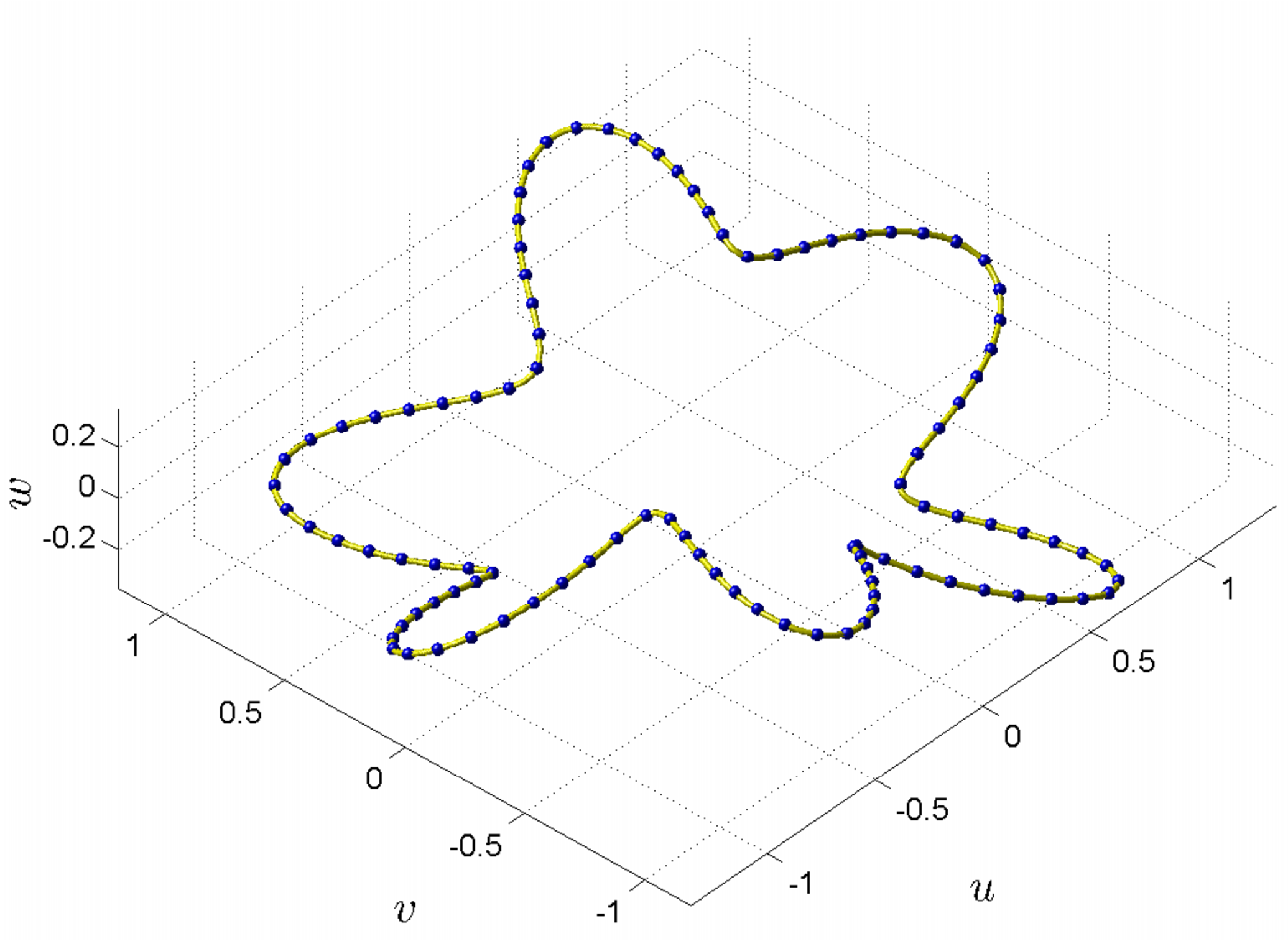
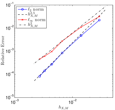
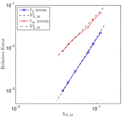
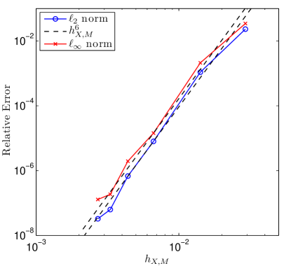
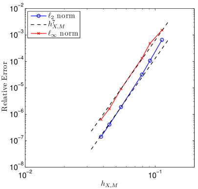
We provide numerical results verifying Theorems 10 and 14 for target functions inside and outside of the native space, respectively. Two different compact embedded smooth submanifolds in 3superscript3\mathbb{R}^{3} are considered. The first is a one-dimensional submanifold with the parametric representation

𝕄1={(u,v,w)3|u=(1+13cos6θ)cosθ,v=(1+13cos6θ)sinθ,w=13sin2θ, 0θ<2π}.subscript𝕄1conditional-set𝑢𝑣𝑤superscript3formulae-sequence𝑢1136𝜃𝜃formulae-sequence𝑣1136𝜃𝜃formulae-sequence𝑤132𝜃 0𝜃2𝜋\mathbb{M}_{1}=\left\{(u,v,w)\in\mathbb{R}^{3}\;\left|\;u=\left(1+\frac{1}{3}\cos 6\theta\right)\cos\theta,\;v=\left(1+\frac{1}{3}\cos 6\theta\right)\sin\theta,\;w=\frac{1}{3}\sin 2\theta,\;0\leq\theta<2\pi\right.\right\}. (5)

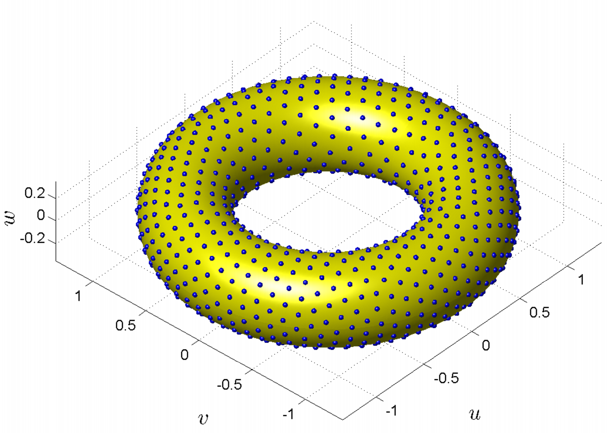
This curve is displayed in Figure 1. The second submanifold is a two-dimensional torus with parametric representation

𝕄2={(u,v,w)3|u=(1+13cosλ)cosθ,v=(1+13cosλ)sinθ,w=13sinλ, 0θ,λ<2π}.subscript𝕄2conditional-set𝑢𝑣𝑤superscript3formulae-sequence𝑢113𝜆𝜃formulae-sequence𝑣113𝜆𝜃formulae-sequence𝑤13𝜆formulae-sequence 0𝜃𝜆2𝜋\mathbb{M}_{2}=\left\{(u,v,w)\in\mathbb{R}^{3}\;\left|\;u=\left(1+\frac{1}{3}\cos\lambda\right)\cos\theta,\;v=\left(1+\frac{1}{3}\cos\lambda\right)\sin\theta,\;w=\frac{1}{3}\sin\lambda,\;0\leq\theta,\lambda<2\pi\right.\right\}. (6)

This torus is displayed in Figure 1.

Refer to caption
Refer to caption
Figure 1: Compact embedded smooth submanifolds used for the numerical experiments. (a) One-dimensional curve 𝕄1subscript𝕄1\mathbb{M}_{1} described parametrically by (5). (b) Two-dimensional torus 𝕄2subscript𝕄2\mathbb{M}_{2} described parametrically by (6). Solid spheres mark the locations of the near-minimum Reisz energy interpolation nodes for (a) N=100𝑁100N=100 and (b) N=1000𝑁1000N=1000.

To discretize 𝕄1subscript𝕄1\mathbb{M}_{1} and 𝕄2subscript𝕄2\mathbb{M}_{2}, we use a hierarchy of node sets with increasing cardinalities. For 𝕄1subscript𝕄1\mathbb{M}_{1} we use cardinalities of N=50𝑁50N=50, 100100100, 200200200, 300300300, 400400400, and 500500500, while for 𝕄2subscript𝕄2\mathbb{M}_{2} we use N=500𝑁500N=500, 750750750, 100010001000, 200020002000, 300030003000, and 400040004000. The node sets for both manifolds are obtained by arranging the nodes so that their Reisz energy (with a power of 2) is near minimal as described in Hardin and Saff’s seminal article [19]. For 𝕄1subscript𝕄1\mathbb{M}_{1}, this results in node sets with mesh norms hX,𝕄1subscript𝑋subscript𝕄1h_{X,\mathbb{M}_{1}} that decrease like 1/N1𝑁1/N, while the mesh norms hX,𝕄2subscript𝑋subscript𝕄2h_{X,\mathbb{M}_{2}} for 𝕄2subscript𝕄2\mathbb{M}_{2} decrease like 1/N1𝑁1/\sqrt{N}. Additionally, the mesh ratios ρX,𝕄1subscript𝜌𝑋subscript𝕄1\rho_{X,\mathbb{M}_{1}} and ρX,𝕄2subscript𝜌𝑋subscript𝕄2\rho_{X,\mathbb{M}_{2}} remain roughly constant. The small solid spheres on the curve in Figure 1 display the node locations for the N=100𝑁100N=100 node set, while the small spheres on the torus in Figure 1 display the N=1000𝑁1000N=1000 node set. It is obvious from the latter plot that the nodes are not oriented along any vertices or lines emphasizing the ability of the proposed kernel interpolation technique to handle arbitrary node layouts on a submanifold.

The positive definite kernel we use for constructing the interpolants in the experiments is Wendland’s compactly supported RBF

ϕ3,2(x,y)=ϕ3,2(xy)=ϕ3,2(r)=(1rδ)+6(3+18rδ+35(rδ)2),subscriptitalic-ϕ32𝑥𝑦subscriptitalic-ϕ32norm𝑥𝑦subscriptitalic-ϕ32𝑟superscriptsubscript1𝑟𝛿6318𝑟𝛿35superscript𝑟𝛿2\phi_{3,2}(x,y)=\phi_{3,2}(\|x-y\|)=\phi_{3,2}(r)=\left(1-\dfrac{r}{\delta}\right)_{+}^{6}\left(3+18\dfrac{r}{\delta}+35\left(\dfrac{r}{\delta}\right)^{2}\right), (7)

which is positive definite in 3superscript3\mathbb{R}^{3} and has 4 continuous derivatives [44, §9.4]. Furthermore, the native space of this kernel is known to be H4(3)superscript𝐻4superscript3H^{4}(\mathbb{R}^{3}) [44, p.157], which means τ=4𝜏4\tau=4 in Theorems 10 and 14. According to Theorem 5, the native spaces on 𝕄1subscript𝕄1\mathbb{M}_{1} and 𝕄2subscript𝕄2\mathbb{M}_{2} for this kernel are thus H3(𝕄1)superscript𝐻3subscript𝕄1H^{3}(\mathbb{M}_{1}) and H3.5(𝕄2)superscript𝐻3.5subscript𝕄2H^{3.5}(\mathbb{M}_{2}). The free parameter δ𝛿\delta is referred to as the support radius and its optimal value depends on numerous factors which are neither easy nor obvious to determine (cf.  [44, Ch. 15] or [20, Ch. 5]). Since our intention in the present study is only to provide verification of the error estimates presented above, we set δ=8/3𝛿83\delta=8/3 (the maximum distance of any two nodes on either 𝕄1subscript𝕄1\mathbb{M}_{1} or 𝕄2subscript𝕄2\mathbb{M}_{2}) for all the numerical results and leave investigations of selecting δ𝛿\delta for interpolation on submanifolds to a separate study.

One difficulty with verifying error estimates of the type given in Theorems 10 and 14 is coming up with explicit forms of target functions belonging to a desired Sobolev space. Fortunately, Sobolev spaces can be defined in terms of decay rates of Fourier transforms [44, p. 133]. Using this definition, a straightforward calculation shows any function κd𝜅superscript𝑑\kappa\in\mathbb{R}^{d} whose Fourier transform satisfies

κ^(ξ)(1+ξ22)νsimilar-to^𝜅𝜉superscript1superscriptsubscriptnorm𝜉22𝜈\widehat{\kappa}(\xi)\sim(1+\|\xi\|_{2}^{2})^{-\nu} (8)

belongs to every Sobolev space Hβ(d)superscript𝐻𝛽superscript𝑑H^{\beta}(\mathbb{R}^{d}), with β<2νd/2𝛽2𝜈𝑑2\beta<2\nu-d/2. Thus, we can use functions whose Fourier transforms satisfy (8) with ν=(β+d/2)/2𝜈𝛽𝑑22\nu=(\beta+d/2)/2 as target functions since they will then be in Hs(𝕄)superscript𝐻𝑠𝕄H^{s}(\mathbb{M}) for all s<β(dk)/2𝑠𝛽𝑑𝑘2s<\beta-(d-k)/2.

A well-known class of functions that satisfy (8) (with strict equality) are the Matérn kernels [25] or Sobolev splines and are defined as

κν(x,y)=κν(xy)=κν(r)=21(νd/2)Γ(νd/2)rνd/2Kνd/2(r),ν>d/2formulae-sequencesubscript𝜅𝜈𝑥𝑦subscript𝜅𝜈norm𝑥𝑦subscript𝜅𝜈𝑟superscript21𝜈𝑑2Γ𝜈𝑑2superscript𝑟𝜈𝑑2subscript𝐾𝜈𝑑2𝑟𝜈𝑑2\kappa_{\nu}(x,y)=\kappa_{\nu}(\|x-y\|)=\kappa_{\nu}(r)=\frac{2^{1-(\nu-d/2)}}{\Gamma(\nu-d/2)}r^{\nu-d/2}K_{\nu-d/2}(r),\;\nu>d/2

where Kνd/2subscript𝐾𝜈𝑑2K_{\nu-d/2} corresponds to the K𝐾K-Bessel function of order νd/2𝜈𝑑2\nu-d/2. To generate interesting target functions for verifying Theorems 10 and 14, we use linear combinations of these Matérn kernels as follows. Let X={x1,x2,,xm}𝑋subscript𝑥1subscript𝑥2subscript𝑥𝑚X=\{x_{1},x_{2},\ldots,x_{m}\} be some set of distinct points on the submanifold under consideration (either 𝕄1subscript𝕄1\mathbb{M}_{1} or 𝕄2subscript𝕄2\mathbb{M}_{2}), then the target function is given by

fβ(x)=j=1mcjκ12(β+d/2)(xxj).subscript𝑓𝛽𝑥superscriptsubscript𝑗1𝑚subscript𝑐𝑗subscript𝜅12𝛽𝑑2norm𝑥subscript𝑥𝑗f_{\beta}(x)=\sum_{j=1}^{m}c_{j}\kappa_{\frac{1}{2}(\beta+d/2)}(\|x-x_{j}\|). (9)

The coefficients c1,c2,,cmsubscript𝑐1subscript𝑐2subscript𝑐𝑚c_{1},c_{2},\ldots,c_{m} are determined by the requiring fβsubscript𝑓𝛽f_{\beta} interpolate the following function at the points in X𝑋X:

p(x)=18(u510u3v2+5uv4)(u2+v260w2),𝑝𝑥18superscript𝑢510superscript𝑢3superscript𝑣25𝑢superscript𝑣4superscript𝑢2superscript𝑣260superscript𝑤2p(x)=\frac{1}{8}\left(u^{5}-10u^{3}v^{2}+5uv^{4}\right)\left(u^{2}+v^{2}-60w^{2}\right), (10)

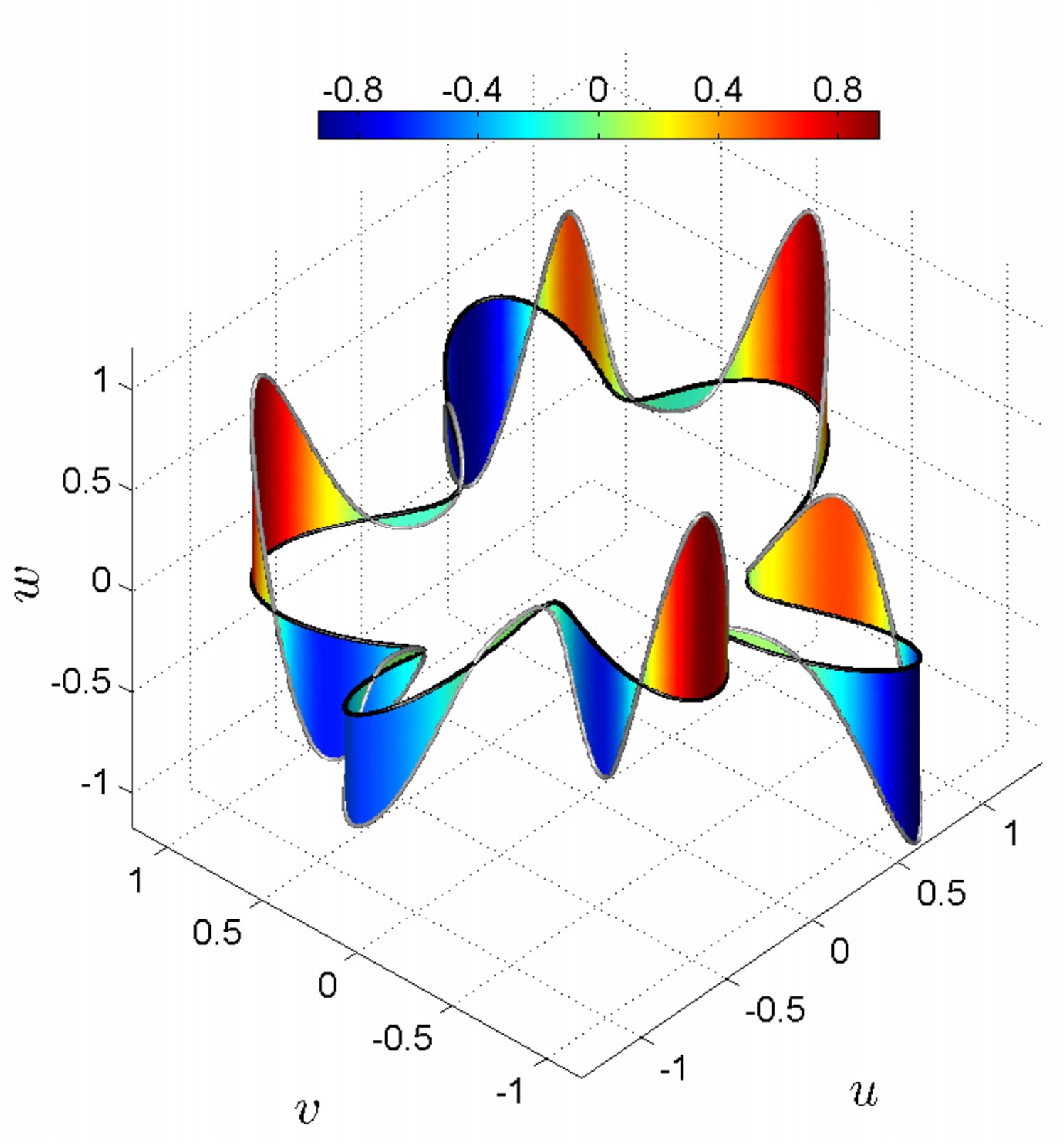
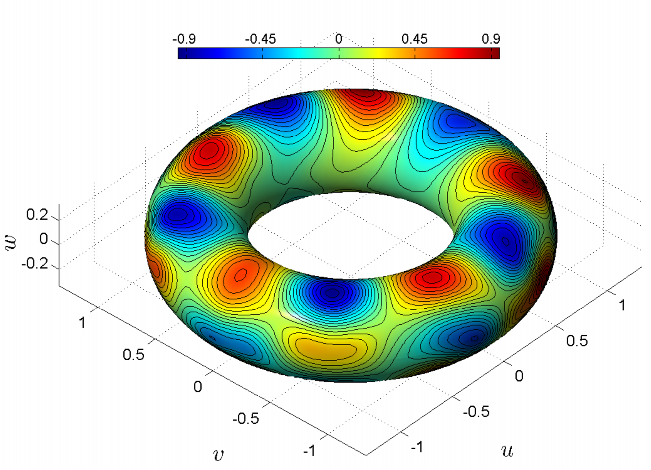
where u𝑢u, v𝑣v, and w𝑤w are the components of x𝑥x. For 𝕄1subscript𝕄1\mathbb{M}_{1}, we use m=25𝑚25m=25 quasi-minimum Reisz energy points for X𝑋X, while for 𝕄2subscript𝕄2\mathbb{M}_{2} we use n=100𝑛100n=100 quasi-minimum Reisz energy points. Plots of the target function for β=4𝛽4\beta=4 are displayed in Figure 2(a) and (b) for 𝕄1subscript𝕄1\mathbb{M}_{1} and 𝕄2subscript𝕄2\mathbb{M}_{2}, respectively. Note that fβsubscript𝑓𝛽f_{\beta} is not the kernel interpolant to be compared against the theoretical error estimates, rather it is the form of the target functions to be interpolated.
Refer to caption
Refer to caption
Figure 2: Visualization of two of the target functions for the numerical experiments. (a) The target function (9) for 𝕄1subscript𝕄1\mathbb{M}_{1} with m=25𝑚25m=25 and β=4𝛽4\beta=4 displayed as the height above the submanifold (i.e. (u,v,w+f4(x))𝑢𝑣𝑤subscript𝑓4𝑥(u,v,w+f_{4}(x))) together with colors indicating the values of the function. (b) The target function for 𝕄2subscript𝕄2\mathbb{M}_{2} with m=100𝑚100m=100 and β=4𝛽4\beta=4 with colors corresponding to the values of the target function on the submanifold and black lines corresponding to contours of the function.

In the results below, the errors are measured by evaluating the kernel interpolants and the target functions at a much denser set of points that sufficiently cover the manifolds. For 𝕄1subscript𝕄1\mathbb{M}_{1}, P=3000𝑃3000P=3000 evaluation points are used, while P=24,300𝑃24300P=24,300 points are used for 𝕄2subscript𝕄2\mathbb{M}_{2}. We approximate the (relative) L2(𝕄)subscript𝐿2𝕄L_{2}(\mathbb{M})-norms of the errors by approximating the surface integrals over the manifolds using a midpoint-type rule. We use the following abuse of notation to denote the approximate L2(𝕄)subscript𝐿2𝕄L_{2}(\mathbb{M})-norm:

fL2(𝕄):=(𝕄[f(x)]2𝑑x)1/2(i=1Pwi[f(xi)]2)1/2:=f2(𝕄),assignsubscriptnorm𝑓subscript𝐿2𝕄superscriptsubscript𝕄superscriptdelimited-[]𝑓𝑥2differential-d𝑥12superscriptsuperscriptsubscript𝑖1𝑃subscript𝑤𝑖superscriptdelimited-[]𝑓subscript𝑥𝑖212assignsubscriptnorm𝑓subscript2𝕄\|f\|_{L_{2}(\mathbb{M})}:=\left(\int_{\mathbb{M}}[f(x)]^{2}dx\right)^{1/2}\approx\left(\sum_{i=1}^{P}w_{i}[f(x_{i})]^{2}\right)^{1/2}:=\|f\|_{\ell_{2}(\mathbb{M})},

where {wi}i=1Psuperscriptsubscriptsubscript𝑤𝑖𝑖1𝑃\{w_{i}\}_{i=1}^{P} are quadrature weights for the evaluation points {xi}i=1Psuperscriptsubscriptsubscript𝑥𝑖𝑖1𝑃\{x_{i}\}_{i=1}^{P} on the manifold. We also meausure the max-norm errors over the manifolds. We use the standard definition for this norm and denote it with the standard notation of (𝕄)subscript𝕄\ell_{\infty}(\mathbb{M}).

Refer to caption
(a) 𝕄1subscript𝕄1\mathbb{M}_{1}, β=4𝛽4\beta=4
Refer to caption
(b) 𝕄2subscript𝕄2\mathbb{M}_{2}, β=4𝛽4\beta=4
Refer to caption
(c) 𝕄1subscript𝕄1\mathbb{M}_{1}, β=3.5𝛽3.5\beta=3.5
Refer to caption
(d) 𝕄2subscript𝕄2\mathbb{M}_{2}, β=3.5𝛽3.5\beta=3.5
Figure 3: Relative errors in reconstructing the different target functions fβsubscript𝑓𝛽f_{\beta} in (9) on the two different submanifolds with the kernel (7). Plots in (a) and (c) are for 𝕄1subscript𝕄1\mathbb{M}_{1} and plots in (b) and (d) are for M2subscript𝑀2M_{2}. Lines marked with open circles in each figure correspond to the relative 2(𝕄)subscript2𝕄\ell_{2}(\mathbb{M}) error and lines marked with x’s are for the relative (𝕄)subscript𝕄\ell_{\infty}(\mathbb{M}) errors. In (a) and (b) the dashed and dashed-dotted lines correspond to the predicted error estimates from Theorem 10 for 2(𝕄)subscript2𝕄\ell_{2}(\mathbb{M}) and (𝕄)subscript𝕄\ell_{\infty}(\mathbb{M}), respectively, while these lines in (c) and (d) correspond to the predicted estimates from Theorem 14.

For the first numerical experiment, we set set β=4𝛽4\beta=4 in (9) for 𝕄1subscript𝕄1\mathbb{M}_{1} and 𝕄2subscript𝕄2\mathbb{M}_{2}. Since the native space for the kernel (7) is H4(3)superscript𝐻4superscript3H^{4}(\mathbb{R}^{3}), we expect the estimates from Theorem 10 to apply for these target functions. According to this theorem, the 2subscript2\ell_{2} errors for 𝕄1subscript𝕄1\mathbb{M}_{1} and 𝕄2subscript𝕄2\mathbb{M}_{2} should decrease like hX,𝕄13superscriptsubscript𝑋subscript𝕄13h_{X,\mathbb{M}_{1}}^{3} and hX,𝕄23.5superscriptsubscript𝑋subscript𝕄23.5h_{X,\mathbb{M}_{2}}^{3.5}, while the subscript\ell_{\infty} errors should decrease like hX,𝕄12.5superscriptsubscript𝑋subscript𝕄12.5h_{X,\mathbb{M}_{1}}^{2.5} and hX,𝕄22.5superscriptsubscript𝑋subscript𝕄22.5h_{X,\mathbb{M}_{2}}^{2.5}. Figures 3(a) and (b) display the computed relative errors versus the mesh norm for f4subscript𝑓4f_{4} together with the predicted estimates. The figures show good agreement between the numerical and theoretical results.

In the second experiment, we set β=3.5𝛽3.5\beta=3.5 in (9) for 𝕄1subscript𝕄1\mathbb{M}_{1} and 𝕄2subscript𝕄2\mathbb{M}_{2}, which makes the target functions rougher than the native space of the kernel and means the estimates from Theorem 14 will apply. Assuming the mesh ratio is roughly constant (which is true for our experiments), this theorem predicts that the 2subscript2\ell_{2} errors for 𝕄1subscript𝕄1\mathbb{M}_{1} and 𝕄2subscript𝕄2\mathbb{M}_{2} should decrease like hX,𝕄12.5superscriptsubscript𝑋subscript𝕄12.5h_{X,\mathbb{M}_{1}}^{2.5} and hX,𝕄23superscriptsubscript𝑋subscript𝕄23h_{X,\mathbb{M}_{2}}^{3}, while the subscript\ell_{\infty} errors should decrease like hX,𝕄12superscriptsubscript𝑋subscript𝕄12h_{X,\mathbb{M}_{1}}^{2} and hX,𝕄22superscriptsubscript𝑋subscript𝕄22h_{X,\mathbb{M}_{2}}^{2}. Similar to the previous experiment, Figures 3(c) and (d) display the computed relative errors for these target functions together with the predicted estimates. Good agreement between the numerical and theoretical results is again displayed.

As a final numerical experiment, we verify the “doubling” estimates from Corollary 12. For the target function we use (10) directly. This function is C(3)superscript𝐶superscript3C^{\infty}(\mathbb{R}^{3}) and is thus much smoother than the native space of the kernel (7). According to Corollary 12, the 2subscript2\ell_{2} errors for 𝕄1subscript𝕄1\mathbb{M}_{1} and 𝕄2subscript𝕄2\mathbb{M}_{2} should decrease like hX,𝕄16superscriptsubscript𝑋subscript𝕄16h_{X,\mathbb{M}_{1}}^{6} and hX,𝕄27superscriptsubscript𝑋subscript𝕄27h_{X,\mathbb{M}_{2}}^{7} for this target function and kernel. Figure 4(a) and (b) displays the results for 𝕄1subscript𝕄1\mathbb{M}_{1} and 𝕄2subscript𝕄2\mathbb{M}_{2}, respectively. We again find good agreement between the numerical and theoretical results. The results from the figure also indicate that there does not appear to be a reduction in the estimates for the subscript\ell_{\infty} error for this case.

Refer to caption
(a) 𝕄1subscript𝕄1\mathbb{M}_{1}
Refer to caption
(b) 𝕄2subscript𝕄2\mathbb{M}_{2}
Figure 4: Relative errors in reconstructing the target function (10) on (a) 𝕄1subscript𝕄1\mathbb{M}_{1} and (b) 𝕄2subscript𝕄2\mathbb{M}_{2} with the kernel (7). The dashed lines in the figure correspond to the predicted error estimates for the 2(𝕄)subscript2𝕄\ell_{2}(\mathbb{M}) error from Corollary 12.

Acknowledgments. We wish to express our deep gratitude to Drs. Douglas Hardin and Edward Saff and Ms. Ayla Gafni, all from Vanderbilt University, for providing us with the near-minimum Reisz energy points for the torus used in the numerical experiments.

References

  • [1] D. Adalsteinsson and J. A. Sethian. Transport and diffusion of material quantities on propagating interfaces via level set methods. J. Comput. Phys., 185(1):271–288, 2003.
  • [2] R. A. Adams. Sobolev spaces. Academic Press [A subsidiary of Harcourt Brace Jovanovich, Publishers], New York-London, 1975. Pure and Applied Mathematics, Vol. 65.
  • [3] P. Alfeld, M. Neamtu, and L. L. Schumaker. Fitting scattered data on sphere-like surfaces using spherical splines. J. Comput. Appl. Math., 73(1-2):5–43, 1996.
  • [4] C. L. Bajaj, F. Bernardini, and G. Xu. Automatic reconstruction of surfaces and scalar fields from 3D scans. In SIGGRAPH ’95: Proceedings of the 22nd annual conference on Computer graphics and interactive techniques, pages 109–118, New York, NY, USA, 1995. ACM.
  • [5] R. E. Barnhill and H. S. Ou. Surfaces defined on surfaces. Comput. Aided Geom. Des., 7(1-4):323–336, 1990.
  • [6] M. Belkin and P. Niyogi. Semi-supervised learning on riemannian manifolds. Mach. Learn., 56:209–239, 2004.
  • [7] O. V. Besov, V. P. Ilin, and S. M. Nikolskiĭ. Integral representations of functions and imbedding theorems. Vol. II. V. H. Winston & Sons, Washington, D.C., 1979. Scripta Series in Mathematics, Edited by Mitchell H. Taibleson.
  • [8] D. A. Calhoun and C. Helzel. A finite volume method for solving parabolic equations on logically Cartesian curved surface meshes. SIAM Journal on Scientific Computing, 31(6):4066–4099, 2009.
  • [9] U. Clarenz, U. Diewald, and M. Rumpf. Anisotropic geometric diffusion in surface processing. In VISUALIZATION ’00: Proceedings of the 11th IEEE Visualization 2000 Conference (VIS 2000), Washington, DC, USA, 2000. IEEE Computer Society.
  • [10] O. Davydov and L. L. Schumaker. Scattered data fitting on surfaces using projected powell-sabin splines. In Proceedings of the 12th IMA international conference on Mathematics of surfaces XII, pages 138–153, Berlin, Heidelberg, 2007. Springer-Verlag.
  • [11] M. Desbrun, M. Meyer, P. Schröder, and A. H. Barr. Implicit fairing of irregular meshes using diffusion and curvature flow. In SIGGRAPH ’99: Proceedings of the 26th annual conference on Computer graphics and interactive techniques, pages 317–324, New York, NY, USA, 1999. ACM Press/Addison-Wesley Publishing Co.
  • [12] W. Erb and F. Filbir. Approximation by positive definite functions on compact groups. Numer. Funct. Anal. Optim., 29(9-10):1082–1107, 2008.
  • [13] J. C. Ferreira and V. A. Menegatto. Eigenvalues of integral operators defined by smooth positive definite kernels. Integral Equations Operator Theory, 64(1):61–81, 2009.
  • [14] F. Filbir and D. Schmid. Stability results for approximation by positive definite functions on SO(3)SO3{\rm SO}(3). J. Approx. Theory, 153(2):170–183, 2008.
  • [15] N. Flyer and G. B. Wright. A radial basis function method for the shallow water equations on a sphere. Proc. Roy. Soc. A, 465:1949–1976, 2009.
  • [16] T. A. Foley, D. A. Lane, G. M. Nielson, R. Franke, and H. Hagen. Interpolation of scattered data on closed surfaces. Comput. Aided Geom. Des., 7(1-4):303–312, 1990.
  • [17] E. J. Fuselier and G. B. Wright. Stability and error estimates for vector field interpolation and decomposition on the sphere with rbfs. SIAM J. Numer. Anal., 47(5):3213–3239, 2009.
  • [18] T. Hangelbroek, F. Narcowich, and J. Ward. Kernel approximation on manifolds I: Bounding the lebesgue constant. To appear in SIAM J. on Math. Anal., (2010), http://arxiv.org/abs/0909.0033v2.
  • [19] D. P. Hardin and E. B. Saff. Discretizing manifolds via minimum energy points. Notices Amer. Math. Soc., 51:1186–1194, 2004.
  • [20] A. Iske. Multiresolution Methods in Scattered Data Modelling. Springer-Verlag, Heidelberg, 2004.
  • [21] J. M. Lee. Introduction to smooth manifolds, volume 218 of Graduate Texts in Mathematics. Springer-Verlag, New York, 2003.
  • [22] J. Levesley and D. L. Ragozin. Radial basis interpolation on homogeneous manifolds: convergence rates. Adv. Comput. Math., 27(2):237–246, 2007.
  • [23] J.-L. Lions and E. Magenes. Problemi ai limiti non omogenei. III. Ann. Scuola Norm. Sup. Pisa (3), 15:41–103, 1961.
  • [24] W. R. Madych and S. A. Nelson. Multivariate interpolation and conditionally positive definite functions. Approx. Theory Appl., 4(4):77–89, 1988.
  • [25] B. Matérn. Spatial variation, volume 36 of Lecture Notes in Statistics. Springer-Verlag, Berlin, second edition, 1986. With a Swedish summary.
  • [26] T. M. Morton and M. Neamtu. Error bounds for solving pseudodifferential equations on spheres by collocation with zonal kernels. J. Approx. Theory, 144(2):242–268, 2002.
  • [27] F. J. Narcowich. Generalized Hermite interpolation and positive definite kernels on a Riemannian manifold. J. Math. Anal. Appl., 190(1):165–193, 1995.
  • [28] F. J. Narcowich. Recent developments in error estimates for scattered-data interpolation via radial basis functions. Numer. Algorithms, 39(1-3):307–315, 2005.
  • [29] F. J. Narcowich, X. Sun, and J. D. Ward. Approximation power of RBFs and their associated SBFs: a connection. Adv. Comput. Math., 27(1):107–124, 2007.
  • [30] F. J. Narcowich, X. Sun, J. D. Ward, and H. Wendland. Direct and inverse Sobolev error estimates for scattered data interpolation via spherical basis functions. Found. Comput. Math., 7(3):369–390, 2007.
  • [31] F. J. Narcowich and J. D. Ward. Generalized Hermite interpolation via matrix-valued conditionally positive definite functions. Math. Comp., 63(208):661–687, 1994.
  • [32] F. J. Narcowich, J. D. Ward, and H. Wendland. Sobolev bounds on functions with scattered zeros, with applications to radial basis function surface fitting. Math. Comp., 74(250):743–763 (electronic), 2005.
  • [33] F. J. Narcowich, J. D. Ward, and H. Wendland. Sobolev error estimates and a Bernstein inequality for scattered data interpolation via radial basis functions. Constr. Approx., 24(2):175–186, 2006.
  • [34] M. Neamtu. Splines on surfaces. In Handbook on CAGD, pages 229–253. North-Holland, Amsterdam, 2002.
  • [35] I. L. Novak, F. Gao, Y.-S. Choi, D. Resasco, J. C. Schaff, and B. M. Slepchenko. Diffusion on a curved surface coupled to diffusion in the volume: Application to cell biology. J. Comput. Phys., 226(2):1271–1290, 2007.
  • [36] D. L. Ragozin and J. Levesley. The density of translates of zonal kernels on compact homogeneous spaces. J. Approx. Theory, 103(2):252–268, 2000.
  • [37] I. F. Sbalzarini, A. Hayer, A. Helenius, and P. Koumoutsakos. Simulations of (an)isotropic diffusion on curved biological surfaces. Biophys. J., 90:878–885, 2006.
  • [38] R. Schaback. Improved error bounds for scattered data interpolation by radial basis functions. Math. Comput., 68(225):201–216, 1999.
  • [39] R. Schaback. Native Hilbert spaces for radial basis functions. I. In New developments in approximation theory (Dortmund, 1998), volume 132 of Internat. Ser. Numer. Math., pages 255–282. Birkhäuser, Basel, 1999.
  • [40] R. Schaback. A unified theory of radial basis functions. Native Hilbert spaces for radial basis functions. II. J. Comput. Appl. Math., 121(1-2):165–177, 2000. Numerical analysis in the 20th century, Vol. I, Approximation theory.
  • [41] P. Schwartz, D. Adalsteinsson, P. Colella, A. P. Arkin, and M. Onsum. Numerical computation of diffusion on a surface. Proc. Nat. Acad. Sci., 102(32):11151–11156, 2005.
  • [42] J. Stam. Flows on surfaces of arbitrary topology. In SIGGRAPH ’03: ACM SIGGRAPH 2003 Papers, pages 724–731, New York, NY, USA, 2003. ACM.
  • [43] J. Stewart. Positive definite functions and generalizations, an historical survey. Rocky Mountain J. Math., 6(3):409–434, 1976.
  • [44] H. Wendland. Scattered data approximation, volume 17 of Cambridge Monographs on Applied and Computational Mathematics. Cambridge University Press, Cambridge, 2005.
  • [45] Z. M. Wu. Hermite-Birkhoff interpolation of scattered data by radial basis functions. Approx. Theory Appl., 8(2):1–10, 1992.
  • [46] W. zu Castell and F. Filbir. Radial basis functions and corresponding zonal series expansions on the sphere. J. Approx. Theory, 134(1):65–79, 2005.
  • [47] W. zu Castell and F. Filbir. Strictly positive definite functions on generalized motion groups. In Algorithms for approximation, pages 349–357. Springer, Berlin, 2007.