On Compound Poisson Processes Arising in
Change-Point Type Statistical Models
as Limiting Likelihood Ratios

Abstract

Different change-point type models encountered in statistical inference for stochastic processes give rise to different limiting likelihood ratio processes. In a previous paper of one of the authors it was established that one of these likelihood ratios, which is an exponential functional of a two-sided Poisson process driven by some parameter, can be approximated (for sufficiently small values of the parameter) by another one, which is an exponential functional of a two-sided Brownian motion. In this paper we consider yet another likelihood ratio, which is the exponent of a two-sided compound Poisson process driven by some parameter. We establish, that similarly to the Poisson type one, the compound Poisson type likelihood ratio can be approximated by the Brownian type one for sufficiently small values of the parameter. We equally discuss the asymptotics for large values of the parameter and illustrate the results by numerical simulations.

Keywords: compound Poisson process, non-regularity, change-point, limiting likelihood ratio process, Bayesian estimators, maximum likelihood estimator, limiting distribution, limiting mean squared error, asymptotic relative efficiency

Mathematics Subject Classification (2000): 62F99, 62M99

1 Introduction

In this work we are interested by the asymptotic study of non-regular parametric statistical models encountered in statistical inference for stochastic processes. An exhaustive exposition of the parameter estimation theory in both regular and non-regular cases is given in the classical book [15] by Ibragimov and Khasminskii. They have developed a general theory of estimation based on the analysis of renormalized likelihood ratio. Their approach consists in proving first that the renormalized likelihood ratio (with a properly chosen renormalization rate) weekly converges to some non-degenerate limit: the limiting likelihood ratio process. Thereafter, the properties of the estimators (namely their rate of convergence and limiting distributions) are deduced. Finally, based on the estimators, one can also construct confidence intervals, tests, and so on. Note that this approach also provides the convergence of moments, allowing one to deduce equally the asymptotics of some statistically important quantities, such as the mean squared errors of the estimators.

It is well known that in the regular case the limiting likelihood ratio is given by the LAN property and is the same for different models (the renormalization rate being usually $1/\sqrt{n}\,$). So, the classical estimators — the maximum likelihood estimator and the Bayesian estimators — are consistent, asymptotically normal (usually with rate $1/\sqrt{n}\,$) and asymptotically efficient.

In non-regular cases the situation essentially changes: the renormalization rate is usually better (for example, $1/n$ in change-point type models), but the limiting likelihood ratio can be different in different models. So, the classical estimators are still consistent, but may have different limiting distributions (though with a better rate) and, in general, only the Bayesian estimators are asymptotically efficient.

In [7] a relation between two different limiting likelihood ratios arising in change-point type models was established by one of the authors. More precisely, it was shown that the first one, which is an exponential functional of a two-sided Poisson process driven by some parameter, can be approximated (for sufficiently small values of the parameter) by the second one, defined by

$$Z_{0}(x)=\exp\left\{W(x)-\frac{1}{2}\left|x\right|\right\},\quad x\in\mathbb{R},$$ (1)

where $W$ is a standard two-sided Brownian motion. In this paper we consider yet another limiting likelihood ratio process arising in change-point type models and show that it is related to $Z_{0}$ in a similar way.

The process $Z_{\gamma,f}$

We introduce the random process $Z_{\gamma,f}$ on $\mathbb{R}$ as the exponent of a two-sided compound Poisson process given by

$$\ln Z_{\gamma,f}(x)=\begin{cases}\vphantom{{\mathchoice{\mbox{$\displaystyle\left)\vrule height=14.5pt,depth=0.0pt,width=0.0pt\right.\n@space$}}{\mbox{$\textstyle\left)\vrule height=14.5pt,depth=0.0pt,width=0.0pt\right.\n@space$}}{\mbox{$\scriptstyle\left)\vrule height=7.10497pt,depth=0.0pt,width=0.0pt\right.\n@space$}}{\mbox{$\scriptscriptstyle\left)\vrule height=3.625pt,depth=0.0pt,width=0.0pt\right.\n@space$}}}}\sum_{k=1}^{\Pi_{+}(x)}\ln\frac{f(\varepsilon_{k}^{+}+\gamma)}{f(\varepsilon_{k}^{+})}\,,&\text{if }x\geqslant 0,\\ \vphantom{{\mathchoice{\mbox{$\displaystyle\left)\vrule height=14.5pt,depth=0.0pt,width=0.0pt\right.\n@space$}}{\mbox{$\textstyle\left)\vrule height=14.5pt,depth=0.0pt,width=0.0pt\right.\n@space$}}{\mbox{$\scriptstyle\left)\vrule height=7.10497pt,depth=0.0pt,width=0.0pt\right.\n@space$}}{\mbox{$\scriptscriptstyle\left)\vrule height=3.625pt,depth=0.0pt,width=0.0pt\right.\n@space$}}}}\sum_{k=1}^{\Pi_{-}(-x)}\ln\frac{f(\varepsilon_{k}^{-}-\gamma)}{f(\varepsilon_{k}^{-})}\,,&\text{if }x\leqslant 0,\\ \end{cases}$$ (2)

where $\gamma>0$, $f$ is a strictly positive density of some random variable $\varepsilon$ with mean $0$ and variance $1$, $\Pi_{+}$ and $\Pi_{-}$ are two independent Poisson processes of intensity $1$ on $\mathbb{R}_{+}$, $\varepsilon_{k}^{\pm}$ are independent random variables with density $f$ which are also independent of $\Pi_{\pm}$, and we use the convention $\sum_{k=1}^{0}a_{k}=0$. We equally introduce the random variables

$$\zeta_{\gamma,f} =\frac{\int_{\mathbb{R}}x\,Z_{\gamma,f}(x)\;dx}{\int_{\mathbb{R}}\,Z_{\gamma,f}(x)\;dx}\,,$$ (3)

$$\xi_{\gamma,f}^{-} =\inf\Bigl{\{}z:Z_{\gamma,f}(z)=\sup_{x\in\mathbb{R}}Z_{\gamma,f}(x)\Bigr{\}},$$

$$\xi_{\gamma,f}^{+} =\sup\Bigl{\{}z:Z_{\gamma,f}(z)=\sup_{x\in\mathbb{R}}Z_{\gamma,f}(x)\Bigr{\}},$$

$$\xi_{\gamma,f}^{\alpha} =\alpha\,\xi_{\gamma,f}^{-}+(1-\alpha)\,\xi_{\gamma,f}^{+},\quad\alpha\in[0,1],$$

related to this process, as well as their second moments $B_{\gamma,f}=\mathbf{E}\zeta_{\gamma,f}^{2}$ and $M_{\gamma,f}^{\alpha}=\mathbf{E}(\xi_{\gamma,f}^{\alpha})^{2}$.

An important particular case of this process is the one where the density $f$ is Gaussian, that is, $\varepsilon\sim\mathcal{N}(0,1)$. In this case we will omit the index $f$ and write $Z_{\gamma}$ instead of $Z_{\gamma,f}$, $\xi_{\gamma}^{\alpha}$ instead of $\xi_{\gamma,f}^{\alpha}$, and so on. Note that since

$$\ln\frac{f(\varepsilon\pm\gamma)}{f(\varepsilon)}=\mp\gamma\varepsilon-\frac{\gamma^{2}}{2}\sim\mathcal{N}(-\gamma^{2}/2,\gamma^{2}),$$

the process $Z_{\gamma}$ is symmetric and has Gaussian jumps.

The process $Z_{\gamma,f}$, up to a linear time change, arises in some non-regular, namely change-point type, statistical models as the limiting likelihood ratio process, and the variables $\zeta_{\gamma,f}$ and $\xi_{\gamma,f}^{\alpha}$ as the limiting distributions of the Bayesian estimators and of the appropriately chosen maximum likelihood estimator, respectively. The maximum likelihood estimator being not unique in the underlying models, the appropriate choice here is a linear combination with weights $\alpha$ and $1-\alpha$ of its minimal and maximal values. Moreover, the quantities $B_{\gamma,f}$ and $M_{\gamma,f}^{\alpha}$ are the limiting mean squared errors (sometimes also called limiting variances) of these estimators and, the Bayesian estimators being asymptotically efficient, the ratio $E_{\gamma,f}^{\alpha}=B_{\gamma,f}/M_{\gamma,f}^{\alpha}$ is the asymptotic relative efficiency of this maximum likelihood estimator.

The examples include the two-phase regression model and the threshold autoregressive (TAR) model. The linear case of the former was studied by Koul and Qian in [16], while the non-linear one was investigated by Ciuperca in [6]. Concerning the TAR model, the first results were obtained by K.S. Chan in [4], while a more recent study was performed by N.H. Chan and Kutoyants in [5]. Note however, that the estimator studied in [4] is the least squares estimator (which is, in the Gaussian case, equivalent to the maximum likelihood estimator), while the model considered in [5] is the Gaussian TAR model. So, only the processes $Z_{\gamma}$ are known to arise as limiting likelihood ratios in the TAR model. Note also that in both models, the parameter $\gamma$ of the limiting likelihood ratio is related to the jump size of the model.

The process $Z_{0}$

On the other hand, many change-point type statistical models encountered in various fields of statistical inference for stochastic processes rather have as limiting likelihood ratio process, up to a linear time change, the process $Z_{0}$ defined by (1). In this case, the limiting distributions of the Bayesian estimators and of the maximum likelihood estimator are given by

$$\zeta_{0}=\frac{\int_{\mathbb{R}}x\,Z_{0}(x)\;dx}{\int_{\mathbb{R}}\,Z_{0}(x)\;dx}\quad\text{and}\quad\xi_{0}=\mathop{\rm argsup}\limits_{x\in\mathbb{R}}Z_{0}(x),$$ (4)

respectively, while the limiting mean squared errors of these estimators are $B_{0}=\mathbf{E}\zeta_{0}^{2}$ and $M_{0}=\mathbf{E}\xi_{0}^{2}$. The Bayesian estimators are still asymptotically efficient, and the asymptotic relative efficiency of the maximum likelihood estimator is $E_{0}=B_{0}/M_{0}$.

A well-known example is the model of a discontinuous signal in a white Gaussian noise exhaustively studied by Ibragimov and Khasminskii in [14] and [15, Chapter 7.2], but one can also cite change-point type models of dynamical systems with small noise considered by Kutoyants in [18] and [19, Chapter 5], those of ergodic diffusion processes examined by Kutoyants in [20, Chapter 3], a change-point type model of delay equations analyzed by Küchler and Kutoyants in [17], a model of a discontinuous periodic signal in a time inhomogeneous diffusion investigated by Höpfner and Kutoyants in [13], and so on.

Let us also note that Terent’yev in [22] determined the Laplace transform of $\mathbf{P}\bigl{(}\left|\xi_{0}\right|>t\bigr{)}$ and calculated the constant $M_{0}=26$. Moreover, the explicit expression of the density of $\xi_{0}$ was later successively provided by Bhattacharya and Brockwell in [2], by Yao in [23] and by Fujii in [10]. Regarding the constant $B_{0}$, Ibragimov and Khasminskii in [15, Chapter 7.3] showed by means of numerical simulation that $B_{0}=19.5\pm 0.5$, and so $E_{0}=0.73\pm 0.03$. Later in [12], Golubev expressed $B_{0}$ in terms of the second derivative (with respect to a parameter) of an improper integral of a composite function of modified Hankel and Bessel functions. Finally in [21], Rubin and Song obtained the exact values $B_{0}=16\,\zeta(3)$ and $E_{0}=8\,\zeta(3)/13$, where $\zeta$ is Riemann’s zeta function defined by $\zeta(s)=\sum_{n=1}^{\infty}1/n^{s}$.

The results of the present paper

In this paper we establish that the limiting likelihood ratio processes $Z_{\gamma,f}$ and $Z_{0}$ are related. More precisely, under some regularity assumptions on $f$, we show that as $\gamma\to 0$, the process $Z_{\gamma,f}(y/I\gamma^{2})$, $y\in\mathbb{R}$, (where $I$ is the Fisher information related to $f$) converges weakly in the space $\mathcal{D}_{0}(-\infty,+\infty)$ (the Skorohod space of functions on $\mathbb{R}$ without discontinuities of the second kind and vanishing at infinity) to the process $Z_{0}$. Hence, the random variables $I\gamma^{2}\zeta_{\gamma,f}$ and $I\gamma^{2}\xi_{\gamma,f}^{\alpha}$ converge weakly to the random variables $\zeta_{0}$ and $\xi_{0}$, respectively. We show equally that the convergence of moments of these random variables holds and so, in particular, $I^{2}\gamma^{4}B_{\gamma,f}\to 16\,\zeta(3)$, $I^{2}\gamma^{4}M_{\gamma,f}^{\alpha}\to 26$ and $E_{\gamma,f}^{\alpha}\to 8\,\zeta(3)/13$. Besides their theoretical interest, these results have also some practical implications. For example, they allow to construct tests and confidence intervals on the base of the distributions of $\zeta_{0}$ and $\xi_{0}$ (rather than on the base of those of $\zeta_{\gamma,f}$ and $\xi_{\gamma,f}^{\alpha}$, which depend on the density $f$ and are not known explicitly) in models having the process $Z_{\gamma,f}$ with a small $\gamma$ as a limiting likelihood ratio. Also, the limiting mean squared errors of the estimators and the asymptotic relative efficiency of the maximum likelihood estimator can be approximated as

$$B_{\gamma,f}\approx\frac{16\,\zeta(3)}{I^{2}\gamma^{4}}\,,\quad M_{\gamma,f}^{\alpha}\approx\frac{26}{I^{2}\gamma^{4}}\quad\text{and}\quad E_{\gamma,f}^{\alpha}\approx\frac{8\,\zeta(3)}{13}$$

in such models.

These are the main results of the present paper, and they are presented in Section 2, where we also briefly discuss the second possible asymptotics $\gamma\to+\infty$ and present some numerical simulations of the quantities $B_{\gamma}$, $M_{\gamma}^{\alpha}$ and $E_{\gamma}^{\alpha}$ for $\gamma\in\left]0,\infty\right[$. Finally, the proofs of the necessary lemmas are carried out in Section 3.

Concluding the introduction let us note that a preliminary exposition (in the particular Gaussian case) of the results of the present paper can be found in [8] and [9].

2 Asymptotics of $Z_{\gamma,f}$

Let $\gamma>0$, and let $f$ be a strictly positive density of some random variable $\varepsilon$ with mean $0$ and variance $1$.

Regularity assumptions

We will always suppose that $\sqrt{f}$ is continuously differentiable in $L^{2}$, that is, there exists $\psi\in L^{2}$ satisfying $\int_{\mathbb{R}}\bigl{(}\sqrt{f(x+h)}-\sqrt{f(x)}-h\,\psi(x)\bigr{)}^{2}\,dx=o(h^{2})$ and $\int_{\mathbb{R}}\bigl{(}\psi(x+h)-\psi(x)\bigr{)}^{2}\,dx=o(1)$, as well as that $\mathopen{{\|}}\psi\mathclose{{\|}}>0$.

Note that under this assumptions, the model of i.i.d. observations with density $f(x+\theta)$ is, in particular, LAN at $\theta=0$ with Fisher information $I=4\,\mathopen{{\|}}\psi\mathclose{{\|}}^{2}=4\int_{\mathbb{R}}\psi^{2}(x)\;dx$ $\bigl{(}$see, for example, [15, Chapter 2.1]$\bigr{)}$ and so, using characteristic functions, we have

$$\lim_{n\to\infty}\Bigl{(}\mathbf{E}e^{it\ln\frac{f(\varepsilon+u/\sqrt{n})}{f(\varepsilon)}}\Bigr{)}^{n}=e^{i\bigl{(}-\frac{Iu^{2}}{2}\bigr{)}t-\frac{1}{2}Iu^{2}t^{2}}$$

and, more generally,

$$\lim_{\gamma\to 0}\Bigl{(}\mathbf{E}e^{it\ln\frac{f(\varepsilon+\gamma)}{f(\varepsilon)}}\Bigr{)}^{1/\gamma^{2}}=e^{i\bigl{(}-\frac{I}{2}\bigr{)}t-\frac{1}{2}It^{2}}$$ (5)

for all $t\in\mathbb{R}$.

Note also, that only the convergence (5) will be needed in our considerations. So, one can rather assume it directly, or make any other regularity assumptions sufficient for it as, for example, Hájek’s conditions: $f$ is differentiable and the Fisher information $I=\int_{\mathbb{R}}f^{-1}(x)\bigl{(}f^{\prime}(x)\bigr{)}^{2}\,dx$ is finite and strictly positive $\bigl{(}$see, for example, [15, Chapter 2.2]$\bigr{)}$.

Note finally, that in the Gaussian case the regularity assumptions clearly hold and we have $I=1$.

The asymptotics $\gamma\to 0$

Let us consider the process $X_{\gamma,f}(y)=Z_{\gamma,f}(y/I\gamma^{2})$, $y\in\mathbb{R}$, where $Z_{\gamma,f}$ is defined by (2). Note that

$$\frac{\int_{\mathbb{R}}y\,X_{\gamma,f}(y)\;dy}{\int_{\mathbb{R}}\,X_{\gamma,f}(y)\;dy} =I\gamma^{2}\zeta_{\gamma,f}\,,$$

$$\inf\Bigl{\{}z:X_{\gamma,f}(z)=\sup_{y\in\mathbb{R}}X_{\gamma,f}(y)\Bigr{\}} =I\gamma^{2}\xi_{\gamma,f}^{-}$$

and

$$\sup\Bigl{\{}z:X_{\gamma,f}(z)=\sup_{y\in\mathbb{R}}X_{\gamma,f}(y)\Bigr{\}} =I\gamma^{2}\xi_{\gamma,f}^{+}\,,$$

where the random variables $\zeta_{\gamma,f}$ and $\xi_{\gamma,f}^{\pm}$ are defined by (3). Remind also the process $Z_{0}$ on $\mathbb{R}$ defined by (1) and the random variables $\zeta_{0}$ and $\xi_{0}$ defined by (4). Recall finally the quantities $B_{\gamma,f}=\mathbf{E}\zeta_{\gamma,f}^{2}$, $M_{\gamma,f}^{\alpha}=\mathbf{E}(\xi_{\gamma,f}^{\alpha})^{2}$, $E_{\gamma,f}^{\alpha}=B_{\gamma,f}/M_{\gamma,f}^{\alpha}$, as well as $B_{0}=\mathbf{E}\zeta_{0}^{2}=16\,\zeta(3)$, $M_{0}=\mathbf{E}\xi_{0}^{2}=26$ and $E_{0}=B_{0}/M_{0}=8\,\zeta(3)/13$. Now we can state the main result of the present paper.

Theorem 1

The process $X_{\gamma,f}$ converges weakly in the space $\mathcal{D}_{0}(-\infty,+\infty)$ to the process $Z_{0}$ as $\gamma\to 0$. In particular, the random variable $I\gamma^{2}\zeta_{\gamma,f}$ converges weakly to the random variable $\zeta_{0}$ and, for any $\alpha\in[0,1]$, the random variable $I\gamma^{2}\xi_{\gamma,f}^{\alpha}$ converges weakly to the random variable $\xi_{0}$. Moreover, for any $k>0$ we have

$$I^{k}\gamma^{2k}\,\mathbf{E}\zeta_{\gamma,f}^{k}\to\mathbf{E}\zeta_{0}^{k}\quad\text{and}\quad I^{k}\gamma^{2k}\,\mathbf{E}(\xi_{\gamma,f}^{\alpha})^{k}\to\mathbf{E}\xi_{0}^{k}.$$

In particular, $I^{2}\gamma^{4}B_{\gamma,f}\to 16\,\zeta(3)$, $I^{2}\gamma^{4}M_{\gamma,f}^{\alpha}\to 26$ and $E_{\gamma,f}^{\alpha}\to 8\,\zeta(3)/13$.

The results concerning the random variable $\zeta_{\gamma,f}$ are direct consequence of [15, Theorem 1.10.2] and the following three lemmas.

Lemma 2

The finite-dimensional distributions of the process $X_{\gamma,f}$ converge to those of $Z_{0}$ as $\gamma\to 0$.

Lemma 3

For any $C>1/4$ we have

$$\mathbf{E}\left|X_{\gamma,f}^{1/2}(y_{1})-X_{\gamma,f}^{1/2}(y_{2})\right|^{2}\leqslant C\left|y_{1}-y_{2}\right|$$

for all sufficiently small $\gamma$ and all $y_{1},y_{2}\in\mathbb{R}$.

Lemma 4

For any $c\in\left]\,0\,{,}\;1/8\,\right[$ we have

$$\mathbf{E}X_{\gamma,f}^{1/2}(y)\leqslant\exp\bigl{(}-c\left|y\right|\bigr{)}$$

for all sufficiently small $\gamma$ and all $y\in\mathbb{R}$.

Note that these lemmas are not sufficient to establish the weak convergence of the process $X_{\gamma,f}$ in the space $\mathcal{D}_{0}(-\infty,+\infty)$ and the results concerning the random variable $\xi_{\gamma,f}^{\alpha}$. However, the increments of the process $\ln X_{\gamma,f}$ being independent, the convergence of its restrictions (and hence of those of $X_{\gamma,f}$) on finite intervals $[A,B]\subset\mathbb{R}$ $\bigl{(}$that is, convergence in the Skorohod space $\mathcal{D}[A,B]$ of functions on $[A,B]$ without discontinuities of the second kind$\bigr{)}$ follows from [11, Theorem 6.5.5], Lemma 2 and the following lemma.

Lemma 5

For any $\delta>0$ we have

$$\lim_{h\to 0}\ \lim_{\gamma\to 0}\ \sup_{\left|y_{1}-y_{2}\right|<h}\mathbf{P}\Bigl{\{}\bigl{|}\ln X_{\gamma,f}(y_{1})-\ln X_{\gamma,f}(y_{2})\bigr{|}>\delta\Bigr{\}}=0.$$

Now, Theorem 1 follows from the following estimate on the tails of the process $X_{\gamma,f}$ by standard argument $\bigl{(}$see, for example, [15]$\bigr{)}$.

Lemma 6

For any $b\in\left]\,0\,{,}\;1/12\,\right[$ we have

$$\mathbf{P}\biggl{\{}\sup_{\left|y\right|>A}X_{\gamma,f}(y)>e^{-bA}\biggr{\}}\leqslant 4\,e^{-bA}$$

for all sufficiently small $\gamma$ and all $A>0$.

The proofs of all these lemmas will be given in Section 3.

The asymptotics $\gamma\to+\infty$

Now let us discuss the second possible asymptotics $\gamma\to+\infty$. It can be shown that in this case, the process $Z_{\gamma,f}$ converges weakly in the space $\mathcal{D}_{0}(-\infty,+\infty)$ to the process $Z_{\infty}(x)=\mathbb{1}_{\{-\eta<x<\tau\}}$, $x\in\mathbb{R}$, where $\eta$ and $\tau$ are two independent exponential random variables with parameter $1$. So, the random variables $\zeta_{\gamma,f}$, $\xi_{\gamma,f}^{-}$, $\xi_{\gamma,f}^{+}$ and $\xi_{\gamma,f}^{\alpha}$ converge weakly to the random variables

$$\zeta_{\infty} =\frac{\int_{\mathbb{R}}x\,Z_{\infty}(x)\;dx}{\int_{\mathbb{R}}\,Z_{\infty}(x)\;dx}=\frac{\tau-\eta}{2}\,,$$

$$\xi_{\infty}^{-} =\inf\Bigl{\{}z:Z_{\infty}(z)=\sup_{x\in\mathbb{R}}Z_{\infty}(x)\Bigr{\}}=-\eta,$$

$$\xi_{\infty}^{+} =\sup\Bigl{\{}z:Z_{\infty}(z)=\sup_{x\in\mathbb{R}}Z_{\infty}(x)\Bigr{\}}=\tau$$

and

$$\xi_{\infty}^{\alpha} =\alpha\,\xi_{\infty}^{-}+(1-\alpha)\,\xi_{\infty}^{+}=(1-\alpha)\,\tau-\alpha\,\eta,$$

respectively. It can be equally shown that, moreover, for any $k>0$ we have

$$\mathbf{E}\zeta_{\gamma,f}^{k}\to\mathbf{E}\zeta_{\infty}^{k}\quad\text{and}\quad\mathbf{E}(\xi_{\gamma,f}^{\alpha})^{k}\to\mathbf{E}(\xi_{\infty}^{\alpha})^{k}.$$

In particular, denoting $B_{\infty}=\mathbf{E}\zeta_{\infty}^{2}$, $M_{\infty}^{\alpha}=\mathbf{E}(\xi_{\infty}^{\alpha})^{2}$ and $E_{\infty}^{\alpha}=B_{\infty}/M_{\infty}^{\alpha}$, we finally have

$$B_{\gamma,f} \to B_{\infty}=\mathbf{E}\Bigl{(}\frac{\tau-\eta}{2}\Bigr{)}^{2}=\frac{1}{2}\,,$$

$$M_{\gamma,f}^{\alpha} \to M_{\infty}^{\alpha}=\mathbf{E}\bigl{(}(1-\alpha)\,\tau-\alpha\,\eta\bigr{)}^{2}=6\left(\alpha-\frac{1}{2}\right)^{2}+\frac{1}{2}$$ (6)

and

$$E_{\gamma,f}^{\alpha} \to E_{\infty}^{\alpha}=\frac{1}{12\left(\alpha-\frac{1}{2}\right)^{2}+1}\,.$$ (7)

Let us note that these convergences are natural, since the process $Z_{\infty}$ can be considered as a particular case of the process $Z_{\gamma,f}$ with $\gamma=+\infty$ under natural conventions $f(\varepsilon\pm\infty)=0$ and $\ln 0=-\infty$.

Note also, that $Z_{\infty}$ is the limiting likelihood ratio process in the problem of estimating the parameter $\theta$ by i.i.d. uniform observations on $[\theta,\theta+1]$. So, in this problem, the variables $\zeta_{\infty}$ and $\xi_{\infty}^{\alpha}$ are the limiting distributions of the Bayesian estimators and of the appropriately chosen maximum likelihood estimator, respectively, while $B_{\infty}$ and $M_{\infty}^{\alpha}$ are the limiting mean squared errors of these estimators and, the Bayesian estimators being asymptotically efficient, $E_{\infty}^{\alpha}$ is the asymptotic relative efficiency of this maximum likelihood estimator.

Finally observe, that the formulae (6) and (7) clearly imply that in the latter problem (as well as in any problem having $Z_{\infty}$ as limiting likelihood ratio) the best choice of the maximum likelihood estimator is $\alpha=1/2$, and that the so chosen maximum likelihood estimator is asymptotically efficient. This choice was also suggested for TAR model (which has limiting likelihood ratio $Z_{\gamma}$) by Chan and Kutoyants in [5]. For large values of $\gamma$ this suggestion is confirmed by our asymptotic results. However, we see that for small values of $\gamma$ the choice of $\alpha$ will not be so important, since the limits in Theorem 1 do not depend on $\alpha$.

Numerical simulations

Here we present some numerical simulations (in the Gaussian case) of the quantities $B_{\gamma}$, $M_{\gamma}^{\alpha}$ and $E_{\gamma}^{\alpha}$ for $\gamma\in\left]0,\infty\right[$. Besides giving approximate values of these quantities, the simulation results illustrate both the asymptotics

$$B_{\gamma}=\frac{B_{0}}{\gamma^{4}}+o(\gamma^{-4}),\quad M_{\gamma}^{\alpha}=\frac{M_{0}}{\gamma^{4}}+o(\gamma^{-4})\quad\text{and}\quad E_{\gamma}^{\alpha}\to E_{0}\quad\text{as}\quad\gamma\to 0,$$

with $B_{0}=16\,\zeta(3)\approx 19.2329$, $M_{0}=26$ and $E_{0}=8\,\zeta(3)/13\approx 0.7397$, and

$$B_{\gamma}\to B_{\infty},\quad M_{\gamma}^{\alpha}\to M_{\infty}^{\alpha}\quad\text{and}\quad E_{\gamma}^{\alpha}\to E_{\infty}^{\alpha}\quad\text{as}\quad\gamma\to\infty,$$

with $B_{\infty}=0.5$, $M_{\infty}^{\alpha}=6\,(\alpha-0.5)^{2}+0.5$ and $E_{\infty}^{\alpha}=1/\bigl{(}12\,(\alpha-0.5)^{2}+1\bigr{)}$.

First, we simulate the events $x_{1}^{+},x_{2}^{+},\ldots$ of the Poisson process $\Pi_{+}$ and the events $x_{1}^{-},x_{2}^{-},\ldots$ of the Poisson process $\Pi_{-}$ $\bigl{(}$both of intensity $1\bigr{)}$, as well as the partial sums $S_{1}^{+},S_{2}^{+},\ldots$ of the i.i.d. $\mathcal{N}(0,1)$ sequence $\varepsilon_{1}^{+},\varepsilon_{2}^{+},\ldots$ and the partial sums $S_{1}^{-},S_{2}^{-},\ldots$ of the i.i.d. $\mathcal{N}(0,1)$ sequence $\varepsilon_{1}^{-},\varepsilon_{2}^{-},\ldots.$ For convenience we also put $x_{0}^{+}=x_{0}^{-}=S_{0}^{+}=S_{0}^{-}=0$.

Then we calculate

$$\zeta_{\gamma} =\frac{\int_{\mathbb{R}}x\,Z_{\gamma}(x)\;dx}{\int_{\mathbb{R}}\,Z_{\gamma}(x)\;dx}$$

$$=\frac{\sum\limits_{i=0}^{\infty}\frac{1}{2}\,e^{S_{i}^{+}}\bigl{(}{(x_{i+1}^{+})}^{2}-{(x_{i}^{+})}^{2}\bigr{)}-\sum\limits_{i=0}^{\infty}\frac{1}{2}\,e^{S_{i}^{-}}\bigl{(}{(x_{i+1}^{-})}^{2}-{(x_{i}^{-})}^{2}\bigr{)}}{\sum\limits_{i=0}^{\infty}e^{S_{i}^{+}}(x_{i+1}^{+}-x_{i}^{+})+\sum\limits_{i=0}^{\infty}e^{S_{i}^{-}}(x_{i+1}^{-}-x_{i}^{-})}\;,$$

$$\xi_{\gamma}^{-} =\inf\Bigl{\{}z:Z_{\gamma}(z)=\sup_{x\in\mathbb{R}}Z_{\gamma}(x)\Bigr{\}}=\begin{cases}x_{k}^{+},&\text{if }S_{k}^{+}>S_{\ell}^{-},\\ -x_{\ell+1}^{-},&\text{otherwise},\end{cases}$$

$$\xi_{\gamma}^{+} =\sup\Bigl{\{}z:Z_{\gamma}(z)=\sup_{x\in\mathbb{R}}Z_{\gamma}(x)\Bigr{\}}=\begin{cases}x_{k+1}^{+},&\text{if }S_{k}^{+}\geqslant S_{\ell}^{-},\\ -x_{\ell}^{-},&\text{otherwise},\end{cases}$$

and

$$\xi_{\gamma}^{\alpha} =\alpha\,\xi_{\gamma}^{-}+(1-\alpha)\,\xi_{\gamma}^{+},$$

where

$$k=\mathop{\rm argmax}\limits_{i\geqslant 0}S_{i}^{+}\quad\text{and}\quad\ell=\mathop{\rm argmax}\limits_{i\geqslant 0}S_{i}^{-},$$

and we use the values $1/2$, $1/4$ and $0$ for $\alpha$. Note that in this Gaussian case (due to the symmetry of the process $Z_{\gamma}$) the random variable $\xi_{\gamma}^{1-\alpha}$ has the same law as the variable $-\xi_{\gamma}^{\alpha}$, that’s why we use for $\alpha$ only values less or equal than $1/2$.

Finally, repeating these simulations $10^{7}$ times (for each value of $\gamma$), we approximate $B_{\gamma}=\mathbf{E}\zeta_{\gamma}^{2}$ and $M_{\gamma}^{\alpha}=\mathbf{E}(\xi_{\gamma}^{\alpha})^{2}$ by the empirical second moments, and $E_{\gamma}^{\alpha}=B_{\gamma}/M_{\gamma}^{\alpha}$ by their ratio.

The results of the numerical simulations are presented in Figures 1–3. The $\gamma\to 0$ asymptotics of the limiting mean squared errors is illustrated in Figure 1, where we rather plotted the functions $\gamma^{4}B_{\gamma}$ and $\gamma^{4}M_{\gamma}^{\alpha}$, making apparent the constants $B_{0}\approx 19.2329$ and $M_{0}=26$. One can observe here that the choice $\alpha=1/2$ is the best one, though its advantage diminishes as $\gamma$ approaches $0$ and seems negligible for $\gamma<1$.

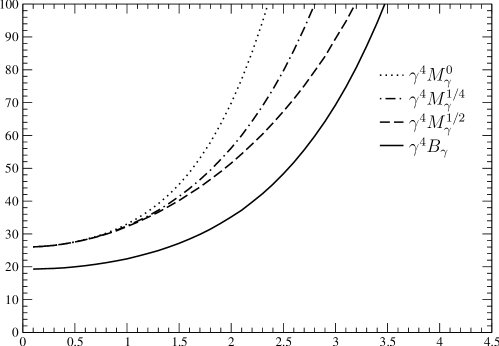
Figure 1: $\gamma^{4}B_{\gamma}$ and $\gamma^{4}M_{\gamma}^{\alpha}$ ($\gamma\to 0$ asymptotics)

In Figure 2 we illustrate the $\gamma\to\infty$ asymptotics of the limiting mean squared errors by plotting the functions $B_{\gamma}$ and $M_{\gamma}^{\alpha}$ themselves. Here the advantage of the choice $\alpha=1/2$ is obvious, and one can observe that for $\gamma>5$ this choice makes negligible the loss of efficiency resulting from the use of the maximum likelihood estimator instead of the asymptotically efficient Bayesian estimators.

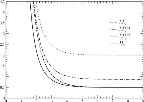
Figure 2: $B_{\gamma}$ and $M_{\gamma}^{\alpha}$ ($\gamma\to\infty$ asymptotics)

Finally, in Figure 3 we illustrate the behavior both at $0$ and at $\infty$ of the asymptotic relative efficiency of the maximum likelihood estimators by plotting the functions $E_{\gamma}^{\alpha}$. All the observations made above can be once more noticed in this figure. Note also that as $\gamma$ increases from $0$ to $\infty$, the asymptotic relative efficiency seems first to decrease from $E_{0}\approx 0.7397$ for all the maximum likelihood estimators, before increasing back to $E_{\infty}^{\alpha}$ for the maximum likelihood estimators with $\alpha$ close to the optimal value $1/2$.

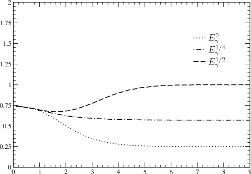
Figure 3: $E_{\gamma}^{\alpha}$ (both asymptotics)

3 Proofs of the lemmas

For the sake of clarity, for each lemma we will first give the proof in the particular Gaussian case (in which it is more explicit) and then explain how it can be extended to the general one.

Proof of Lemma 2

Note that the restrictions of the process $\ln X_{\gamma}(y)=\ln Z_{\gamma}(y/\gamma^{2})$, $y\in\mathbb{R}$, (as well as those of the process $\ln Z_{0}$) on $\mathbb{R}_{+}$ and on $\mathbb{R}_{-}$ are mutually independent processes with stationary and independent increments. So, to obtain the convergence of all the finite-dimensional distributions, it is sufficient to show the convergence of one-dimensional distributions only, that is, the weak convergence of $\ln X_{\gamma}(y)$ to

$$\ln Z_{0}(y)=W(y)-\frac{\left|y\right|}{2}\sim\mathcal{N}\biggl{(}-\frac{\left|y\right|}{2},\left|y\right|\biggr{)}$$

for all $y\in\mathbb{R}$. Moreover, these processes being symmetric, it is sufficient to consider $y\in\mathbb{R}_{+}$ only.

The characteristic function $\varphi_{\gamma}(t)$ of $\ln X_{\gamma}(y)$ is

$$\varphi_{\gamma}(t) =\mathbf{E}\,e^{it\ln X_{\gamma}(y)}=\mathbf{E}\,e^{-it\gamma\sum_{k=1}^{\Pi_{+}\bigl{(}y/\gamma^{2}\bigr{)}}\varepsilon_{k}^{+}-it\frac{\gamma^{2}}{2}\Pi_{+}(y/\gamma^{2})}$$

$$=\mathbf{E}\,\mathbf{E}\,\Bigl{(}e^{-it\gamma\sum_{k=1}^{\Pi_{+}\bigl{(}y/\gamma^{2}\bigr{)}}\varepsilon_{k}^{+}-it\frac{\gamma^{2}}{2}\Pi_{+}(y/\gamma^{2})}\Bigm{|}\mathscr{F}_{\Pi_{+}}\Bigr{)}$$

$$=\mathbf{E}\biggl{(}e^{-it\frac{\gamma^{2}}{2}\Pi_{+}(y/\gamma^{2})}\prod_{k=1}^{\Pi_{+}(y/\gamma^{2})}\mathbf{E}\,e^{-it\gamma\varepsilon_{k}^{+}}\biggr{)}$$

$$=\mathbf{E}\,e^{-it\frac{\gamma^{2}}{2}\Pi_{+}(y/\gamma^{2})-\frac{t^{2}\gamma^{2}}{2}\Pi_{+}(y/\gamma^{2})}=\mathbf{E}\,e^{-\frac{\gamma^{2}}{2}(it+t^{2})\Pi_{+}(y/\gamma^{2})}$$

where we have denoted $\mathscr{F}_{\Pi_{+}}$ the $\sigma$-algebra related to the Poisson process $\Pi_{+}$, used the independence of $\varepsilon_{k}^{+}$ and $\Pi_{+}$ and recalled that $\mathbf{E}\,e^{it\varepsilon}=e^{-t^{2}/2}$.

Then, noting that $\Pi_{+}(y/\gamma^{2})$ is a Poisson random variable of parameter $y/\gamma^{2}$ with moment generating function $\mathbf{E}\,e^{t\Pi_{+}(y/\gamma^{2})}=\exp\bigl{(}\frac{y}{\gamma^{2}}(e^{t}-1)\bigr{)}$, we get

$$\ln\varphi_{\gamma}(t) =\frac{y}{\gamma^{2}}\Bigl{(}e^{-\frac{\gamma^{2}}{2}(it+t^{2})}-1\Bigr{)}=\frac{y}{\gamma^{2}}\Bigl{(}-\frac{\gamma^{2}}{2}(it+t^{2})+o(\gamma^{2})\Bigr{)}$$

$$=-\frac{y}{2}(it+t^{2})+o(1)\to-\frac{y}{2}(it+t^{2})=\ln\mathbf{E}\,e^{it\ln Z_{0}(y)}$$

as $\gamma\to 0$ and so, in the Gaussian case Lemma 2 is proved.

In the general case, proceeding similarly we get

$$\varphi_{\gamma}(t) =\mathbf{E}\,e^{it\ln X_{\gamma,f}(y)}=\mathbf{E}\,e^{it\sum_{k=1}^{\Pi_{+}\bigl{(}y/I\gamma^{2}\bigr{)}}\ln\frac{f(\varepsilon_{k}^{+}+\gamma)}{f(\varepsilon_{k}^{+})}}$$

$$=\mathbf{E}\biggl{(}\Bigl{(}\mathbf{E}\,e^{it\ln\frac{f(\varepsilon+\gamma)}{f(\varepsilon)}}\Bigr{)}^{\Pi_{+}(y/I\gamma^{2})}\biggr{)}\to e^{i\bigl{(}-\frac{y}{2}\bigr{)}t-\frac{1}{2}yt^{2}}=\mathbf{E}\,e^{it\ln Z_{0}(y)}$$

by dominated convergence theorem, since

$$\Bigl{(}\mathbf{E}\,e^{it\ln\frac{f(\varepsilon+\gamma)}{f(\varepsilon)}}\Bigr{)}^{1/\gamma^{2}}\to e^{i\bigl{(}-\frac{I}{2}\bigr{)}t-\frac{1}{2}It^{2}}$$

by (5), and $\gamma^{2}\,\Pi_{+}(y/I\gamma^{2})$ converges clearly to $y/I$ in $L^{2}$ (and hence in probability).

Proof of Lemma 4

Now we turn to the proof of Lemma 4 (we will prove Lemma 3 just after). For $y>0$ we have

$$\mathbf{E}X_{\gamma}^{1/2}(y) =\mathbf{E}\,\mathbf{E}\,\Bigl{(}e^{-\frac{\gamma}{2}\sum_{k=1}^{\Pi_{+}\bigl{(}y/\gamma^{2}\bigr{)}}\varepsilon_{k}^{+}-\frac{\gamma^{2}}{4}\Pi_{+}(y/\gamma^{2})}\Bigm{|}\mathscr{F}_{\Pi_{+}}\Bigr{)}$$

$$=\mathbf{E}\,e^{-\frac{\gamma^{2}}{4}\Pi_{+}(y/\gamma^{2})+\frac{\gamma^{2}}{8}\Pi_{+}(y/\gamma^{2})}=\mathbf{E}\,e^{-\frac{\gamma^{2}}{8}\Pi_{+}(y/\gamma^{2})}$$

$$=\exp\biggl{(}\frac{y}{\gamma^{2}}\Bigl{(}e^{-\frac{\gamma^{2}}{8}}-1\Bigr{)}\biggr{)}.$$

The process $X_{\gamma}$ being symmetric, we have

$$\mathbf{E}X_{\gamma}^{1/2}(y)=\exp\biggl{(}\frac{\left|y\right|}{\gamma^{2}}\Bigl{(}e^{-\frac{\gamma^{2}}{8}}-1\Bigr{)}\biggr{)}$$ (8)

for all $y\in\mathbb{R}$ and, since

$$\frac{1}{\gamma^{2}}\Bigl{(}e^{-\frac{\gamma^{2}}{8}}-1\Bigr{)}=\frac{1}{\gamma^{2}}\Bigl{(}-\frac{\gamma^{2}}{8}+o(\gamma^{2})\Bigr{)}\to-\frac{1}{8}$$

as $\gamma\to 0$, for any $c\in\left]\,0\,{,}\;1/8\,\right[$ we have $\mathbf{E}X_{\gamma}^{1/2}(y)\leqslant\exp\bigl{(}-c\left|y\right|\bigr{)}$ for all sufficiently small $\gamma$ and all $y\in\mathbb{R}$. So, in the Gaussian case Lemma 4 is proved.

In the general case, equality (8) becomes $\mathbf{E}X_{\gamma,f}^{1/2}(y)=\exp\bigl{(}\left|y\right|(I_{\gamma}-1)/I\gamma^{2}\bigr{)}$ with

$$I_{\gamma}=\mathbf{E}\sqrt{\frac{f(\varepsilon+\gamma)}{f(\varepsilon)}}\leqslant\sqrt{\mathbf{E}\,\frac{f(\varepsilon+\gamma)}{f(\varepsilon)}}=1.$$

Recall the convergence (5) of characteristic functions and note that $I_{\gamma}^{1/\gamma^{2}}$ are the corresponding moment generating functions at point $1/2$. The convergence of these moment generating functions (at any point smaller than $1$) follows from the fact that for all $\gamma$ they are equal $1$ at point $1$ (which provides uniform integrability). Thus we have $I_{\gamma}^{1/\gamma^{2}}\to e^{-I/8}$, which implies $(\ln I_{\gamma})/\gamma^{2}\to-I/8$, and so $(I_{\gamma}-1)/I\gamma^{2}\to-1/8$.

Proof of Lemma 3

First we consider the case $y_{1},y_{2}\in\mathbb{R}_{+}$ (say $y_{1}\geqslant y_{2}$). Using (8) and taking into account the stationarity and the independence of the increments of the process $\ln X_{\gamma}$ on $\mathbb{R}_{+}$, we can write

$$\mathbf{E}\left|X_{\gamma}^{1/2}(y_{1})-X_{\gamma}^{1/2}(y_{2})\right|^{2} =\mathbf{E}X_{\gamma}(y_{1})+\mathbf{E}X_{\gamma}(y_{2})-2\,\mathbf{E}X_{\gamma}^{1/2}(y_{1})X_{\gamma}^{1/2}(y_{2})$$

$$=2-2\,\mathbf{E}X_{\gamma}(y_{2})\,\mathbf{E}\,\frac{X_{\gamma}^{1/2}(y_{1})}{X_{\gamma}^{1/2}(y_{2})}$$

$$=2-2\,\mathbf{E}X_{\gamma}^{1/2}\bigl{(}\left|y_{1}-y_{2}\right|\bigr{)}$$

$$=2-2\exp\biggl{(}\frac{\left|y_{1}-y_{2}\right|}{\gamma^{2}}\Bigl{(}e^{-\frac{\gamma^{2}}{8}}-1\Bigr{)}\biggr{)}$$

$$\leqslant-2\,\frac{\left|y_{1}-y_{2}\right|}{\gamma^{2}}\Bigl{(}e^{-\frac{\gamma^{2}}{8}}-1\Bigr{)}\leqslant\frac{1}{4}\left|y_{1}-y_{2}\right|.$$

The process $X_{\gamma}$ being symmetric, we have the same result for the case $y_{1},y_{2}\in\mathbb{R}_{-}$.

Finally, if $y_{1}y_{2}\leqslant 0$ (say $y_{2}\leqslant 0\leqslant y_{1}$), we have

$$\mathbf{E}\left|X_{\gamma}^{1/2}(y_{1})-X_{\gamma}^{1/2}(y_{2})\right|^{2} =2-2\,\mathbf{E}X_{\gamma}^{1/2}(y_{1})\,\mathbf{E}X_{\gamma}^{1/2}(y_{2})$$

$$=2-2\exp\biggl{(}\frac{\left|y_{1}\right|}{\gamma^{2}}\Bigl{(}e^{-\frac{\gamma^{2}}{8}}-1\Bigr{)}+\frac{\left|y_{2}\right|}{\gamma^{2}}\Bigl{(}e^{-\frac{\gamma^{2}}{8}}-1\Bigr{)}\biggr{)}$$

$$=2-2\exp\biggl{(}\frac{\left|y_{1}-y_{2}\right|}{\gamma^{2}}\Bigl{(}e^{-\frac{\gamma^{2}}{8}}-1\Bigr{)}\biggr{)}$$

$$\leqslant\frac{1}{4}\left|y_{1}-y_{2}\right|,$$

and so, in the Gaussian case we obtain even more than the assertion of Lemma 3.

In the general case, proceeding similarly we get

$$\mathbf{E}\left|X_{\gamma,f}^{1/2}(y_{1})-X_{\gamma,f}^{1/2}(y_{2})\right|^{2}\leqslant-2\,\frac{\left|y_{1}-y_{2}\right|}{I\gamma^{2}}(I_{\gamma}-1)$$

and, since $-2(I_{\gamma}-1)/I\gamma^{2}\to 1/4$, the proof is concluded.

Proof of Lemma 5

First let $y_{1},y_{2}\in\mathbb{R}_{+}$ (say $y_{1}\geqslant y_{2}$) such that $\Delta=\left|y_{1}-y_{2}\right|<h$. Then, noting that conditionally to $\mathscr{F}_{\Pi_{+}}$ the random variable

$$\ln X_{\gamma}(\Delta)=-\gamma\sum_{k=1}^{\Pi_{+}(\Delta/\gamma^{2})}\varepsilon_{k}^{+}-\frac{\gamma^{2}}{2}\Pi_{+}(\Delta/\gamma^{2})$$

is Gaussian with mean $-\frac{\gamma^{2}}{2}\Pi_{+}(\Delta/\gamma^{2})$ and variance $\gamma^{2}\Pi_{+}(\Delta/\gamma^{2})$, we get

$$\mathbf{P}\Bigl{\{}\bigl{|}\ln X_{\gamma}(y_{1})-\ln X_{\gamma}(y_{2})\bigr{|}>\delta\Bigr{\}} \leqslant\frac{1}{\delta^{2}}\,\mathbf{E}\bigl{|}\ln X_{\gamma}(y_{1})-\ln X_{\gamma}(y_{2})\bigr{|}^{2}$$

$$=\frac{1}{\delta^{2}}\,\mathbf{E}\bigl{|}\ln X_{\gamma}(\Delta)\bigr{|}^{2}$$

$$=\frac{1}{\delta^{2}}\,\mathbf{E}\,\mathbf{E}\,\Bigl{(}\bigl{(}\ln X_{\gamma}(\Delta)\bigr{)}^{2}\Bigm{|}\mathscr{F}_{\Pi_{+}}\Bigr{)}$$

$$=\frac{1}{\delta^{2}}\,\mathbf{E}\left(\gamma^{2}\Pi_{+}(\Delta/\gamma^{2})+\frac{\gamma^{4}}{4}\bigl{(}\Pi_{+}(\Delta/\gamma^{2})\bigr{)}^{2}\right)$$

$$=\frac{1}{\delta^{2}}\,\Biggl{(}\Delta+\frac{\gamma^{4}}{4}\biggl{(}\frac{\Delta}{\gamma^{2}}+\frac{\Delta^{2}}{\gamma^{4}}\biggr{)}\Biggr{)}$$

$$=\frac{1}{\delta^{2}}\,\bigl{(}(1+\gamma^{2}/4)\Delta+\Delta^{2}/4\bigr{)}$$

$$<\frac{1}{\delta^{2}}\,\bigl{(}\beta(\gamma)\,h+h^{2}/4\bigr{)}$$

where $\beta(\gamma)=1+\gamma^{2}/4\to 1$ as $\gamma\to 0$. So, we have

$$\lim_{\gamma\to 0}\ \sup_{\left|y_{1}-y_{2}\right|<h}\mathbf{P}\Bigl{\{}\bigl{|}\ln X_{\gamma}(y_{1})-\ln X_{\gamma}(y_{2})\bigr{|}>\delta\Bigr{\}} \leqslant\lim_{\gamma\to 0}\frac{1}{\delta^{2}}\,\bigl{(}\beta(\gamma)\,h+h^{2}/4\bigr{)}$$

$$=\frac{1}{\delta^{2}}\left(h+\frac{h^{2}}{4}\right),$$

and hence

$$\lim_{h\to 0}\ \lim_{\gamma\to 0}\ \sup_{\left|y_{1}-y_{2}\right|<h}\mathbf{P}\Bigl{\{}\bigl{|}\ln X_{\gamma}(y_{1})-\ln X_{\gamma}(y_{2})\bigr{|}>\delta\Bigr{\}}=0,$$

where the supremum is taken only over $y_{1},y_{2}\in\mathbb{R}_{+}$.

The process $X_{\gamma}$ being symmetric, we have the same conclusion with the supremum taken over $y_{1},y_{2}\in\mathbb{R}_{-}$.

Finally, for $y_{1}y_{2}\leqslant 0$ (say $y_{2}\leqslant 0\leqslant y_{1}$) such that $\left|y_{1}-y_{2}\right|<h$, using the elementary inequality $(a-b)^{2}\leqslant 2(a^{2}+b^{2})$ we get

$$\mathbf{P}\Bigl{\{}\bigl{|}\ln X_{\gamma}(y_{1})-\ln X_{\gamma}(y_{2})\bigr{|}>\delta\Bigr{\}} \leqslant\frac{1}{\delta^{2}}\,\mathbf{E}\bigl{|}\ln X_{\gamma}(y_{1})-\ln X_{\gamma}(y_{2})\bigr{|}^{2}$$

$$\leqslant\frac{2}{\delta^{2}}\biggl{(}\mathbf{E}\bigl{|}\ln X_{\gamma}(y_{1})\bigr{|}^{2}+\mathbf{E}\Bigl{|}\ln X_{\gamma}\bigl{(}\left|y_{2}\right|\bigr{)}\Bigr{|}^{2}\biggr{)}$$

$$=\frac{2}{\delta^{2}}\bigl{(}\beta(\gamma)y_{1}+y_{1}^{2}/4+\beta(\gamma)\left|y_{2}\right|+\left|y_{2}\right|^{2}/4\bigr{)}$$

$$<\frac{2}{\delta^{2}}\Bigl{(}\beta(\gamma)h+h^{2}/4\Bigr{)},$$

which again yields the desired conclusion. So, in the Gaussian case Lemma 5 is proved.

Another way to prove this lemma, is to notice first that the weak convergence of $\ln X_{\gamma}(y)$ to $\ln Z_{0}(y)$ (established in Lemma 2) is uniform with respect to $y\in K$ for any compact $K\subset\mathbb{R}$. Indeed, the uniformity of the convergence of the characteristic functions in the proof of Lemma 2 is obvious, and so one can apply, for example, Theorem 7 from Appendix I of [15], whose remaining conditions are easily checked.

Second, using this uniformity we obtain

$$\lim_{\gamma\to 0}\ \sup_{\left|y_{1}-y_{2}\right|<h}\mathbf{P}\Bigl{\{}\bigl{|}\ln X_{\gamma}(y_{1})-\ln X_{\gamma}(y_{2})\bigr{|}>\delta\Bigr{\}} =\lim_{\gamma\to 0}\ \sup_{\left|y\right|<h}\mathbf{P}\Bigl{\{}\bigl{|}\ln X_{\gamma}(y)\bigr{|}>\delta\Bigr{\}}$$

$$=\sup_{\left|y\right|<h}\mathbf{P}\Bigl{\{}\bigl{|}\ln Z_{0}(y)\bigr{|}>\delta\Bigr{\}}$$

where the supremum is taken over $y_{1},y_{2}\in\mathbb{R}$ such that $y_{1}y_{2}\geqslant 0$, and

$$\lim_{\gamma\to 0}\ \sup_{\left|y_{1}-y_{2}\right|<h}\mathbf{P}\Bigl{\{}\bigl{|}\ln X_{\gamma}(y_{1})-\ln X_{\gamma}(y_{2})\bigr{|}>\delta\Bigr{\}}\leqslant 2\sup_{\left|y\right|<h}\mathbf{P}\Bigl{\{}\bigl{|}\ln Z_{0}(y)\bigr{|}>\frac{\delta}{2}\Bigr{\}}$$

where the supremum is taken over $y_{1},y_{2}\in\mathbb{R}$ such that $y_{1}y_{2}\leqslant 0$.

Finally, reminding that $\ln Z_{0}(y)\sim\mathcal{N}\bigl{(}-\left|y\right|/2\,,\,\left|y\right|\bigr{)}$ and denoting $\Phi$ the distribution function of the standard Gaussian law, we get

$$\mathbf{P}\Bigl{\{}\bigl{|}\ln Z_{0}(y)\bigr{|}>\delta\Bigr{\}} =\Phi\biggl{(}-\frac{\delta}{\sqrt{\left|y\right|}}+\frac{\sqrt{\left|y\right|}}{2}\,\biggr{)}+1-\Phi\biggl{(}\frac{\delta}{\sqrt{\left|y\right|}}+\frac{\sqrt{\left|y\right|}}{2}\,\biggr{)}$$

$$\leqslant\Phi\biggl{(}-\frac{\delta}{\sqrt{h}}+\frac{\sqrt{h}}{2}\,\biggr{)}+1-\Phi\biggl{(}\frac{\delta}{\sqrt{h}}\biggr{)}$$

for $\left|y\right|<h$. The last expression does not depend on $y$ and clearly converges to $0$ as $h\to 0$, so the assertion of the lemma follows.

It remains to observe that this second proof does not use any particularity of the process $X_{\gamma}$ and, hence, is trivially extendable to the general case.

Proof of Lemma 6

Taking into account the symmetry of the process $\ln X_{\gamma}$, as well as the stationarity and the independence of its increments on $\mathbb{R}_{+}$, we obtain

$$\mathbf{P}\biggl{\{}\sup_{\left|y\right|>A}X_{\gamma}(y)>e^{-bA}\biggr{\}} \leqslant 2\,\mathbf{P}\biggl{\{}\sup_{y>A}X_{\gamma}(y)>e^{-bA}\biggr{\}}$$ (9)

$$\leqslant 2\,e^{\,bA/2}\;\mathbf{E}\sup_{y>A}X_{\gamma}^{1/2}(y)$$

$$=2\,e^{\,bA/2}\;\mathbf{E}X_{\gamma}^{1/2}(A)\;\mathbf{E}\sup_{y>A}\frac{X_{\gamma}^{1/2}(y)}{X_{\gamma}^{1/2}(A)}$$

$$=2\,e^{\,bA/2}\;\mathbf{E}X_{\gamma}^{1/2}(A)\;\mathbf{E}\sup_{z>0}X_{\gamma}^{1/2}(z).$$

In order to estimate the last factor we write

$$\mathbf{E}\sup_{z>0}X_{\gamma}^{1/2}(z) =\mathbf{E}\exp\left(\frac{1}{2}\,\sup_{z>0}\,\Biggl{(}-\gamma\sum_{k=1}^{\Pi_{+}(z/\gamma^{2})}\varepsilon_{k}^{+}-\frac{\gamma^{2}}{2}\Pi_{+}(z/\gamma^{2})\Biggr{)}\right)$$

$$=\mathbf{E}\exp\left(\frac{1}{2}\,\sup_{n\in\mathbb{N}}\,\biggl{(}-\gamma\sum_{k=1}^{n}\varepsilon_{k}^{+}-\frac{n\gamma^{2}}{2}\biggr{)}\right).$$

Now, let us observe that the random walk $S_{n}=-\sum_{k=1}^{n}\varepsilon_{k}^{+}$, $n\in\mathbb{N}$, has the same law as the restriction on $\mathbb{N}$ of a standard Brownian motion $W$. So,

$$\mathbf{E}\sup_{z>0}X_{\gamma}^{1/2}(z) =\mathbf{E}\exp\left(\frac{1}{2}\,\sup_{n\in\mathbb{N}}\,\bigl{(}\gamma W(n)-n\gamma^{2}/2\bigr{)}\right)$$

$$=\mathbf{E}\exp\left(\frac{1}{2}\,\sup_{n\in\mathbb{N}}\,\bigl{(}W(n\gamma^{2})-n\gamma^{2}/2\bigr{)}\right)$$

$$\leqslant\mathbf{E}\exp\left(\frac{1}{2}\,\sup_{t>0}\,\bigl{(}W(t)-t/2\bigr{)}\right)=\mathbf{E}\exp\left(\frac{1}{2}\,M\right)$$

with an evident notation. It is known that the random variable $M$ is exponential of parameter $1$ $\bigl{(}$see, for example, [3]$\bigr{)}$ and hence, using its moment generating function $\mathbf{E}\,e^{tM}=(1-t)^{-1}$, we get

$$\mathbf{E}\sup_{z>0}X_{\gamma}^{1/2}(z)\leqslant 2.$$ (10)

Finally, taking $b\in\left]\,0\,{,}\;1/12\,\right[$ we have $3b/2\in\left]\,0\,{,}\;1/8\,\right[$ and, combining (9), (10) and using Lemma 4, we finally obtain

$$\mathbf{P}\biggl{\{}\sup_{\left|y\right|>A}X_{\gamma}(y)>e^{-bA}\biggr{\}} \leqslant 4\,e^{\,bA/2}\,\exp\Bigl{(}-\frac{3b}{2}A\Bigr{)}=4\,e^{-bA}$$

for all sufficiently small $\gamma$ and all $A>0$, which concludes the proof in the Gaussian case.

In the general case the proof is almost the same. Note that we have no longer the symmetry of the process $X_{\gamma,f}$, so we need to consider the cases $y>A$ and $y<-A$ separately. Besides that, the only difference is in the derivation of the bound (10). Here we get

$$\mathbf{E}\sup_{z>0}X_{\gamma,f}^{1/2}(z)=\mathbf{E}\exp\left(\frac{1}{2}\,M\right),$$

where $M$ is the supremum of the random walk $S_{n}=\sum_{k=1}^{n}X_{k}$, $n\in\mathbb{N}$, with $X_{k}=\ln\frac{f(\varepsilon_{k}^{+}+\gamma)}{f(\varepsilon_{k}^{+})}\,$. Note that

$$\mathbf{E}\,e^{X_{1}}=\mathbf{E}\,\frac{f(\varepsilon+\gamma)}{f(\varepsilon)}=1,$$

and so, the cummulant generating function $k(t)=\ln(\mathbf{E}\,e^{tX_{1}})$ of $X_{1}$ admits a strictly positive zero $t_{0}=1$. Hence, by the well-known Cramér-Lundberg bound on the tail probabilities of $M$ $\bigl{(}$see, for example, Theorem 5.1 from Chapter XIII of [1]$\bigr{)}$, we have

$$\mathbf{P}(M>x)\leqslant e^{-t_{0}\,x}=e^{-x}$$

for all $x>0$. Finally, denoting $F$ the distribution function of $M$ and using this bound we obtain

$$\mathbf{E}\exp\left(\frac{1}{2}\,M\right) =\int_{\mathbb{R}}e^{\,x/2}\;dF(x)$$

$$=\Bigl{[}e^{\,x/2}\bigl{(}F(x)-1\bigr{)}\Bigr{]}_{-\infty}^{+\infty}-\;\frac{1}{2}\int_{\mathbb{R}}e^{\,x/2}\bigl{(}F(x)-1\bigr{)}\;dx$$

$$=\frac{1}{2}\int_{\mathbb{R}_{-}}e^{\,x/2}\;dx+\frac{1}{2}\int_{\mathbb{R}_{+}}e^{\,x/2}\bigl{(}1-F(x)\bigr{)}\;dx$$

$$\leqslant 1+\frac{1}{2}\int_{\mathbb{R}_{+}}e^{-x/2}\;dx=2,$$

which concludes the proof.

References

- [1] Asmussen, S., “Applied probability and queues”, 2nd ed., Applications of Mathematics 51, Springer-Verlag, New York, 2003.
- [2] Bhattacharya, P.K. and Brockwell, P.J., “The minimum of an additive process with applications to signal estimation and storage theory”, Z. Wahrsch. verw. Geb. 37, no. 1, pp. 51–75, 1976.
- [3] Borodin, A.N. and Salminen, P., “Handbook of Brownian motion — facts and formulae”, Probability and its Applications, Birkhäuser Verlag, Basel, 2002.
- [4] Chan, K.S., “Consistency and limiting distribution of the least squares estimator of a threshold autoregressive model”, Ann. Statist. 21, no. 1, pp. 520–533, 1993.
- [5] Chan, N.H. and Kutoyants, Yu.A., “On parameter estimation of threshold autoregressive models”, submitted. http://arxiv.org/abs/1003.3800
- [6] Ciuperca, G., “Maximum likelihood estimator in a two-phase nonlinear random regression model”, Statist. Decisions 22, no. 4, pp. 335–349, 2004.
- [7] Dachian, S., “On limiting likelihood ratio processes of some change-point type statistical models”, J. Statist. Plann. Inference 140, no. 9, pp. 2682–2692, 2010.
- [8] Dachian, S. and Negri I., “On compound Poisson type limiting likelihood ratio process arising in some change-point models”, WP n.11/MS, Dep. IIMM, 2009. http://hdl.handle.net/10446/529
- [9] Dachian, S. and Negri I., “On Gaussian Compound Poisson Type Limiting Likelihood Ratio Process”, Proceedings of the 45th Scientific Meeting of the Italian Statistical Society, 2010. http://homes.stat.unipd.it/mgri/SIS2010/Program/contributedpaper/737-1258-1-DR.pdf
- [10] Fujii, T., “A note on the asymptotic distribution of the maximum likelihood estimator in a non-regular case”, Statist. Probab. Lett. 77, no. 16, pp. 1622–1627, 2007.
- [11] Gihman, I.I. and Skorohod, A.V., “The theory of stochastic processes I”, Springer-Verlag, New York, 1974.
- [12] Golubev, G.K., “Computation of the efficiency of the maximum-likelihood estimator when observing a discontinuous signal in white noise”, Problems Inform. Transmission 15, no. 3, pp. 61–69, 1979.
- [13] Höpfner, R. and Kutoyants, Yu.A., “Estimating discontinuous periodic signals in a time inhomogeneous diffusion”, submitted. http://arxiv.org/abs/0903.5061
- [14] Ibragimov, I.A. and Khasminskii, R.Z., “Estimation of a parameter of a discontinuous signal in a white Gaussian noise”, Problems Inform. Transmission 11, no. 3, pp. 31–43, 1975.
- [15] Ibragimov, I.A. and Khasminskii, R.Z., “Statistical estimation. Asymptotic theory”, Springer-Verlag, New York, 1981.
- [16] Koul, H.L. and Qian, L., “Asymptotics of maximum likelihood estimator in a two-phase linear regression model”, J. Statist. Plann. Inference 108, no. 1–2, pp. 99–119, 2002.
- [17] Küchler, U. and Kutoyants, Yu.A., “Delay estimation for some stationary diffusion-type processes”, Scand. J. Statist. 27, no. 3, pp. 405–414, 2000.
- [18] Kutoyants, Yu.A., “Parameter estimation for stochastic processes”, Armenian Academy of Sciences, Yerevan, 1980 (in Russian), translation of revised version, Heldermann-Verlag, Berlin, 1984.
- [19] Kutoyants, Yu.A., “Identification of dynamical systems with small noise”, Mathematics and its Applications 300, Kluwer Academic Publishers Group, Dordrecht, 1994.
- [20] Kutoyants, Yu.A., “Statistical inference for ergodic diffusion processes”, Springer Series in Statistics, Springer-Verlag, London, 2004.
- [21] Rubin, H. and Song, K.-S., “Exact computation of the asymptotic efficiency of maximum likelihood estimators of a discontinuous signal in a Gaussian white noise”, Ann. Statist. 23, no. 3, pp. 732–739, 1995.
- [22] Terent’yev, A.S., “Probability distribution of a time location of an absolute maximum at the output of a synchronized filter”, Radioengineering and Electronics 13, no. 4, pp. 652–657, 1968.
- [23] Yao, Y.-C., “Approximating the distribution of the maximum likelihood estimate of the change-point in a sequence of independent random variables”, Ann. Statist. 15, no. 3, pp. 1321–1328, 1987.