Cache Me If You Can: Capacitated Selfish Replication Games in Networks

Abstract

In Peer-to-Peer (P2P) network systems, content (object) delivery between nodes is often required. One way to study such a distributed system is by defining games, which involve selfish nodes that make strategic choices on replicating content in their local limited memory (cache) or accessing content from other nodes for a cost. These Selfish Replication games have been introduced in Chun et al (2004) for nodes that do not have any capacity limits, leaving the capacitated problem, i.e. Capacitated Selfish Replication (CSR) games, open.

In this work, we first form the model of the CSR games, for which we perform a Nash equilibria analysis. In particular, we focus on hierarchical networks, given their extensive use to model communication costs of content delivery in P2P systems. We present an exact polynomial-time algorithm for any hierarchical network, under two constraints on the utility functions: 1) “Nearer is better”, i.e. the closest the content is to the node the less its access cost is, and 2) “Independence of irrelevant alternatives”, i.e. aggregation of individual node preferences. This generalization represents a vast class of utilities and more interestingly allows each of the nodes to have simultaneously completely different functional forms of utility functions. In this general framework, we present CSR games results on arbitrary networks and outline the boundary between intractability and effective computability in terms of the network structure, object preferences, and the total number of objects. Moreover, we prove that the problem of equilibria existence becomes NP-hard for general CSR games. By adding some constraints in the number of objects and their preferences, we show that the equilibrium can be found in polynomial time. Finally, we introduce the fractional version of CSR games (F-CSR) to represent content distribution. We prove that equilibrium exists for every F-CSR game, but it is PPAD-complete.

1 Introduction

Consider a P2P network for sharing movies (objects) among multiple users (nodes). Due to limited disk space, the movies can be stored either locally or obtained from other users in some cost. The storing decisions affect everyone that uses this service. A natural question is to predict the movie collection stability in your friends network (i.e. equilibrium) and your satisfaction from them (i.e. access cost), when users act selfishly. Similarly, in the new wireless 4G services, users will not only consume different apps, but will also provide apps to their network through personal communications and computing devices. In such a network, the question is whether storing apps will lead to a situation of endless churn or could there be an equilibrium?

Content delivery and caching in P2P networks can be studied in a game-theoretic framework. In this work, we study Capacitated Selfish Replication (CSR) games as an abstraction of the above network scenarios. In CSR games the strategic agents, or players, are nodes in a network that act selfishly. The nodes have some object preferences and bounded storage space, i.e. caches, to store a limited number of content copies. Each node in cooperation with other nodes can serve access requests for the objects that are stored in its cache. However, the set of objects which a node chooses to store in its cache is from one side solely based on its own utility function (notice that this does not prevent the players to use the same utility function for the whole network) and from the other side based on where objects of interest have been stored in the network. Thus, each node in the model, has two potential actions for an object. Either store a replica of the object in its limited cache, or access with some cost the object replica from a remote node.

Chun et al. Chun et al (2004) first introduced such a game-theoretic framework to analyse pure Nash equilibria in networks without cache capacities, but with some storage cost. They left the capacitated version of the problem open. The main interest of the CSR games in more recent works is on hierarchical networks that have been extensively used to model communication content delivery costs in P2P networks Garces-Erice et al (2003). Ultrametric models for content delivery networks Karger et al (1997) and cooperative caching in hierarchical networks Leff et al (1993); Tewari et al (1999); Korupolu et al (2001); Korupolu and Dahlin (2002) are just some examples. The best results on CSR games for hierarchical networks Laoutaris et al (2006b); Pollatos et al (2008) are about the existence of a Nash equilibrium for a generalized one-level hierarchical network, using the sum utility function for which each node is based on a weighted sum of the cost of accessing the objects.

1.1 Our results

In this paper, we first introduce the basic model of the Capacitated Selfish Replication (CSR) games in Section 2. This includes the definition of the nodes (players) and objects, the formulation of the cost functions for a node accessing objects in the network, the object replication strategies among nodes, as well as the basic formulation of the network. The main focus is on the study of Nash equilibria existence and computability for a set of CSR games variants. In particular, we introduce a polynomial-time Nash equilibrium method for hierarchical networks, given their extensive use to model communication costs of content delivery in P2P systems. We address the following three problems, including their computational complexity:

• Does pure Nash equilibrium exist in a CSR game, for hierarchical networks?

• Does pure Nash equilibrium exist in a CSR game, for general undirected networks, setting specific restrictions on the number of objects and the utility/cost functions?

• Does pure Nash equilibrium exist, when the objects can be split in fractions, i.e. F-CSRgames?

Note that in all the games, we assume that all the pieces of content, i.e. objects, have the same size, as considered in prior works Chun et al (2004); Laoutaris et al (2006b); Pollatos et al (2008); Angel et al (2013). Otherwise, the problem becomes NP-hard even for computing the best response of a player (node) as a generalization of the well-known knapsack problem.

In Section 3 we present our main algorithm, which extends and resolves the open problem that was defined in Laoutaris et al (2006a, 2007); Pollatos et al (2008). In particular, it has been proved Laoutaris et al (2006b); Pollatos et al (2008) that CSR games for hierarchical networks have a Nash equilibrium in the case of a generalized $1$-level hierarchy, when the utility function is a function of the costs sum of accessing replicated objects in the network. We introduce an exact polynomial-time algorithm for Nash Equilibrium computation in any hierarchical network. We use a novel technique which we name “fictional players” method. We show that using this method we can extend to a general framework of natural preference orders that are entirely arbitrary, but follow two natural constraints: “Nearer is better”, i.e. the closest the content is to the node the less its access cost is and “Independence of irrelevant alternatives”, i.e. the aggregation of individual node preferences. This generalization represents a vast class of utility functions and more interestingly allows each of the nodes to have simultaneously completely different functional forms of utility functions. The method introduces and iteratively eliminates fictional players in a controlled fashion, maintaining a Nash equilibrium at each step. In the end, the desired equilibrium for the entire network is realized without any fictional players left in the network. Even though the analysis is specified in the context of the sum utility function to elucidate the technique of fictional players, we then abstract the central requirements for our proof technique. In particular, we develop a general framework of CSRgames with ordinal preferences, for which a larger class of utility functions could be used as extension to the above result.

In Section 4, we present the general CSR games framework in terms of the utility preference relations and node preference orders. In particular, we consider the utility that is not just each node’s specific numeric assignment for each objects placement, but a preference order each node has on object placements that satisfies two natural constraints: Monotonicity (or “Nearer is better”) and Consistency (or “Independence of irrelevant alternatives”). In this way the method is extended to a vast class of utility functions, while nodes may simultaneously have utility functions of completely different functional forms.

After extending our hierarchical networks results to the broader class of utilities, in Sections 5 and 6 we study general CSR games that have various network structures (directed or undirected), forms of object preferences (binary or general). Intractability and effective computability of equilibria is delineated in terms of the network structure, object preferences, and the total number of objects. The results are summarized in Table 1. Most notable are the following results:

• equilibria existence for general undirected networks with two objects, using the technique of fictional players

• equilibria existence for general undirected networks when object preferences are binary

• the problem of equilibria existence becomes NP-hard for general CSR games

• equivalence of finding equilibria in polynomial time for CSR games in strongly connected networks with two objects and binary object preferences, via a reduction to the well-studied even-cycle problem Robertson et al (1999).

Object preferences and count	Undirected networks	Directed networks
Binary, two objects	Yes, in P (5.3)	No, in P  (6.2)
Binary, three or more objects	Yes, in PLS (5.2)	No, NP-complete (6.1)
General, two objects	Yes, in P (5.3)	No, NP-complete (6.1)
General, three or more objects	No, NP-complete (6.1)	No, NP-complete (6.1)
	Hierarchical: Yes, in P (5.1)

Table 1: Equilibria existence and computability in CSR games. Each cell (other than in the first row/column) first indicates whether equilibria always exist for a particular CSR games sub-class. If so, the cell next indicates the complexity of determining an equilibrium; otherwise, it indicates the complexity of determining whether equilibria exist. The relevant subsection appears in parentheses.

Finally in Section 7, we introduce the fractional version of CSR games (F-CSR) to represent content distribution using erasure codes. In this framework, each node is allowed to store fractions of objects and can satisfy an object access request by retrieving any set of object fractions as long as these fractions sum to at least one. We present a natural implementation of this framework via erasure codes (e.g. using the Digital Fountain approach Byers et al (1998); Shokrollahi (2006)). We prove that F-CSR games always have equilibria and finding it is in PPAD. However, we also show finding equilibria is PPAD-hard even for a sum-of-distances utility function.

1.2 Related work

Peer-to-Peer (P2P) networks have been used to model systems for sharing content and resources among the individual peers (such as the file systems Kubiatowicz et al (2000); Dabek et al (2001); Rowstron and Druschel (2001); Saito et al (2002), web caches Danzig (1998); Fan et al (1998), or P2P caches Iyer et al (2002)). Even though P2P networks have been extensively studied from a theoretical point of view, there are several open problems when rational peers have diverse and selfish interests Feldman and Chuang (????).

One of the most interesting problems is caching, i.e. holding copies of content in clients and servers. Several research studies have considered data storing Gribble et al (2001); Chen et al (2002), self-stabilization Ko and Rubenstein (2005), dynamic replication Rabinovich et al (1999); Douceur and Wattenhofer (2001); Tang and Chanson (2002), and exchanging of content copies in a centralized manner Li et al (1999); Jamin et al (2000); Qiu et al (2001); Jamin et al (2001). Research on capacitated caching has been also considerable as an optimization problem and various centralized and distributed algorithms have been presented for different networks in Leff et al (1993); Wolfson et al (1997); Korupolu et al (2001); Baev et al (2008); Angel et al (2013). For instance, centralized optimization for the facility location problem has been studied in Rosenwein (1994), including several approximations Jain and Vazirani (1999); Mettu and Plaxton (2000); Mahdian et al (2002). These frameworks usually ignore the fact that peers may make free choices that minimizes their content access cost, by not following usual instrumentation.

The caching problem that we study is in the intersection of game theory and computer science, that has been extensively studied the last decade Nisan et al (2007); Tsaknakis et al (2008). In Papadimitriou (1994) Papadimitriou laid the groundwork for algorithmic game theory by introducing syntactically defined sub-classes of FNP with complete problems, PPAD being a notable such subclass. Non-cooperative facility location games have attracted some small attention over the last decades. For instance, in Vetta (2002), the problem of Nash equilibrium for games that allowed players build nodes in remote locations, whereas in our case nodes hold fixed spaces for storing objects/content. In Goemans et al (2006a), content distribution was studied, providing bounds on the approximated Nash equilibrium with respect to the price of anarchy and the convergence speed. The difference in the game design lies in the fact that each node had cost limits for storing objects without considering network latencies. The uncapacitated case of selfish caching games was introduced in Chun et al (2004), in which nodes could store more pieces of content by paying for the additional storage.

We focus on the capacitated version which was left open by Chun et al (2004), believing that limits on cache-capacity model an important real-world restriction. Special cases of the integral CSR games version have been studied. In Laoutaris et al (2006b), Nash equilibria were shown to exist in cases that nodes are equidistant from one another and a special centralized server holds all objects. In Pollatos et al (2008) the model is slightly extended to the case where special servers for different objects are at different distances. Our results generalize and completely subsume all these prior cases of CSR games. Market sharing games Goemans et al (2006b) also consider caches with capacity, but differ to cc games since they are special cases of congestion games. In this work we focus primarily on equilibria and our general framework of CSRgames with ordinal preferences aligns more with the theory of social choice Arrow (1951); in this sense, we deviate from prior work Fabrikant et al (2003); Devanur et al (2005) that is focused on the price of anarchy Koutsoupias and Papadimitriou (1999).

Our work on CSR games in Gopalakrishnan et al (2012) has initiated various research lines and has been extended recently in different directions. For instance, in Hu and Gong (2013, 2014) the selfish replication problem is studied for the case that nodes seek object placements with cache cooperation, and includes an experimental analysis. Etesami et al. have extended our model in a series of papers Etesami and Başar (2017). In Etesami and Basar (2014) the Nash equilibrium algorithm for two resources is shown to converge faster and it is extended to arbitrary cache sizes for a polynomial time computation. This is extended in Etesami and Başar (2015); Etesami and Basar (2016a, b), where a quasi-polynomial algorithm is introduced to drive allocations whose total cost is within a constant factor of that in any pure-strategy Nash equilibrium, in games formed by undirected networks. The price of anarchy for CSR games with binary preferences over general undirected networks has been studied in Etesami and Basar (2016c); Etesami and Başar (2017), showing an upper bound of $3$. In Pacifici (2016), the caching problem is studied for operator-specific, non-linear, cost functions in games that form arbitrary peering graph topologies, while in Ahmadyan et al (2016) CSR games are studied for general undirected networks for which a randomized algorithm is introduced using a random tree search method to search for pure-strategy Nash equilibrium.

In related work, through a major breakthrough Daskalakis et al (2006); Chen et al (2009) it has been proven that 2-player Nash Equilibrium is PPAD-complete. The PPAD-complete term is coming to occupy a role in algorithmic game theory analogous to NP-completeness in combinatorial optimization Garey and Johnson (1979), and thus we study the fractional version of the problem, where nodes can store parts of objects, while accessing the remaining part from other nodes. In this setup we prove PPAD-completeness.

2 A basic model for CSR games

We consider a set $V$ of nodes (labeled $1$ through $n=|V|$) to form a network in which they share a collection O of unit-size objects. We let $d_{ij}$ denote $i$’s cost for accessing an object at $j$, for $i,j\in V$; we refer to $d$ as the access cost function. $j$ is node’s $i$ nearest node in a set $S$ of nodes, if $j\in S$ and $d_{ij}\leq d_{ik}$ for all $k\in S$. Moreover, a given network is undirected if $d$ is symmetric, i.e. if $d_{ij}=d_{ji}$ for all $i,j\in V$. An undirected network is hierarchical if the access cost function forms an ultrametric, i.e. if $d_{ik}\leq\max\{d_{ij},d_{jk}\}$ for all $i,j,k\in V$.

The cache of each node $i$ is able to store a certain number of objects. Node’s $i$ placement is simply the set of objects stored at $i$. The strategy set of a given node is the set of all feasible placements at the node. A global placement is any tuple $(P_{i}:i\in V)$, where $P_{i}\subseteq\mbox{{\cal O}}$ represents a feasible placement at node $i$. We are going to use $P_{-i}$ to denote the collection $(P_{j}:j\in V\setminus\{i\})$, for convenience. We will also often use $P=(P_{i},P_{-i})$ to refer to a global placement. Moreover, we also assume that $V$ includes a server node that has the capacity to store all the objects. In this way it is ensured that at least one copy of every object is present in the system; this assumption is without loss of generality given that the access cost of every node to the server can be set an arbitrarily large number.

CSR Games. Each node in our game-theoretic model, attaches a utility to each global placement. We assume that each node $i$ has a weight $r_{i}(\alpha)$ for each object $\alpha$ representing the rate at which $i$ accesses $\alpha$. We define the sum utility function $U_{s}(i)$ as follows: $U_{s}(i)(P)=-\sum_{\alpha\in\mbox{{\cal O}}}r_{i}(\alpha)\cdot d_{i\sigma_{i}(P,\alpha)}$, where $\sigma_{i}(P,\alpha)$ is $i$’s nearest node holding $\alpha$ in $P$. A CSR game is a tuple $(V,\mbox{{\cal O}},d,\{r_{i}\})$. This work focuses on pure Nash equilibria (henceforth, simply equilibria) of the CSR games. Such a CSR game equilibrium instance is a global placement $P$ such that for each $i\in V$ there is no placement $Q_{i}$ such that $U_{s}(i)(P)<U_{s}(i)(Q)$.

Unit cache capacity. In this work, we assume that all objects are of identical size. Under this assumption, we now argue that it is sufficient to consider the case where each node’s cache holds exactly one object. Consider a set $V$ of nodes in which the cache of node $i$ can store $c_{i}$ objects. Let $V^{\prime}$ denote a new set of nodes which contains, for each node $i$ in $V$, new nodes $i_{1},i_{2},\ldots,i_{c_{i}}$, i.e., one new node for each unit of the cache capacity of $i$. We extend the access cost function as follows: $d_{j_{\ell}i_{k}}=d_{ji}$ for all $1\leq\ell\leq c_{j}$, $1\leq k\leq c_{i}$ and $d_{i_{\ell}i_{k}}=0$ for all $1\leq\ell<k\leq c_{i}$, for each node $i\in V$.

We consider an obvious onto mapping $f$ from placements in $V^{\prime}$ to those in $V$. Given placement $P^{\prime}$ for $V^{\prime}$, we set $f(P^{\prime})=P$ where $P_{i}=\cup_{1\leq k\leq c_{i}}P^{\prime}_{i_{k}}$. This mapping ensures that $U_{s}(i)(P^{\prime})=U_{s}(i)(P)$, giving us the desired reduction. Thus, in the remainder of the paper, we assume that every node in the network stores at most one object in its cache.

3 Hierarchical networks

In this section, we present a polynomial-time equilibria construction for CSR games on hierarchical networks. We can represent any hierarchical network by a tree $T$ in such a way that the node set $V$ is the set of its leaves. Every internal node $v$ has a label $\ell(v)$ such that:

1. if $v$ is an ancestor of $w$ in $T$, then $\ell(v)\geq\ell(w)$

2. for any $i,j\in V$, $d_{ij}$ is given by $\ell(\mbox{lca}(i,j))$, where $\mbox{lca}(i,j)$ is the least common ancestor of nodes $i$ and $j$ Karger et al (1997); Korupolu et al (2001).

Fig. 1 illustrates a simple example for a hierarchical network tree with two internal nodes and three leaf nodes, with the corresponding label relationships, the least common ancestors, and the access costs.

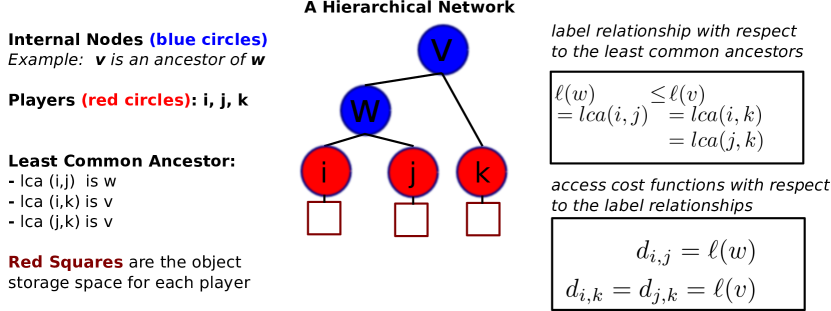
Figure 1: A simple example of a hierarchical network tree with two internal nodes ($\ell(v)$ and $\ell(w)$) and three leaf nodes (i, j, and k). The label relationships, the least common ancestors, and the access costs are described.

Fictional players. The proposed algorithm requires the introduction of the fictional player notion. A fictional $\alpha$-player for an object $\alpha$ will be a new node which stores $\alpha$ in any equilibrium. In particular, for any fictional $\alpha$-player $\ell$, $r_{\ell}(\alpha)$ is $1$ and $r_{\ell}(\beta)$ is $0$ for any $\beta\neq\alpha$. In a particular hierarchy each fictional player is introduced as a leaf; our method determines the exact locations in the hierarchy. The access cost function for each fictional player is naturally extended using the hierarchy and the labels of the internal nodes. We let “node” denote both the elements of $V$ and fictional players.

A preference relation. The object weights for each node $i$ in a hierarchical network induce a natural preorder $\sqsupseteq_{i}$ among elements of $\mbox{{\cal O}}\times A_{i}$, where $A_{i}$ is the set of proper ancestors of $i$ in $T$. In particular, we define $(\alpha,v)\sqsupset_{i}(\beta,w)$ whenever $r_{i}(\alpha)\cdot\ell(v)>r_{i}(\beta)\cdot\ell(w)$. In words, in hierarchical networks there is a total preorder in the objects-nodes preferences, which is used during the algorithm to define a potential function, when nodes are playing their best responses. For instance, $(\alpha,v)\sqsupset_{i}(\beta,w)$ means that if $i$ needs to place either $\alpha$ or $\beta$ in its cache, and the least common ancestor of $i$ and the most $i$-preferred node in $V\setminus\{i\}$ holding $\alpha$ (resp., $\beta$) is $v$ (resp., $w$), then $i$ prefers to store $\alpha$ over $\beta$. Fig. 2 illustrates an example of node $i$ that will prefer to store object $\alpha$ that is stored further than object $\beta$ and with a higher cost, due to the total preorder.

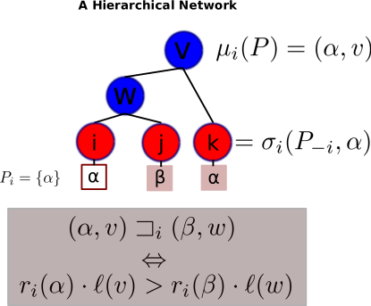
Figure 2: A simple example of a hierarchical network tree with two internal nodes ($\ell(v)$ and $\ell(w)$) and three leaf nodes (i, j, and k). The preference relation of node $i$ is presented.

To express any player’s best response in terms of these preference relations, we define $\mu_{i}(P)=(\alpha,v)$, where $P_{i}=\{\alpha\}$ and $v$ is $\mbox{lca}(i,\sigma_{i}(P_{-i},\alpha))$, where $\sigma_{i}(P_{-i},\alpha)$ denotes $i$’s nearest node in the set of nodes holding $\alpha$ in $P_{-i}$. For instance, in Fig. 2 $\sigma_{i}(P_{-i},\alpha)$ is node $k$ (the nearest node holding $\alpha$), while $P_{i}=\{\alpha\}$ (node $i$ is holding $\alpha$) and the thus, these two information can be denoted as $\mu_{i}(P)=(\alpha,v)$, where $v$ is the least common ancestor between nodes $i$ and $k$.

Given, the aforementioned definitions, we can now express the best response of a player in terms of the preference relations in the following Lemma. This is needed in Lemma 2 to prove the existence of an equilibrium at each step of the algorithm.

Lemma 1

A best response $P_{i}$ of a node $i$ for a placement $P_{-i}$ of $V\setminus\{i\}$ is $\{\alpha\}$ where $\alpha$ maximizes $(\gamma,\mbox{lca}(i,\sigma_{i}(P_{-i},\gamma)))$, over all objects $\gamma$, according to $\sqsupseteq_{i}$.

Proof

For a given placement $P$ with $P_{i}=\{\alpha\}$, $U_{s}(i)(P)$ equals

$$-\sum_{\gamma\neq\alpha}r_{i}(\gamma)\ell(\mbox{lca}(i,\sigma_{i}(P_{-i},\gamma))),$$

which can be rewritten as

$$-(\sum_{\gamma\in\mbox{{\cal O}}}r_{i}(\gamma)\ell(\mbox{lca}(i,\sigma_{i}(P_{-i},\gamma))))+r_{i}(\alpha)\cdot\ell(\mbox{lca}(i,\sigma_{i}(P_{-i},\alpha))).$$

Thus, $\{\alpha\}$ is a best response to $P_{-i}$ if and only if $\alpha$ maximizes $r_{i}(\gamma)$ $\cdot$ $\ell(\mbox{lca}(i,\sigma_{i}($ $P_{-i},\gamma))$ over all objects $\gamma$, while the desired claim follows from the definition of $\sqsupseteq_{i}$.

The algorithm. In the beginning of the algorithm we introduce a set of fictional players, maintaining in the same time the invariant that the current global placement in this hierarchy is an equilibrium. We then proceed by removing existing or adding new fictional players, tweaking in a particular way their set and locations, in such a way that at each step we guarantee an equilibrium. The algorithm terminates when all the fictional players are removed in the desired equilibrium state. Let $W_{t}$ and $P^{t}$ denote the set of fictional players and equilibrium, respectively, at the start of step $t$ of the algorithm.

Initialization. We create an initial set $W_{0}$ by adding a fictional $\alpha$-player as a leaf child of $v$, for each object $\alpha$ and internal node $v\in T$. In the initial equilibrium $P^{0}$ for each fictional $\alpha$-player $i$ we have $P^{0}_{i}=\{\alpha\}$, i.e. each node $i\in V$ plays its best response. By definition, it is clear that each fictional player is in equilibrium. Moreover, for every $\alpha$, every $i\in V$ has a sibling fictional $\alpha$-player. Thus, the best response of every $i\in V$ does not depend on the placement of nodes in $V\setminus\{i\}$, which implies that $P^{0}$ is an equilibrium.

Algorithm’s $t$ step. For the node set $V\cup W_{t}$ (the original nodes and the fictional ones) we fix an equilibrium $P^{t}$. If $W_{t}$ is empty, i.e., no fictional player remained, we are done. Otherwise, we select a fictional node $j$ in $W_{t}$. Let $P^{t}_{j}=\{\alpha\}$ and $\mu_{j}(P^{t})=(\alpha,v)$, i.e. the fictional player $j$ holds object $\{\alpha\}$ and the closest node that holds object $\{\alpha\}$ is through the internal node $v$. We let $S$ be the set of all nodes $i\in V$ such that $(\alpha,v)\sqsupset_{i}\mu_{i}(P^{t})$, i.e. the closest node that holds object $\{\alpha\}$ (except itself) is through the internal node $v$. We consider two cases for computing a new set of fictional players $W_{t+1}$ and a new global placement $P^{t+1}$ such that $P^{t+1}$ is an equilibrium for $V\cup W_{t+1}$:

$S$ is empty (there is a node holding the object closer than through the internal node $v$ and thus the fictional node $j$ is not affecting the strategy). We remove the $j$ fictional player from $W_{t}$ and the hierarchy. For the remaining nodes the placement remains as is. In this way $W_{t+1}=W_{t}-\{j\}$ (the fictional player is removed) and $P^{t+1}$ is the same as $P^{t}$ (since the fictional player j was not affecting any other node’s best response strategy), but $P^{t+1}_{j}$ is no longer defined, since $j$ is removed.

$S$ is nonempty (some nodes are accessing object $\alpha$ from the fictional player $i$). We select a node $i\in S$ such that $\mbox{lca}(i,j)$ is lowest among all nodes in $S$ (in this way no other node is affected from the change in the strategy of i) and we let $P^{t}_{i}=\{\beta\}$. We set $P^{t+1}_{i}=\{\alpha\}$, remove the fictional $\alpha$-player $j$ from $W_{t}$, and add a new fictional $\beta$-player $\ell$ as a leaf sibling of $i\in T$ (in this way the player will be in equilibrium by accessing $\beta$ from the new fictional player). In this way $P^{t+1}_{\ell}=\{\beta\}$, while for every other node $j$ we set $P^{t+1}_{j}=P^{t}_{j}$. Finally, we set $W_{t+1}=(W_{t}\cup\{\ell\})\setminus\{j\}$, removing from the node set the removed fictional player and adding the new one.

An example of the steps is illustrated in Fig. 3. Next, in Lemma 2 we prove why at every step $t$, as described above, we have an equilibrium.

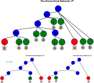
Figure 3: Illustrating the algorithm for a simple hierarchical network.

Figure 4: Illustrating the analysis for hierarchical networks; referred to in the proof of Lemma 2. The square is a node $i$ in $V$ holding object $\beta$, and the hexagon is a fictional $\alpha$-player.

Lemma 2

Consider step $t$ of the algorithm. If $P^{t}$ is an equilibrium for $V\cup W_{t}$, then the following statements hold.

1. For every node $k$ in $V\cup W_{t+1}$, $P^{t+1}_{k}$ is a best response to $P^{t+1}_{-k}$.

2. For every node $k$ in $V\cup W_{t+1}$, $\mu_{k}(P^{t+1})\sqsupseteq_{k}\mu_{k}(P^{t})$.

3. We have $|W_{t+1}|\leq|W_{t}|$. Furthermore, either $|W_{t+1}|<|W_{t}|$ or there exists a node $i$ in $V$ such that $\ \mu_{i}(P^{t+1})\sqsupset_{i}\mu_{i}(P^{t})$.

Proof

Let $\alpha$, $v$, $S$, $i$, and $j$ be defined as described above in step $t$. We first prove the first two lemma’s statements. We let $k$ be any node in $V\cup W_{t+1}$. First, we consider the case that $\mbox{lca}(k,j)$ is an ancestor of $v$. In this case $k$ is not in the subtree rooted at the child $u$ of $v$ that contains $j$. For any object $\gamma$, $\sigma_{k}(P^{t+1}_{-k},\gamma)=\sigma_{k}(P^{t}_{-k},\gamma)$ and $P_{k}^{t+1}=P^{t}_{k}$. Statement 2 for $k$ is implied thus from the fact that $\mu_{k}(P^{t+1})=\mu_{k}(P^{t})$. Since $P^{t}$ is in equilibrium, statement 1 also holds for $k$. We then consider the case that $\mbox{lca}(k,j)$ is a proper descendant of $v$. in this case $k$ is in the subtree rooted at the child $u$ of $v$ that contains $j$. There are two cases.

In the case that $S$ is empty, the fictional $\alpha$-player $j$ is removed. In this way $j$ is not in $W_{t+1}$. Moreover, there is no copy of $\alpha$ in the subtree rooted at $u$. Given that no other object except $\alpha$ is created or removed, $\sigma_{k}(P^{t+1}_{-k},\gamma)=\sigma_{k}(P^{t}_{-k},\gamma)$ for $\gamma\neq\alpha$. The second statement is established for $k$ by the fact that $\mbox{lca}(k,\sigma_{k}(P^{t+1}_{-k},\alpha))=v$ and $\mu_{k}(P^{t+1})=\mu_{k}(P_{t})$. Since $S$ is empty, $\mu_{k}(P^{t})\sqsupseteq_{k}(\alpha,v)$. The first statement for $k$ follows from Lemma 1 and the fact that $P^{t}_{k}$ is in equilibrium such that $P^{t+1}_{k}$ is a best response against $P^{t+1}_{-k}$.

In the second case that $S$ is not empty, we let $i$ be a node in $S$ such that $\mbox{lca}(i,j)$ is lowest among all nodes in $S$, as defined above, $x$ denote $\mbox{lca}(i,j)$, and $P^{t}_{i}$ be equal to $\{\beta\}$, where $\beta\neq\alpha$. From the algorithm it is true that $P^{t+1}_{k}=\{\alpha\}$. We let $k\neq i$ be a node in the subtree rooted at $u$. For any $\gamma\neq\alpha$, $\sigma_{k}(P^{t+1}_{-k},\gamma)=\sigma_{k}(P^{t+1}_{-k},\gamma)$. The second statement is established for $k$ by the fact that since $P_{k}^{t+1}=P_{k}^{t}\neq\{\alpha\}$, we have $\mu_{k}(P^{t+1})=\mu_{k}(P^{t})$. Similarly for node $i$, we have $\mu_{i}(P^{t+1})=(\alpha,v)\sqsupset_{i}\mu_{i}(P^{t})$.

To establish the first statement or any node $k$ in the subtree rooted at $u$ we consider two cases. Let $y$ be the child of $x$ that is an ancestor of $j$ (see Figure 4). In the first case, we let $k$ be in the subtree rooted at $y$. Then, by our choice of $i$, it is true that

$$\mu_{k}(P^{t+1})\sqsupseteq_{k}(\alpha,v)\sqsupseteq_{k}(\alpha,x)=(\alpha,\sigma_{k}(P^{t+1}_{-k},\alpha)),$$

which, by Lemma 1, implies that the first statement holds for $k$. In the second case, we let $k$ be in the subtree rooted at $u$, but not in the subtree rooted at $y$. Again, $\sigma_{k}(P^{t+1}_{-k},\gamma)=\sigma_{k}(P^{t}_{-k},\gamma)$ for $\gamma\neq\alpha$. And for $\alpha$ it is true that

$$(\alpha,\mbox{lca}(k,\sigma_{k}(P^{t+1}_{-k},\alpha)))=(\alpha,\mbox{lca}(k,i))\sqsupseteq_{k}(\alpha,x)\sqsupseteq_{k}\mu_{k}(P^{t})=\mu_{k}(P^{t+1}),$$

which establishes the first statement for $k$ using Lemma 1.

To establish the third statement we use the fact that $|W_{t+1}|\leq|W_{t}|$, which is immediate from the definition of the algorithm’s $t$ step. When $S$ is empty, $|W_{t+1}|<|W_{t}|$ since a fictional player is deleted. When $S$ is nonempty, we have proved above that $\mu_{i}(P^{t+1})\sqsupset_{i}\mu_{i}(P^{t})$. This concludes the proof of the third statement and of the whole lemma.

Theorem 3.1

For hierarchical node preferences, an equilibrium can be found in polynomial time.

Proof

From Lemma 2 and the definition of the algorithm it is straightforward that it returns a valid equilibrium at the termination. We should prove now that the termination is achieved in polynomial time. We consider the potential function given by the sum of $|W_{t}|$ and the sum of the $\mu_{i}(P^{t})$ position in the preorder $\sqsupseteq_{i}$ over all $i$. We notice that $|W_{0}|$ is at most $nm$, where $m$ is the number of objects and $n$ is $|V|$ which is at least the number of internal nodes. Moreover, the initial potential is at most $nm+n^{2}m$ since $|\mbox{{\cal O}}\times I|$ is at most $nm$. From Lemma 2, the potential decreases by at least one in each step and thus the number of steps is at most $nm+n^{2}m$.

We need to also prove that each step can be implemented in polynomial time. In the initialization we add $O(nm)$ fictional players and compute the best response for each node $i\in V$. For the later process, we compare at most $m$ placements for each $k\in V$, i.e. one for each object. During each subsequent step we select a fictional player $j$, we determine whether the set $S$ is nonempty, and if so we compute node $i$ and the updated placement. From this process we only need to explain the computation of $S$ and $i$, where $S$ is the set of all $k$ nodes which are not in equilibrium when a fictional player $j$ is deleted. $S$ is computed as follows: for each node $k\in V$, we replace the current object in its cache by $\alpha$ and add $k$ to $S$. According to the utility, this yields to a more preferable placement. Thus, $S$ can be computed in time polynomial in $n$. To complete the proof of the theorem, we let node $i$ simply be a node in $S$ such that $\mbox{lca}(i,j)$ is lowest among all nodes in $S$. This can also be computed in time polynomial in $n$.

4 A general framework for CSR games with ordinal preferences

In this section, we present a new framework on CSR games with ordinal preferences, to generalize the results that were presented in Section 3 to a broad class of utility functions, and to also enable the study of the existence and complexity of equilibria in more general settings.

Node preference relations. Among all the nodes in $V$, we assume that each node $i\in V$ has a total preorder $\geq_{i}$ and $\geq_{i}$ further satisfies $i\geq_{i}j$ for all $i,j\in V$. A node $i$ prefers $j$ over $k$ if $j\geq_{i}k$, while a node $j$ is the most $i$-preferred in a set $S$ of nodes if $j\in S$ and $j\geq_{i}k$ for all $k\in S$. We let $j=_{i}k$ denote that $j\geq_{i}k$ and $k\geq_{i}j$, while when it is not the case that $k\geq_{i}j$, we denote it by $j>_{i}k$. Notice that $>_{i}$ is a strict weak order and for any $i,j,k\in V$ exactly one of the following three relations hold: 1) $j>_{i}k$, 2) $k>_{i}j$, and 3) $k=_{i}j$. We also extend the $\sigma_{i}(P,\alpha)$ and $\sigma_{i}(P_{-i},\alpha)$ notations such that they denote a most $i$-preferred node holding $\alpha$ in $P$ and $P_{-i}$ respectively, breaking ties arbitrarily.

The access cost function $d$ introduced in Section 2 induces a natural node preference relation: $j>_{i}k$ if $d_{ij}<d_{ik}$, and $j=_{i}k$ if $d_{ij}=d_{ik}$. In fact, as we show in Lemma 3, undirected networks (i.e., when the access cost function is symmetric) are equivalent to acyclic node preference collections. Formally, the collection $\{\geq_{i}:i\in V\}$ is an acyclic node preference collection if there does not exist a sequence of nodes $i_{0},i_{1},\ldots,i_{k-1}$ for an integer $k\geq 3$ such that $i_{(j-1)\bmod k}>_{i_{j}}i_{(j+1)\bmod k}$ for all $0\leq j<k$.

Lemma 3

Any undirected network yields an acyclic node preference collection. For any acyclic node preference collection, we can compute, in polynomial time, symmetric cost functions that are consistent with the node preferences.

Proof

Let $d$ denote a symmetric access cost function over the set $V$ of nodes. For a given node $i\in V$, we have $j\geq_{i}k$ iff $d_{ij}\leq d_{ik}$. We now argue that the collection $\{\geq_{i}:i\in V\}$ is acyclic. Suppose, for the sake of contradiction, that there exists a sequence of nodes $i_{0},i_{1},\ldots,i_{k-1}$ for an integer $k\geq 3$ such that $i_{(j-1)\bmod k}>_{i_{j}}i_{(j+1)\bmod k}$ for all $0\leq j<k$. It then follows that:

$$d_{i_{j}i_{(j-1)\bmod k}}<d_{i_{j}i_{(j+1)\bmod k}}\mbox{ for }0\leq j<k.$$

Since $d$ is symmetric, we obtain

$$d_{i_{j}i_{(j-1)\bmod k}}<d_{i_{(j+1)\bmod k}i_{j}}\mbox{ for }0\leq j<k,$$

which is a contradiction, since $d_{i_{0}i_{(k-1)}}<d_{i_{1}i_{0}}<\dots<d_{i_{(k-1)}i_{0}}=d_{i_{0}i_{(k-1)}}$.

Given an acyclic collection of node preferences, we compute an associated access cost function $d$ in polynomial time as follows. We construct a directed graph $G$ over the set $U$ of all unordered pairs $(i,j):i,j\in V$, $i\neq j$. There is a directed edge from node $(i,j)$ to $(i,k)$ if and only if $k\geq_{i}j$. Since the collection $\{\geq_{i}:i\in V\}$ is acyclic, $G$ is a dag. We compute the topological ordering $\pi:U\rightarrow\mathbb{Z}$; thus, we have $\pi((i,j))<\pi((k,\ell))$ whenever there is a directed path from $(i,j)$ to $(k,\ell)$. Setting $d_{ij}$ to be $\pi((i,j))$ gives us the desired undirected network.

Utility preference relations. Each node in our game-theoretic model attaches a utility to each global placement. In our general definition a large class of utility functions it is considered simultaneously. Instead of defining a numerical utility function, we let the utility at each node $i$ be a total preorder $\succeq_{i}$ among the set of all global placements. The $\succ_{i}$ and $=_{i}$ notations over global placements are defined analogously. We require that $\succeq_{i}$, for each $i\in V$, satisfies the following two basic conditions:

• Monotonicity: If for any two global placements $P$ and $Q$, for each object $\alpha$, and each node $q$ with $\alpha\in Q_{q}$, there exists a node $p$ with $\alpha\in P_{p}$ and $p\geq_{i}q$, then $P\succeq_{i}Q$.

• Consistency: Let two global placements $(P_{i},P_{-i})$ and $(Q_{i},Q_{-i})$ such that for each object $\alpha\in P_{i}\cup Q_{i}$, if $p$ (resp. $q$) is a most $i$-preferred node in $V\setminus\{i\}$ holding $\alpha$, i.e. $\alpha\in P_{p}$ (resp. $\alpha\in Q_{q}$), then $p=_{i}q$. If $(P_{i},P_{-i})\succ_{i}(Q_{i},P_{-i})$, then $(P_{i},Q_{-i})\succeq_{i}(Q_{i},Q_{-i})$.

In words, the monotonicity condition says that for any node, if all the objects in a placement are placed at nodes that are at least as preferred as in another placement, then the node prefers the former placement at least as much as the latter. The consistency condition says that the preference for a node to store one set of objects instead of another is entirely a function of the set of most preferred other nodes that together hold these objects. For instance, if a node $i$ with unit capacity prefers to store $\alpha$ over $\beta$ in a scenario where the most $i$-preferred node (other than $i$) storing $\alpha$ (resp. $\beta$) is $j$ (resp. $k$), then $i$ prefers to store $\alpha$ at least as much as $\beta$ in any other situation where the most $i$-preferred node (other than $i$) storing $\alpha$ (resp. $\beta$) is $j$ (resp. $k$).

Generality of the conditions. We note that many standard utility functions defined for replica placement problems Chun et al (2004); Laoutaris et al (2007); Pollatos et al (2008), including the sum and max functions, satisfy the monotonicity and consistency conditions. Indeed, any utility function that is an $L_{p}$ norm, for any $p$, over the costs for the individual objects, also satisfies the conditions. Furthermore, since the monotonicity and consistency conditions apply to the individual utility functions, our model allows the different nodes to adopt different types of utilities, as long as each separately satisfies the two conditions.

Binary object preferences. One of the utility preference relations classes we study is based on binary object preferences. Assume that each node $i$ is equally interested in an objects set $S_{i}$ and it does not have any interest in the other objects. Then, $\tau_{i}(P)$ will denote the $|S_{i}|$-length sequence of the $\sigma_{i}(P,\alpha)$, such that $\alpha\in S_{i}$ and it is in non-increasing order based on the $\geq_{i}$ relation. In this setup the consistency condition can be further strengthened to the binary consistency term: for any placements $P=(P_{i},P_{-i})$ and $Q=(Q_{i},Q_{-i})$ with $P_{-i}=Q_{-i}$, we let $P\succeq_{i}Q$ if and only if for $1\leq k\leq|S_{i}|$, the $k^{th}$ component of $\tau_{i}(P)$ is at least as $i$-preferred as the $k^{th}$ component of $\tau_{i}(Q)$.

CSR Games. We let a CSR game be a tuple $(V,\mbox{{\cal O}},\{\geq_{i}\},\{\succeq_{i}\})$ in the general axiomatic framework. A pure Nash equilibrium in a CSR game instance is a global placement $P$ such that there is no placement $Q_{i}$ for which $(Q_{i},P_{-i})\succ_{i}(P_{i},P_{-i})$, for each $i\in V$.

To further analyse the complexity results, a definition of a game instance specification is required. We first specify the set $V$, the node cache capacities, and an enumerated list of object names O. For each node $i\in V$, we specify $i$’s preference relation $\geq_{i}$ succinctly by a set of at most $\binom{n}{2}$ bits. However, the utility preference relation $\succeq_{i}$ is over a potentially exponential number of placements in terms of $n$, $m$, and cache sizes. We further assume that the utility preference relations are specified by an efficient algorithm, which we denote as utility preference oracle, that takes as input a node $i$, and two global placements $P$ and $Q$, and returns whether $P\succeq_{i}Q$. For the sum, max, and $L_{p}$-norm utilities, the utility preference oracle simply computes the relevant utility function. For binary object preferences, the binary consistency condition yields an oracle which is polynomial in the number of nodes, objects, and cache sizes.

Unit cache capacity. We now argue that the unit cache capacity assumption of Section 2 continues to hold without loss of generality. Consider a set $V$ of nodes in which the cache of node $i$ can store $c_{i}$ objects. Let $V^{\prime}$ denote a new set of nodes which contains, for each node $i$ in $V$, new nodes $i_{1},i_{2},\ldots,i_{c_{i}}$, i.e., one new node for each unit of the cache capacity of $i$. We set the node preferences as follows: for all $i,i^{\prime},j\in V$, $1\leq f,\ell\leq c_{j}$, $1\leq k,k^{\prime}\leq c_{i}$, we have $i_{k}\geq_{j_{\ell}}i^{\prime}_{k^{\prime}}$ whenever $i\geq_{j}i^{\prime}$, and $j_{f}=_{i_{k}}j_{\ell}$.

We consider an obvious onto mapping $f$ from placements in $V^{\prime}$ to those in $V$. Given placement $P^{\prime}$ for $V^{\prime}$, we set $f(P^{\prime})=P$ where $P_{i}=\cup_{1\leq k\leq c_{i}}P^{\prime}_{i_{k}}$. This mapping naturally defines the utility preference relations for the node set $V^{\prime}$. In particular, for any $i\in V$ and $1\leq k\leq c_{i}$, $P^{\prime}\succeq_{i_{k}}Q^{\prime}$ whenever $f(P^{\prime})\succeq_{i}f(Q^{\prime})$. We also note that $f$ is computable in time polynomial in the number of nodes and the sum of the cache capacities. It is easy to verify that the utility preference relation $\succeq_{i_{k}}$ for all $i_{k}\in V^{\prime}$ satisfies the monotonicity and consistency conditions. Furthermore, $P^{\prime}$ is an equilibrium for $V^{\prime}$ if and only if $f(P^{\prime})$ is an equilibrium for $V$; this together with the onto property of the mapping $f$ gives us the desired reduction.

5 Existence of equilibria in the general framework

In this section, we establish the existence of equilibria for several CSR games under the general framework of CSR games with ordinal preferences that we introduced in Section 4. First, we extend the sum utility function results on hierarchical networks to the general framework (Section 5.1). Next, we show that CSR games on undirected networks and binary object preferences are potential games (Section 5.2). Finally, when there are only two objects in the system, we use the technique of fictional players to give a polynomial-time construction of equilibria for CSR games on undirected networks (Section 5.3).

5.1 Hierarchical networks

We fist show that the polynomial time algorithm which was introduced in Section 3 holds also for the general framework of CSR games with ordinal preferences. A hierarchical network, as defined in the general framework, is a tree $T$ whose leaves set is the node set $V$ and the node preference relation $\geq_{i}$ is $j\geq_{i}k$ if $\mbox{lca}(i,j)$ is a descendant of $\mbox{lca}(i,k)$. This hierarchical network structure and each node’s $i$ pair-preference relations $\sqsupseteq_{i}$, determine completely the analysis of the algorithm introduced in Section 3. The latter were defined for the sum utility function. Extending our analysis to the general framework, requires a new preference relation derivation and the establishment of Lemma’s 1 analogue, which we present next for arbitrary utility preference relations that satisfy the monotonicity and consistency properties.

Pair preference relations. For any utility preference relation $\succeq_{i}$ that satisfies the monotonicity and consistency conditions, we define a strict weak order $\sqsupset_{i}$ on $\mbox{{\cal O}}\times A_{i}$, where $A_{i}$ is the set of $i$’s proper ancestors in $T$.

1. We let $(\alpha,v)\sqsupset_{i}(\alpha,w)$ hold whenever $v$ is a proper ancestor of $w$, for each object $\alpha$, node $i$, and proper $i$’s ancestors $v$ and $w$.

2. Considering distinct objects $\alpha,\beta$ and nodes $i,j,k$ with $j,k\neq i$, we let ${\cal P}$ be the set of global placements $P$, such that $j$ (resp. $k$) is a most $i$-preferred node in $V\setminus\{i\}$ holding $\alpha$ (resp. $\beta$) in $P_{-i}$. If there exist global placements $P=(\{\alpha\},P_{-i})$ and $Q=(\{\beta\},P_{-i})$ in ${\cal P}$ with $P\succ_{i}Q$, then $(\alpha,\mbox{lca}(i,j))\sqsupset_{i}(\beta,\mbox{lca}(i,k))$.

In words, item 1 says that $i$’s preference for keeping $\alpha$ in its cache increases as the most $i$-preferred node holding $\alpha$ becomes less preferred (or “moves farther away”). In item 2, $(\alpha,v)\sqsupset_{i}(\beta,w)$ means that if $i$ needs to place either $\alpha$ or $\beta$ in its cache, and the least common ancestor of $i$ and the most $i$-preferred node in $V\setminus\{i\}$ holding $\alpha$ (resp., $\beta$) is $v$ (resp., $w$), then $i$ prefers to store $\alpha$ over $\beta$. The strict weak order $\sqsupset_{i}$ induces a total preorder $\sqsupseteq_{i}$ as follows: $(\alpha,v)\sqsupseteq_{i}(\beta,w)$ if it is not the case that $(\beta,v)\sqsupset_{i}(\alpha,w)$. We similarly define $=_{i}$: $(\alpha,v)=_{i}(\beta,w)$ if $(\alpha,v)\sqsupseteq_{i}(\beta,w)$ and $(\beta,v)=_{i}(\alpha,w)$.

Lemma 4

For each $i$, $\sqsupset_{i}$ as given above, is a well-defined strict weak order.

Proof

We need to ensure the well-definedness of part 2 of the definition of pair preference relations. That is, we need to show that for any placements $P_{-i}$ and $Q_{-i}$ such that a most $i$-preferred node in $P_{-i}$ holding $\alpha$ (resp., $\beta$) is also a most $i$-preferred node in $Q_{-i}$, it is impossible that $(\{\alpha\},P_{-i})\succ_{i}(\{\beta\},P_{-i})$ and $(\{\beta\},Q_{-i})\succ_{i}(\{\alpha\},Q_{-i})$ both hold. This directly follows from the consistency condition for utility preference relations.

The reflexivity and transitivity of $\sqsupseteq_{i}$ are immediate from the definitions and the reflexivity and transitivity of $\succeq_{i}$. Finally, to ensure the well-definedness of the strict preorder $\sqsupset_{i}$, we also have to show that there is no collection of pairs $(\alpha_{j},v_{j})$, $0\leq j<\ell$ for some integer $\ell>1$, such that $(\alpha_{j},v_{j})\sqsupset_{i}(\alpha_{j+1\bmod\ell},v_{j+1\bmod\ell})$ for $0\leq j<\ell$. To see this, it is sufficient to note that if $(\alpha,v)\sqsupset_{i}(\alpha^{\prime},v^{\prime})$ then for all placements $P$ and $P^{\prime}$ such that $P_{-i}=P^{\prime}_{-i}$ and the least common ancestor of $i$ and the most $i$-preferred node in $V\setminus\{i\}$ that holds $\alpha$ (resp. $\alpha^{\prime}$) is $v$ (resp. $v^{\prime}$) we have $P\succ_{i}P^{\prime}$. So any cycle in the strict preorder $\sqsupset_{i}$ implies a cycle in $\succ_{i}$, yielding a contradiction.

Analogous to Lemma 1, we can express the best response of any player in hierarchical networks as follows. For any global placement $P=(\{\alpha\},P_{-i})$, assume that $j$ (resp. $k$) is a most $i$-preferred node holding object $\alpha$ (resp. $\beta$) in $P_{-i}$, and $(\{\beta\},P_{-i})\succ_{i}(\{\alpha\},P_{-i})$, i.e., for node $i$, storing $\beta$ is a better response to $P_{-i}$ than storing $\alpha$. Then the following Lemma holds.

Lemma 5

For any global placement $P=(\{\alpha\},P_{-i})$, $(\beta,\mbox{lca}(i,k))\sqsupset_{i}(\alpha,\mbox{lca}(i,j))$. Furthermore, $\{\alpha\}$ is a best response to $P_{-i}$, where $\alpha$ maximizes $(\gamma,\mbox{lca}(i,\sigma_{i}(P_{-i},\gamma)))$, over all objects $\gamma$, according to $\sqsupseteq_{i}$.

Proof

The first statement of the lemma directly follows from item 2 of the definition of pair preference relations. We establish the second statement by contradiction. Suppose that for node $i$, $\{\beta\}$ is a better response to $P_{-i}$ than $\{\alpha\}$. Then, we have $(\{\beta\},P_{-i})\succ_{i}(\{\alpha\},P_{-i})$, which, by item 2 of the definition of pair preference relations, implies that $(\beta,\mbox{lca}(i,\sigma_{i}(P_{-i},\beta)))\sqsupset_{i}(\alpha,\mbox{lca}(i,\sigma_{i}(P_{-i},\alpha)))$, a contradiction to the choice of $\alpha$.

The remainder of the analysis for hierarchical networks (Lemma 2 and Theorem 3.1) follows as before, invoking Lemma 5 instead of Lemma 1.

5.2 Undirected networks with binary object preferences

Let $d$ be a symmetric cost function for an undirected network over the node set $V$. From the binary object preferences definition for each node $i$ we are given an object set $S_{i}$ in which $i$ is equally interested. We prove the existence of equilibria via a potential function argument. Given a placement $P$, we let $\Phi_{i}(P)=d_{ij}$, where $j$ is the most $i$-preferred node in $V-\{i\}$ holding the object in $P_{i}$. We introduce the potential function $\Phi$: $\Phi(P)=(\Phi_{0},\Phi_{i_{1}}(P),\Phi_{i_{2}}(P),\ldots,\Phi_{i_{n}}(P))$, where $\Phi_{0}$ is the number of nodes $i$ such that $P_{i}\subseteq S_{i}$, and $\Phi_{i_{j}}(P)\leq\Phi_{i_{j+1}}(P)$, $\forall j$, where $V=\{i_{1},i_{2},\ldots,i_{n}\}$. We prove that $\Phi$ is an increasing potential function, i.e. after any better response step, $\Phi$ increases in lexicographical order.

Let $P=(P_{i},P_{-i})$ be an arbitrary global placement. Assume that $P_{i}=\{\alpha\}$ and $j$ is the most $i$-preferred node in $P_{-i}$ holding $\alpha$. Consider any better response step, from placement $P$ to $Q=(Q_{i},P_{-i})$, where $Q_{i}=\{\beta\}$. Clearly $\beta\in S_{i}$. We consider two cases. First, suppose $\alpha\notin S_{i}$ and $\beta\in S_{i}$. Then, $\Phi_{0}$ increases, and so does the potential. The second case is where $\alpha,\beta\in S_{i}$. Let $k$ be the most $i$-preferred node in $P_{-i}$ holding $\beta$. In this case, $\Phi_{0}$ does not change. However, since this is a better response step of $i$, $j>_{i}k$, implying that $d_{ik}>d_{ij}$ and hence $\Phi_{i}(Q)>\Phi_{i}(P)$. Consider any other node $j$. If $j$ holds any object $\gamma$ other than $\beta$, since no new copy of $\gamma$ has been added, $\Phi_{j}(Q)\geq\Phi_{j}(P)$. It remains to consider the case where $j$ holds $\beta$. If $S$ is the set of nodes in $V\setminus\{j\}$ holding $\beta$ in $P_{-j}$, then $S\cup\{i\}$ is the set of nodes in $V\setminus\{j\}$ holding $\beta$. Thus, $\Phi_{j}(Q)=\min\{\Phi_{j}(P),d_{ji}\}\geq\min\{\Phi_{j}(P),\Phi_{i}(Q)\}$. This also means that $\Phi_{j}(P)$ appears later in the sorted order than $\Phi_{i}(P)$ and $\Phi_{j}(Q)$ appears no earlier in the sorted order than $\Phi_{i}(Q)$. Hence, $\Phi(Q)$ is lexicographically greater than $\Phi(P)$. This establishes that for undirected networks with binary object preferences, the resulting CSR game is a potential game, and hence also in PLS Johnson et al (1988).

5.3 Undirected networks with two objects

In the case of an undirected network with two objects we provide a polynomial-time algorithm to compute an equilibrium. We use the fictional player technique that was introduced in Section 5.1. In the beginning a set of fictional players are introduced to serve the two objects in the network at zero cost from each node. In each subsequent step, the fictional players are progressively moved “further” away, in a way that at each instance the equilibrium is ensured. The whole set of fictional players are completely removed when they are at the least preferred cost from all the nodes, yielding finally to an equilibrium for the original network.

Suppose we are given a undirected network with access cost function $d$. Also let ${\cal D}$ be the set $\{0,\ell_{1},\ell_{2},\ldots,\ell_{r}\}$ of all access costs between nodes in the system in increasing order; that is, $\ell_{1}=\min_{i,j}d_{ij}$ and $\ell_{r}=\max_{i,j}d_{ij}$ and $\ell_{i}<\ell_{i+1}$ for all $1\leq i<r$.

Fictional player. For an object $\alpha$, a fictional $\alpha$-player is a new node that will store $\alpha$ in every equilibrium; an fictional $\alpha$-player prefers storing $\alpha$ over any other object. We denote by $srv_{\alpha}(\ell)$ the fictional $\alpha$-player which is at access cost $\ell$ from every node in $V$.

The algorithm.

Initialization. Assuming that there are two objects $\alpha$ and $\beta$ in the system, we initially set up a fictional $\alpha$-player $srv_{\alpha}(0)$ and $\beta$-player $srv_{\beta}(0)$ at access cost $0$ from each node in $V$, which does not affect the actual distance between nodes. We let nodes replicate their most preferred object and access the other without any access cost from the corresponding fictional player. This placement is obviously an equilibrium.

Step $t$ of algorithm. Fix an equilibrium $P$ for the node set $V\cup\{srv_{\alpha}(\ell_{t})\}\cup\{srv_{\beta}(\ell_{t})\}$. We describe one step of the algorithm which computes a new set of fictional players $srv_{\alpha}(\ell_{t+1})$ and $srv_{\beta}(\ell_{t+1})$ and a new placement $P^{\prime}$ such that $P^{\prime}$ is an equilibrium for the node set $V\cup\{srv_{\alpha}(\ell_{t+1})\}\cup\{srv_{\beta}(\ell_{t+1})\}$. We first remove the $\alpha$-player $srv_{\alpha}(\ell_{t})$ from the system and instead we add $srv_{\alpha}(\ell_{t+1})$. If there do not exist nodes that want to deviate we are done. Otherwise, assume that there exists a node $i$ that wants to deviate from its strategy. Since the most $i$-preferred node holding $\beta$ in $V\cup\{srv_{\alpha}(\ell_{t})\}\cup\{srv_{\beta}(\ell_{t})\}$ remains the same in $V\cup srv_{\alpha}(\ell_{t+1})\cup srv_{\beta}(\ell_{t})$, $i$ is not holding object $\alpha$. Thus the only nodes that may want to deviate are those that are holding object $\beta$. We argue that if we let $i$ to deviate from $\beta\in P_{i}$ to $\alpha\in P^{\prime}_{i}$, there is no node $j\in V\setminus\{i\}$ that gets affected by $i$’s deviation. Consider the following two cases:

• If a node $j$ has access cost at most $\ell_{t}$ from $i$, then $\beta\in P_{j}$. Otherwise, if $\alpha\in P_{j}$, $srv_{\alpha}(\ell_{t})$ would not be the most $i$-preferred node holding $\alpha$ and thus $i$ would not be affected by any change of $\alpha$-players. Thus there does not exist any node $j\in V\setminus\{i\}$ with access cost at most $\ell_{t}$ from $i$, such that $\alpha\in P_{j}$, and as we showed above $\alpha\in P^{\prime}_{j}$.

• If a node $j$ has access cost at least $\ell_{t+1}$ from $i$, then $P_{j}=P^{\prime}_{j}$. Because of the $\alpha$-player $srv_{\alpha}(\ell_{t+1})$ and the $\beta$-player $srv_{\beta}(\ell_{t})$, $i$ would never be the $j$-most preferred node in $P^{\prime}$.

We then remove the $\beta$-player $srv_{\beta}(\ell_{t})$ from the system and instead we add $srv_{\beta}(\ell_{t+1})$. Using a similar argument as above, we obtain a new equilibrium at the end of this step.

Theorem 5.1

For undirected networks with two objects, an equilibrium can be found in polynomial time.

Proof

An initial placement $P$, where we have the set of fictional players $srv_{\alpha}(0)$ and $srv_{\beta}(0)$ in the system, is obviously an equilibrium. It is immediate from our argument above that at termination the algorithm returns a valid equilibrium.

The size of the set ${\cal D}$ is at most ${n\choose 2}$ which is at most $n^{2}$. In each step $t$ at most $n$ nodes may want to deviate from their strategy, since we showed above that if a node deviates once in a step, it will not deviate again during the same step. Thus, the total number of deviations in the algorithm is at most $n^{3}$.

6 Non-Existence of equilibria in CSR games and the associated decision problem

In this section, we show that the classes of games studied in Section 5 are essentially the only games where equilibria are guaranteed to exist. We identify the most basic CSR games where equilibria may not exist, and study the complexity of the associated decision problem.

6.1 NP-Completeness

We first show that it is NP-hard to determine whether a given CSR game has an equilibrium even when the utility preference relations are based on the sum utility function and either the number of objects is small or the object preferences are binary. Some simple network examples appear in Fig. 5 (middle and right)–the networks are described in details after Theorem 6.1–showing that there does not exist an equilibrium in these configurations (proved in the second part of Theorem 6.2 and 6.3). The NP-hardness proof is by a polynomial-time reduction from 3SAT Garey and Johnson (1979). Each reduction is built on top of a gadget which has an equilibrium if and only if a specified node holds a certain object. Several copies of these gadgets are then put together to capture the given 3SAT formula.

Theorem 6.1

The problem of determining whether a CSR instance has an equilibrium is in NP even if one of these three restrictions hold: (a) the number of objects is two; (b) the object preferences are binary and number of objects is three; (c) the network is undirected and the number of objects is three.

The membership in NP is immediate, since one can determine in polynomial time whether a given global placement is an equilibrium. The remainder of the proof focuses on the hardness reduction from 3SAT.

Given a 3SAT formula $\phi$ with $n$ variables $x_{1}$, $x_{2}$, $\ldots$, $x_{n}$ and $k$ clauses $c_{1}$, $c_{2}$, $\ldots$, $c_{k}$, we construct a CSR instance as follows. For each variable $x_{i}$ in $\phi$, we introduce two variable nodes $X_{i}$ and $\bar{X}_{i}$. We set $d_{X_{i}\bar{X}_{i}}$ and the symmetric $d_{\bar{X}_{i}X_{i}}$ to be $0.5$, where $d$ is the underlying access cost function. For each clause $c_{j}$ we introduce a clause node $C_{j}$. Assuming that $\ell_{j,r}$ for $r\in\{1,2,3\}$, are the three literals of the $c_{j}$ clause in formula $\phi$, we set $d_{C_{j}L_{j,r}}$ and $d_{L_{j,r}C_{j}}$ to be $1$, where $L_{j,r}$ is the corresponding variable node. We also introduce a gadget $G$ illustrated in Figure 5 (middle and right), consisting of nodes $S$, $A$, $B$, and $C$. We set the access cost $d_{SC_{i}}$ and the symmetric $d_{C_{i}S}$, for all $1\leq i\leq k$ between node $S$ and all clause nodes to be $2$. The general construction is illustrated in Figure 5 (left).

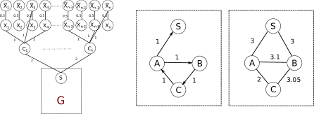
Figure 5: Left: instance of the construction for the undirected case proof of NP-Hardness, where $\phi=(x_{1}\vee\bar{x_{3}}\vee x_{4})\wedge\ldots\wedge(x_{n-3}\vee x_{n-1}\vee\bar{x_{n}})$. Middle and right: gadget G for the directed and the undirected case

Directed networks with two objects. We set the access costs $d_{AS}=d_{AB}=d_{BC}=d_{CA}=1$, and the server node, which stores a fixed copy of two objects $\alpha$ and $\beta$, at access cost $d_{srv}=10$ from all nodes in $V$. We also set the weights of the variable nodes $r_{x_{i}}(\alpha)=r_{\bar{x}_{i}}(\alpha)=r_{x_{i}}(\beta)=r_{\bar{x}_{i}}(\beta)=1$, the weights of the clause nodes $r_{C_{i}}(\alpha)=0.85$ and $r_{C_{i}}(\beta)=1$, for all $1\leq i\leq k$. Finally, we set the weights of the nodes in the G gadget $r_{S}(\alpha)=0.85$, $r_{S}(\beta)=r_{A}(\beta)=r_{B}(\alpha)=r_{B}(\beta)=r_{C}(\alpha)=r_{C}(\beta)=1$ and $r_{A}(\alpha)=0.7$. We refer to this CSR instance as $I_{1}$.

Undirected networks with three objects. We set the access costs $d_{AS}=d_{BS}=3$, $d_{AB}=3.1$, $d_{BC}=3.05$, and $d_{CA}=2$; while symmetry holds. The server node, which stores a fixed copy of three objects $\alpha$, $\beta$, and $\gamma$, is at access cost $d_{srv}=5$ from all nodes in $V$. We set the weights of the clause nodes $r_{x_{i}}(\alpha)=r_{\bar{x}_{i}}(\alpha)=r_{x_{i}}(\beta)=r_{\bar{x}_{i}}(\beta)=1$, the weights of the clause nodes $r_{C_{i}}(\alpha)=0.85$ and $r_{C_{i}}(\beta)=1$, for all $1\leq i\leq k$. Finally, we set the weight of the nodes in the G gadget $r_{S}(\alpha)=0.85$, $r_{S}(\beta)=r_{A}(\alpha)=r_{B}(\beta)=r_{C}(\beta)=1$, $r_{A}(\gamma)=2$, $r_{B}(\gamma)=0.9837$, and $r_{C}(\gamma)=1.6$. All the remaining weights are set to $0$. We refer to this CSR instance as $I_{2}$.

Lemma 6

A variable node $X_{i}$ holds object $\alpha$ (resp., $\beta$) if and only if node $\bar{X}_{i}$ holds object $\beta$ (resp., $\alpha$).

Proof

The proof is immediate, since $\bar{X}_{i}$ (resp., $X_{i}$) is $X_{i}$’s (resp., $\bar{X}_{i}$’s) nearest node, and both $X_{i}$ and $\bar{X_{i}}$ are interested equally in $\alpha$ and $\beta$.

Lemma 7

Clause node $C_{i}$ holds object $\alpha$ if and only if its variable nodes $L_{i,j}$, for $j\in\{1,2,3\}$ hold object $\beta$.

Proof

First, assume that $L_{i,j}$, for $j\in\{1,2,3\}$ hold $\beta$. These nodes are $C_{i}$’s nearest nodes holding $\beta$. By Lemma 6 we know that nodes $\bar{L}_{i,j}$, for $j\in\{1,2,3\}$ hold $\alpha$, and they are $C_{i}$’s nearest nodes holding $\alpha$. Node’s $C_{i}$ cost for holding $\alpha$ and accessing $\beta$ from $L_{i,j}$, for $j\in\{1,2,3\}$, is $r_{C_{i}}(\beta)d_{C_{i}L_{i,j}}=1$; while the cost for holding $\beta$ and accessing $\alpha$ from $\bar{L}_{i,j}$, for $j\in\{1,2,3\}$, is $r_{C_{i}}(\alpha)d_{C_{i}\bar{L}_{ij}}=1.275$. Obviously, node $C_{i}$ prefers to replicate $\alpha$.

Now assume that at least one of the nodes $\bar{L}_{i,j}$, for $j\in\{1,2,3\}$ holds $\alpha$. These nodes are $C_{i}$’s nearest nodes holding $\alpha$. Also, by Lemma 6, $C_{i}$’s nearest nodes holding $\beta$ are all the remaining nodes from the set $L_{i,j}$, $\bar{L_{i,j}}$, for $j\in\{1,2,3\}$, that don’t hold $\alpha$. Node’s $C_{i}$ cost for holding $\beta$ and accessing $\alpha$ from $L_{i,j}$, for $j\in\{1,2,3\}$, is $r_{C_{i}}(\alpha)d_{C_{i}L_{i,j}}=0.85$; while the cost for holding $\alpha$ and accessing $\beta$ from node $\bar{L}_{i,j}$ (resp., $L_{i,j}$), is $r_{C_{i}}(\beta)d_{C_{i}\bar{L}_{i,j}}=1.5$ (resp., $r_{C_{i}}(\beta)d_{C_{i}L_{i,j}}=1$). Obviously, in any case node $C_{i}$ prefers to replicate $\beta$.

Lemma 8

Node $S$ holds object $\alpha$ if and only if all clause nodes $C_{1},\ldots,C_{k}$ hold object $\beta$.

Proof

First, assume that $C_{1},\ldots,C_{k}$ are holding $\beta$. These nodes are $S$’s nearest nodes holding $\beta$. Also by Lemma 7, $S$’s nearest node holding $\alpha$ is at least one of $L_{i,j}$ nodes, where $i\in[1,k],j\in\{1,2,3\}$. The cost for $S$ holding $\alpha$ and accessing $\beta$ from a node $C_{i},i\in[1,k]$, is $r_{S}(\beta)d_{SC_{i}}=2$; while the cost for holding $\beta$ and accessing $\alpha$ from $L_{i,j}$, where $i\in[1,k],j\in\{1,2,3\}$, is $r_{S}(\alpha)d_{SL_{i,j}}=2.55$. Obviously, node $S$ prefers to replicate $\alpha$.

Now assume that at least one of $C_{1},\ldots,C_{k}$ holds $\alpha$. These nodes are $S$’s nearest node holding $\alpha$. Also $S$’s nearest node holding $\beta$, due to Lemma 7 is one of $L_{i,j}$, where $i\in[1,k],j\in\{1,2,3\}$. The cost for holding $\beta$ and accessing $\alpha$ from a node $C_{i}$, is $r_{S}(\alpha)d_{SC_{i}}=1.7$; while the cost for holding $\alpha$ and accessing $\beta$ from a node $L_{ij}$, where $j\in\{1,2,3\}$, is $r_{S}(\beta)d_{SL_{i,j}}=3$. Obviously, in any case node $S$ prefers to replicate $\beta$.

Theorem 6.2

The CSR instance $I_{1}$ has an equilibrium if and only if node $S$ holds object $\alpha$.

Proof

First, assume that $S$ is holding $\alpha$. By Lemma 8 nodes $C_{1},\ldots,C_{k}$ hold object $\beta$, and by Lemma 7 at least one of nodes $L_{i,j}$, for $j\in\{1,2,3\}$ for each node $C_{i},i\in[1,k]$, holds object $\alpha$, and the corresponding $\bar{L}_{i,j}$ is holding object $\beta$. We claim that the placement where $A$ holds $\beta$, $B$ holds $\beta$, and $C$ holds $\alpha$, is a pure Nash equilibrium. We prove this by showing that none of these nodes wants to deviate from their strategy.

Node $A$ does not want to deviate since its cost for holding object $\beta$ and accessing $\alpha$ from $A$’s nearest node $S$, is $r_{A}(\alpha)d_{AS}=0.7$; while the cost for holding object $\alpha$ and accessing $\beta$ from $A$’s nearest node $B$, is $r_{A}(\alpha)d_{AB}=1$. Node $B$ does not want to deviate since its cost for holding object $\beta$ and accessing $\alpha$ from $B$’s nearest node $C$, is $r_{B}(\alpha)d_{BC}=1$; while the cost for holding object $\alpha$ and accessing $\beta$ from $B$’s nearest node $A$, is $r_{B}(\beta)d_{BA}=2$. Node $C$ does not want to deviate since its cost for holding object $\alpha$ and accessing $\beta$ from $C$’s nearest node $A$, is $r_{C}(\beta)d_{CA}=1$; while the cost for holding object $\beta$ and accessing $\alpha$ from $C$’s nearest node $S$, is $r_{C}(\alpha)d_{CS}=2$. Also note that none of $S,C_{1},\ldots,C_{k},L_{ij},\bar{L}_{ij}$ for $i\in[1,k],j\in\{1,2,3\}$ is getting affected of the objects been held by the gadget nodes.

Now assume that node $S$ holds object $\beta$. We are going to prove that for every possible placement over nodes $A$, $B$, and $C$, at least one node wants to deviate from its strategy. Consider the following cases:

• Nodes $A$, $B$, and $C$ hold object $\alpha$: Node $B$ (resp., $C$) wants to deviate, since the cost for holding object $\alpha$ and accessing $\beta$ from $B$’s (resp., $C$’s) nearest node $S$, is $r_{B}(\beta)d_{BS}=3$ (resp., $r_{C}(\beta)d_{CS}=2$); while the cost for holding object $\beta$ and accessing $\alpha$ from $B$’s nearest node $A$, is $r_{B}(\beta)d_{BA}=2$ (resp., $r_{C}(\beta)d_{CA}=1$).

• Two nodes hold object $\alpha$ and the third holds $\beta$: In the case where $A$ and $B$ hold $\alpha$, $A$ wants to deviate since the cost while holding $\alpha$ and accessing $\beta$ from $A$’s nearest node $S$ is $r_{A}(\beta)d_{AS}=1$; while the cost for holding $\beta$ and accessing $\alpha$ from $A$’s nearest node $B$ is $r_{A}(\alpha)d_{AB}=0.7$. In the case where $A$ and $C$ hold $\alpha$, then $C$ wants to deviate since the cost while holding $\alpha$ and accessing $\beta$ from $C$’s nearest node $B$ is $r_{C}(\beta)d_{CB}=2$; while the cost for holding $\beta$ and accessing $\alpha$ from $C$’s nearest node $A$ is $r_{C}(\alpha)d_{CA}=1$. In the case where $B$ and $C$ hold $\alpha$, $B$ wants to deviate since the cost while holding $\alpha$ and accessing $\beta$ from $B$’s nearest node $A$ is $r_{B}(\beta)d_{BA}=2$; while the cost for holding $\beta$ and accessing $\alpha$ from $B$’s nearest node $C$ is $r_{B}(\alpha)d_{BC}=1$.

• One node holds $\alpha$: If $A$ (resp., $B$, or $C$) holds $\alpha$, $B$ (resp., $C$, $A$) wants to deviate since the cost while holding $\beta$ and accessing $\alpha$ from $B$’s (resp., $C$’s, or $A$’s) nearest node $A$ (resp., $B$, or $C$) is $r_{B}(\alpha)d_{BA}=2$ (resp., $r_{C}(\alpha)d_{CB}=2$, or $r_{A}(\alpha)d_{AC}=1.4$); while the cost for holding $\alpha$ and accessing $\beta$ from $B$’s (resp., $C$’s, or $A$’s) nearest node $C$ (resp., $A$, or $B$), is $r_{B}(\beta)d_{BC}=1$ (resp., $r_{C}(\beta)d_{CA}=1$, or $r_{A}(\beta)d_{AB}=1$).

• Nodes $A$, $B$, and $C$ hold $\beta$: All of them want to deviate. Node $A$ wants to deviate since the cost while holding $\beta$ and accessing $\alpha$ from $A$’s nearest node $C_{i}$, for some $i\in[1,k]$, is $r_{A}(\beta)d_{AC_{i}}=3$; while the cost for holding $\beta$ and accessing $\alpha$ from $A$’s nearest node $S$ is $r_{A}(\alpha)d_{AS}=0.7$. Similar proof holds for nodes $B$ and $C$.

Obviously the system does not have a pure Nash equilibrium, which completes the proof.

Theorem 6.3

The CSR instance $I_{2}$ has an equilibrium if and only if node $S$ holds object $\alpha$.

Proof

First, assume that $S$ is holding $\alpha$. By Lemma 8 nodes $C_{1},\ldots,C_{k}$ hold object $\beta$, and by Lemma 7 at least one of nodes $L_{i,j}$, for $j\in\{1,2,3\}$ for each node $C_{i},i\in[1,k]$, holds object $\alpha$, and the corresponding $\bar{L}_{i,j}$ is holding object $\beta$. We claim that the placement where $A$ holds $\gamma$, node $B$ holds $\beta$, and $C$ holds $\gamma$ is a pure Nash equilibrium. We prove this by showing that none of these nodes wants to deviate from their strategy. Node $A$ doesn’t want to deviate since the cost for holding object $\gamma$ and accessing object $\alpha$ from node $S$ is $r_{A}(\alpha)d_{AS}=3$; while the cost for holding $\alpha$ and accessing $\gamma$ from node $C$ increases to $r_{A}(\gamma)d_{AC}=4$. Node $B$ doesn’t want to deviate since the cost for holding object $\beta$ and accessing object $\gamma$ from node $C$ is $r_{B}(\gamma)d_{BC}=3.000285$; while the cost for holding object $\beta$ and accessing $\gamma$ from the server increases to $r_{B}(\gamma)d_{srv}=5$. Node $C$ doesn’t want to deviate since the cost for holding object $\gamma$ and accessing $\beta$ from node $B$ is $r_{C}(\beta)d_{CB}=3.05$; while the cost for holding object $\beta$ and accessing $\gamma$ from node $A$ increases to $r_{C}(\beta)d_{CA}=3.2$.

Now assume that node $S$ holds object $\beta$. We are going to prove that for every possible placement over nodes $A$, $B$, and $C$, at least one node wants to deviate from its strategy. Consider the following cases:

• Node $A$ holds $\alpha$, node $B$ holds $\gamma$, and node $C$ holds $\beta$: Node $A$ wants to deviate since the cost while it is holding object $\alpha$ and accessing object $\gamma$ from node $B$ is $(r_{A}(\gamma)d_{AB}=6.2)$; while the cost for holding object $\gamma$ and accessing $\alpha$ from the server decreases to $r_{A}(\alpha)d_{srv}=5$.

• Node $A$ holds $\gamma$, node $B$ holds $\gamma$, and node $C$ holds $\beta$: Node $B$ wants to deviate since the cost while it is holding object $\gamma$ and accessing object $\beta$ from node $C$ is $(r_{B}(\beta)d_{BC}=3.05)$; while the cost for holding object $\beta$ and accessing $\gamma$ from node $A$ decreases to $r_{B}(\gamma)d_{BA}=3.04947$.

• Node $A$ holds $\gamma$, node $B$ holds $\beta$, and node $C$ holds $\beta$: Node $C$ wants to deviate since the cost while it is holding object $\beta$ and accessing object $\gamma$ from node $A$ is $(r_{C}(\gamma)d_{CA}=3.2)$; while the cost for holding object $\gamma$ and accessing $\beta$ from node $B$ decreases to $r_{C}(\beta)d_{CB}=3.05$.

• Node $A$ holds $\gamma$, node $B$ holds $\beta$, and node $C$ holds $\gamma$: Node $A$ wants to deviate since the cost while it is holding object $\gamma$ and accessing object $\alpha$ from the server is $(r_{A}(\alpha)d_{srv}=5)$; while the cost for holding object $\alpha$ and accessing $\gamma$ from node $C$ decreases to $r_{A}(\gamma)d_{AC}=4$.

• Node $A$ holds $\alpha$, node $B$ holds $\beta$, and node $C$ holds $\gamma$: Node $B$ wants to deviate since the cost while it is holding object $\beta$ and accessing object $\gamma$ from node $C$ is $(r_{B}(\gamma)d_{BC}=3.000285)$; while the cost for holding object $\gamma$ and accessing $\beta$ from node $S$ decreases to $r_{B}(\beta)d_{BS}=3$.

• Node $A$ holds $\alpha$, node $B$ holds $\gamma$, and node $C$ holds $\gamma$: Node $C$ wants to deviate since the cost while it is holding object $\gamma$ and accessing object $\beta$ from the server is $(r_{C}(\beta)d_{srv}=5)$; while the cost for holding object $\beta$ and accessing $\gamma$ from $B$ decreases to $r_{C}(\gamma)d_{BC}=4.88$.

• Node $A$ holds $\alpha$, node $B$ holds $\beta$, and node $C$ holds $\beta$: Node $C$ wants to deviate since the cost while it is holding object $\beta$ and accessing object $\gamma$ from the server is $(r_{C}(\gamma)d_{srv}=4.9185)$; while the cost for holding object $\gamma$ and accessing $\beta$ from node $B$ decreases to $r_{B}(\beta)d_{CB}=3.05$.

• Node $A$ holds $\gamma$, node $B$ holds $\gamma$, and node $C$ holds $\gamma$: Node $A$ wants to deviate since the cost while it is holding object $\gamma$ and accessing object $\alpha$ from the server is $(r_{A}(\alpha)d_{srv}=5)$; while the cost for holding object $\alpha$ and accessing $\gamma$ from $C$ decreases to $r_{A}(\gamma)d_{AC}=4$.

The remaining placements where $A$ holds $\alpha$, $B$ holds $\alpha$, and $C$ holds $\alpha$, obviously are not stable since none of the nodes are interested in these objects. Since there does not exist a stable placement, an equilibrium does not exist.

Binary object preferences over three objects.. For the binary object preferences, we introduce two extra nodes $K$ and $L$. We set $d_{C_{i}K}$, for $i\in[1,k]$, between clause nodes and $K$ to be $1.4$, $d_{SL}$ to be $2.1$, and $d_{AS}$, $d_{AB}$, $d_{BC}$, $d_{CA}$ to be $1$. The server node, which is at access cost $d_{srv}=10$ from all nodes in $V$, stores a fixed copy of three objects $\alpha$, $\beta$, and $\gamma$. Each node $i$ has a set $S_{i}$ of objects in which it is equally interested. For nodes $X_{i}$, $\bar{X}_{i}$, for $i\in[1,n]$, we set $S_{X_{i}}=\{\alpha,\beta\}$ and $S_{\bar{X}_{i}}=\{\alpha,\beta\}$. For nodes $C_{i}$, for $i\in[1,k]$, we set $S_{C_{i}}=\{\alpha,\gamma\}$. For node $K$ we set $S_{K}=\{\gamma\}$; while for node $L$ we set $S_{L}=\{\beta\}$. For node $S$ we set $S_{S}=\{\alpha,\beta\}$. For nodes $A$, $B$, and $C$ we set $S_{A}$, $S_{B}$, and $S_{C}$ correspondingly to be the set $\{\alpha,\gamma\}$. As we mentioned in the binary object preference definition for our utility function $U_{s}(i)$, equally interested means weight $1$ for all objects in $S_{i}$, and $0$ for the remaining. We refer to this instance as $I_{3}$.

Lemma 6 holds as it is for the binary object preferences directed case.

Lemma 9

Clause node $C_{i}$ holds object $\alpha$ if and only if its variable nodes $L_{i,j}$, for $j\in\{1,2,3\}$ hold object $\beta$.

Proof

First, assume that $L_{i,j}$, for $j\in\{1,2,3\}$ hold $\beta$. By Lemma 6 we know that nodes $\bar{L}_{i,j}$, for $j\in\{1,2,3\}$ hold $\alpha$, and they are $C_{i}$’s nearest nodes holding $\alpha$; while $C_{i}$’s nearest node holding $\gamma$ is node $K$. Node’s $C_{i}$ cost for holding $\alpha$ and accessing $\gamma$ from $K$ is $d_{C_{i}K}=1.4$; while the cost for holding $\gamma$ and accessing $\alpha$ from $\bar{L}_{i,j}$, for $j\in\{1,2,3\}$, is $d_{C_{i}\bar{L}_{ij}}=1.5$. Obviously, node $C_{i}$ prefers to replicate $\alpha$.

Now assume that at least one of the nodes $\bar{L}_{i,j}$, for $j\in\{1,2,3\}$ holds $\alpha$. These nodes are $C_{i}$’s nearest nodes holding $\alpha$; while again $C_{i}$’s nearest node holding $\gamma$ is node $K$. Node’s $C_{i}$ cost for holding $\gamma$ and accessing $\alpha$ from $L_{i,j}$, for $j\in\{1,2,3\}$, is $d_{C_{i}L_{i,j}}=1$; while the cost for holding $\alpha$ and accessing $\gamma$ from node $K$ is $d_{C_{i}K}=1.4$. Obviously, node $C_{i}$ prefers to replicate $\gamma$.

Lemma 10

Node $S$ holds object $\alpha$ if and only if all clause nodes $C_{1},\ldots,C_{k}$ hold object $\gamma$.

Proof

First, assume that $C_{1},\ldots,C_{k}$ are holding $\gamma$. By Lemma 9, $S$’s nearest node holding $\alpha$ is at least one of $L_{i,j}$ nodes, where $i\in[1,k],j\in\{1,2,3\}$; while $S$’s nearest nodes holding $\beta$ is node $L$. The cost for $S$ holding $\alpha$ and accessing $\beta$ from node $L$, is $d_{SL}=2.1$; while the cost for holding $\beta$ and accessing $\alpha$ from $L_{i,j}$, where $i\in[1,k],j\in\{1,2,3\}$, is $d_{SL_{i,j}}=3$. Obviously, node $S$ prefers to replicate $\alpha$.

Now assume that at least one of $C_{1},\ldots,C_{k}$ holds $\alpha$. These nodes are $S$’s nearest node holding $\alpha$; while again $S$’s nearest node holding $\beta$ is $L$. The cost for holding $\beta$ and accessing $\alpha$ from a node $C_{i}$, is $d_{SC_{i}}=2$; while the cost for holding $\alpha$ and accessing $\beta$ from a node $L$ is $d_{SL}=2.1$. Obviously, node $S$ prefers to replicate $\beta$.

Theorem 6.4

There exists an equilibrium for the CSR instance $I_{3}$ if and only if node $S$ holds object $\alpha$.

Proof

First, assume that $S$ is holding $\alpha$. By Lemma 10 nodes $C_{1},\ldots,C_{k}$ hold object $\gamma$, and by Lemma 9 at least one of nodes $L_{i,j}$, for $j\in\{1,2,3\}$ for each node $C_{i},i\in[1,k]$, holds object $\alpha$, and the corresponding $\bar{L}_{i,j}$ is holding object $\beta$. We claim that the placement where $A$ holds $\gamma$, $B$ holds $\gamma$, and $C$ holds $\alpha$, is a pure Nash equilibrium. We prove this by showing that none of these nodes wants to deviate from their strategy.

Node $A$ does not want to deviate since its cost for holding object $\gamma$ and accessing $\alpha$ from $A$’s nearest node $S$, is $d_{AS}=1$; while the cost for holding object $\alpha$ and accessing $\gamma$ from $A$’s nearest node $B$, is still $d_{AB}=1$. Node $B$ does not want to deviate since its cost for holding object $\gamma$ and accessing $\alpha$ from $B$’s nearest node $C$, is $d_{BC}=1$; while the cost for holding object $\alpha$ and accessing $\gamma$ from $B$’s nearest node $A$, is still $d_{BA}=1$. Node $C$ does not want to deviate since its cost for holding object $\alpha$ and accessing $\gamma$ from $C$’s nearest node $A$, is $d_{CA}=1$; while the cost for holding object $\gamma$ and accessing $\alpha$ from $C$’s nearest node $S$, is still $d_{CS}=1$. Also note that none of $S,C_{1},\ldots,C_{k},L_{ij},\bar{L}_{ij}$ for $i\in[1,k],j\in\{1,2,3\}$ is getting affected of the objects been holded by the gadget nodes.

Now assume that node $S$ holds object $\beta$. We are going to prove that for every possible placement over nodes $A$, $B$, and $C$, at least one node wants to deviate from its strategy. Consider the following cases:

• Nodes $A$, $B$, and $C$ hold object $\alpha$: Node $B$ (resp., $C$) wants to deviate, since the cost for holding object $\alpha$ and accessing $\gamma$ from $B$’s (resp., $C$’s) nearest node $C_{i}$, for some $i\in[1,k]$ or from node $K$, is $d_{BC_{i}}=5$ or $d_{BK}=6.4$ (resp., $d_{CC_{i}}=4$ or $d_{CK}=5.4$); while the cost for holding object $\gamma$ and accessing $\alpha$ from $B$’s nearest node $A$, is $d_{BA}=2$ (resp., $d_{CA}=1$).

• Two nodes hold object $\alpha$ and the third holds $\gamma$: In the case where $A$ and $B$ hold $\alpha$, $A$ wants to deviate since the cost while holding $\alpha$ and accessing $\gamma$ from $A$’s nearest node $C$ is $d_{AC}=2$; while the cost for holding $\gamma$ and accessing $\alpha$ from $A$’s nearest node $B$ is $d_{AB}=1$. The other cases are symmetric.

• One node holds $\alpha$: If $A$ holds $\alpha$, $B$ wants to deviate since the cost while holding $\gamma$ and accessing $\alpha$ from $B$’s nearest node $A$ is $d_{BA}=2$; while the cost for holding $\alpha$ and accessing $\gamma$ from $B$’s nearest node $C$, is $d_{BC}=1$. The other cases are symmetric.

• Nodes $A$, $B$, and $C$ hold $\gamma$: All of them want to deviate. Node $A$ wants to deviate since the cost while holding $\gamma$ and accessing $\alpha$ from $A$’s nearest node $C_{i}$, for some $i\in[1,k]$, is $d_{AC_{i}}=3$; while the cost for holding $\alpha$ and accessing $\gamma$ from $A$’s nearest node $B$ is $d_{AB}=1$. The other cases are symmetric.

Obviously the system does not have a pure Nash equilibrium, which completes the proof.

We now show that $\phi$ is satisfiable if and only if the above CSR games (both undirected and directed cases) (resp., for the binary object preferences, directed case) has a pure Nash equilibrium. Suppose that $\phi$ is satisfiable and consider a satisfying assignment for $\phi$. If the assignment of a variable $x_{i}$ is True, then we replicate object $\alpha$ in cache of variable node $X_{i}$; otherwise, we replicate object $\beta$. By Lemma 6 we know that a variable node $X_{i}$ holds object $\alpha$ (resp., $\beta$) if and only if node $\bar{X}_{i}$ holds object $\beta$ (resp., $\alpha$). In this way we keep the consistency between truth assignment of a variable and its negation. By Lemma 7 (resp., Lemma 9) we know that a clause node $C_{i}$, will replicate object $\beta$ (resp., $\gamma$) if and only if at least one of its variable nodes, holds object $\alpha$. From above, any clause node $C_{i}$ will hold object $\beta$ (resp., $\gamma$) only if at least one of clause $c_{i}$ literals is True. By Lemma 8 (resp., Lemma 10), we know that node $S$, will replicate object $\alpha$ if and only if all clause nodes $C_{1},\ldots,C_{k}$ are holding object $\beta$ (resp., $\gamma$). Thus, node $S$ replicates object $\alpha$ only if all clauses $c_{1},\ldots,c_{k}$ are True. By Theorems 6.2 and 6.3 (resp., 6.4), we know that there exists a pure Nash Equilibrium if and only if object $\beta$ is stored to node $S$; thus, there exists a pure Nash Equilibrium if and only if all clauses are True. This gives our proof.

6.2 Binary preferences over two objects

Consider the problem 2BIN: does a given CSR instance with two objects and binary preferences possess an equilibrium? We prove that 2BIN is polynomial-time equivalent to the notorious EVEN-CYCLE problem Younger (1973): does a given digraph contain an even cycle? Despite intensive efforts, the complexity of the problem EVEN-CYCLE was open until McCuaig et al (1997); Robertson et al (1999) provided a tour de force polynomial-time algorithm. Our result thus also places 2BIN in P.

Theorem 6.5

EVEN-CYCLE is polynomial-time equivalent to 2BIN.

We prove the polynomial-time equivalence of 2BIN and EVEN-CYCLE by a series of reductions. We first show the equivalence between 2BIN and 2DIR-BIN, which is the sub-class of 2BIN instances in which the node preferences are specified by an unweighted directed graph (henceforth digraph); in a 2DIR-BIN instance, we are given a digraph, and the preference of a node for the other nodes increases with decreasing distance in the graph.

Lemma 11

2BIN is polynomial-time equivalent to 2DIR-BIN.

Proof

Given a 2BIN instance $I$ with node set $V$, two objects, node preference relations $\{\geq_{i}:i\in V\}$, and interest sets $\{S_{i}:i\in V\}$, we construct a 2DIR-BIN instance $I^{\prime}$ with the same node set, objects, and interest sets, but with the node preference relations specified by an unweighted digraph $G$. Our construction will ensure that any equilibrium in $I$ is an equilibrium in $I^{\prime}$ and vice-versa. For distinct nodes $i$ and $j$, we have an edge from $i$ to $j$ if and only if $j$ is a most $i$-preferred node in $V\setminus\{i\}$. We now argue that $I$ has an equilibrium if and only if $I^{\prime}$ has an equilibrium. A placement for $I$ is an equilibrium if and only if the following holds for each node $i$: (a) if $|S_{i}|=1$, then $i$ holds the lone object in $S_{i}$; (b) if $|S_{i}|=2$, then the object not held by $i$ is at an $i$-most preferred node. Similarly, any equilibrium placement for $I^{\prime}$ satisfies the following condition for each $i$: (a) if $|S_{i}|=1$, then $i$ holds the lone object in $S_{i}$; (b) if $|S_{i}|=2$, then the object not held by $i$ is at a neighbor of $i$. By our construction of the instances, equilibria of $I$ are equilibria of $I^{\prime}$ and vice-versa.

We next define EXACT-2DIR-BIN, which is the subclass of 2DIR-BIN games where each node is interested in both objects; thus, an EXACT-2DIR-BIN instance is completely specified by a digraph $G$. We say that a node $i$ is stable in a given placement $P$ if $P_{i}$ is a best response to $P_{-i}$. We say that an EXACT-2DIR-BIN instance $G$ is stable (resp., 1-critical) if there exists a placement in which all nodes (resp., all nodes except at most one) are stable. Since each node has unit cache capacity, each placement is a 2-coloring of the nodes: think of a node as colored by the object it holds in its cache. Given a placement, an arc is said to be bichromatic if its head and tail have different colors. Note that for any EXACT-2DIR-BIN instance, a node is stable in a placement iff it has a bichromatic outgoing arc.

Lemma 12

2DIR-BIN and EXACT-2DIR-BIN are polynomial-time equivalent on general digraphs.

Proof

Since EXACT-2DIR-BIN games are a special subclass of 2DIR-BIN games, we only need to show that 2DIR-BIN games reduce to EXACT-2DIR-BIN games. Given an instance of a 2DIR-BIN game, we need to handle the nodes that are interested in at most one object. First, note that we can remove the outgoing arcs from all such nodes. Let $V_{0}$ consist of the nodes with no objects of interest. For each node $u$ in $V_{0}$ we add a new node $u_{0}$ to $V_{0}$ along with arcs $(u,u_{0})$ and $(u_{0},u)$. Let red and blue denote the two objects. Let $V_{r}$ and $V_{b}$ denote the set of nodes interested in red and blue, respectively. Without loss of generality, let $|V_{r}|\geq|V_{b}|$. Add $|V_{r}|-|V_{b}|$ additional nodes to the set $V_{b}$ (so that $|V_{r}|=|V_{b}|$) and connect all the nodes in $V_{r}\bigcup V_{b}$ with a directed cycle that alternates strictly between $V_{r}$ nodes and $V_{b}$ nodes. The rest of the network is kept the same and all the nodes are set to have interest in both objects. Now, if the original instance is stable then we can stabilize the new instance by having each node in $V_{r}$ (resp., $V_{b}$) cache the red (resp., blue) object, the nodes in $V_{0}$ cache any object (so long as an original node $u$ and its associated node $u_{0}$ store complementary objects) and the other nodes cache the same object as in the placement that made the original instance stable. And in the other direction, if the transformed instance is stable then in an equilibrium placement, the nodes in $V_{r}$ must each store an object of one color while each node in $V_{b}$ stores the object of the other color. By renaming the colors, if necessary, we get a stable coloring (placement) for the original instance.

For completeness, we next present some standard graph-theoretic terminology that we will use in our proof. A digraph is said to be weakly connected if it is possible to get from a node to any other by following arcs without paying heed to the direction of the arcs. A digraph is said to be strongly connected if it is possible to get from a node to any other by a directed path. We will use the following well-known structure result about digraphs: a general digraph that is weakly connected is a directed acyclic graph on the unique set of maximal strongly connected (node-disjoint) components. We will also use the following strengthening of the folklore ear-decomposition of strongly connected digraphs Schrijver (2003):

Lemma 13

An ear-decomposition can be obtained starting with any cycle of a strongly connected digraph.

Proof

The proof is by contradiction. Suppose not, then consider a subgraph with a maximal ear-decomposition obtainable from the cycle in question. If it is not the entire digraph then consider any arc leaving the subgraph. Note that the digraph is strongly connected and hence such an arc must exist. Further, note that every arc in a digraph is contained in a cycle since there is a directed path from the head of the arc to the tail. Starting from the arc follow this cycle until it intersects the subgraph again, as it must because it ends at the tail which lies in the subgraph. This forms an ear that contradicts the maximality of the decomposition.

Lemma 14

EVEN-CYCLE on strongly connected digraphs and EVEN-CYCLE on general digraphs are polynomial-time equivalent.

Proof

Since strongly connected digraphs are a special subclass of general digraphs it suffices to show that EVEN-CYCLE on general digraphs can be reduced to EVEN-CYCLE on strongly connected digraphs. Remember that a general digraph has a unique set of maximal strongly connected components that are disjoint and computable in polynomial-time. Further any cycle, including even cycles, must lie entirely within a strongly connected component. Thus a digraph possesses an even cycle iff one of its strongly connected components does. Hence it follows that EVEN-CYCLE on general digraphs reduces to EVEN-CYCLE on strongly connected digraphs.

Lemma 15

EVEN-CYCLE and EXACT-2DIR-BIN games are polynomial-time equivalent on strongly connected digraphs.

Proof

To show the polynomial-time equivalence, we show that a strongly connected digraph is stable iff it has an even cycle. One direction is easy. If the digraph is stable then consider the placement in which every node is stable. So every node has a bichromatic outgoing arc; by starting at any node and following outgoing bichromatic edges we will eventually loop back on ourselves. The loop so obtained is the required even cycle; it is even because it is composed of bichromatic arcs. In the other direction, if there is an even cycle then we take the ear-decomposition starting with that cycle (Lemma  13), stabilize that cycle (by making each arc bichromatic since it is of even cardinality) and then stabilize each node in each ear by working backwards along the ear.

Lemma 16

Any EXACT-2DIR-BIN game on a strongly connected digraph is 1-critical.

Proof

Consider an ear-decomposition of the strongly connected digraph starting with a cycle. Observe that all but at most one node of the cycle can be stabilized by arbitrarily assigning one color to a node, and then assigning alternate colors to the nodes as we progress along the cycle. Every node in the cycle, other than possibly the initial node, is stable. The rest of the digraph can be stabilized ear by ear, stabilizing each ear by working backwards from the point of attachment. Hence, all but one node of the digraph can be stabilized.

Lemma 17

EXACT-2DIR-BIN on general digraphs is polynomial-time equivalent to EXACT-2DIR-BIN on strongly connected digraphs.

Proof

Since strongly connected digraphs are a subclass of general digraphs we need only show that the problem EXACT-2DIR-BIN on general digraphs reduces to EXACT-2DIR-BIN on strongly connected digraphs. A general digraph is stable iff all of its weakly connected components are. A weakly connected component is a directed acyclic graph (dag) on the strongly connected components. It is clear that a weakly connected component cannot be stabilized if any one of the strongly connected components that is a minimal element of the directed acyclic graph cannot be stabilized. Interestingly, the converse is also true. If all of the strongly connected components that are minimal elements of the dag can be stabilized then the entire weakly connected component can be stabilized because each of the other strongly connected components has at least one outgoing arc which is used to stabilize its tail while the rest of the strongly connected component can be stabilized because strongly connected components are 1-critical by Lemma 16. We can determine such a stable placement by processing the strongly connected components in topologically sorted order (according to the dag) starting from the minimal elements. Thus a digraph is stable iff every strongly connected component that is a minimal element is stable. Hence, EXACT-2DIR-BIN on general digraphs is reducible in polynomial-time to strongly connected digraphs.

7 Fractional replication games

We introduce a new class of capacitated replication games where nodes can store fractions of objects, as opposed to whole objects, and satisfy an object access request by retrieving enough fractions that make up the whole object. Rather than associate different identities with different fractions of a given object, we view each portion of an object as being fungible, thus allowing any set of fractions of an object, adding up to at least one, to constitute the whole object. Such fractional replication scenarios naturally arise when objects are encoded and distributed within a network to permit both efficient and reliable access.

Several implementations of fractional replication, in fact, already exist. For instance, fountain codes Byers et al (1998); Shokrollahi (2006) and the information dispersal algorithm Rabin (1989) present two ways of encoding an object as a number of smaller pieces – of size, say $1/m$ fraction of the full object size, where $m$ is an integer – such that the full object may be reconstructed from any $m$ of the pieces. A natural formalization is to view each object as a polynomial of high degree, and consider each piece of the object as the evaluation of the polynomial on a random point in a suitable large field. Then, accessing an object is equivalent (with very high probability) to accessing a sufficient number of pieces of the object.

We now present fractional capacitated selfish replication (F-CSR) games, which are an adaptation of the game-theoretic framework developed in Section 4 to fractional replication. We have a set $V$ of nodes sharing a set O of objects. In an F-CSR game, the strategies are fractional placements; a fractional placement $\widetilde{P}$ is a $|V|$-tuple $\{\widetilde{P}_{i}:i\in V\}$ where $\widetilde{P}_{i}:\mbox{{\cal O}}\rightarrow\Re$ under the constraint that sum of $\widetilde{P}_{i}(\alpha)$, over all $\alpha$ in O, is at most the cache size of $i$.

We begin by presenting F-CSR games in the special case of sum utilities, where the generalization from the integral to the fractional setting is most natural. For sum utilities, recall that we are given a cost function $d$ and node-object weights $r_{i}(\alpha)$, $i\in V$, $\alpha\in\mbox{{\cal O}}$. Given a fractional global placement $\widetilde{P}$, we define the cost incurred by $i$ for accessing object $\alpha$ as the minimum value of $x_{j}d_{ij}$ under the constraints that $\sum_{j}x_{j}=1$ and $x_{j}\leq\widetilde{P}_{j}(\alpha)$ for all $j$. Then, the total cost incurred by $i$ is the sum, over all objects $\alpha$, of $r_{i}(\alpha)$ times the cost incurred by $i$ for accessing $\alpha$. For a given fractional global placement $\widetilde{P}$, the utility of $i$ is the negative of the total cost incurred by $i$ under $\widetilde{P}$.

We now consider F-CSR games under the more general setting of utility preference relations. As before, each node $i$ has a node preference relation $\geq_{i}$ and a preference relation $\succeq_{i}$ among global (integral) placements. Recall that the node and placement preference relations of each node $i$ induce a preorder $\sqsupseteq_{i}$ among the elements of $\mbox{{\cal O}}\times(V\setminus\{i\})$ (see Section 4). For F-CSR games, we require the existence of a total preorder $\sqsupseteq_{i}$, for all $i$. We now specify the best response function for each player for a given fractional global placement $\widetilde{P}$. For each node $i$ and object $\alpha$, we determine the assignment $\mu_{i,\widetilde{P},\alpha}:V\setminus\{i\}\rightarrow\Re$ that is lexicographically minimal under the node preference relation $\geq_{i}$ subject to the condition that $\mu_{i,\widetilde{P},\alpha}\leq\widetilde{P}_{k}(\alpha)$ for each $k$ and $\sum_{k}\mu_{i,\widetilde{P},\alpha}(k)=1$. We next compute $b_{i,\widetilde{P}}:\mbox{{\cal O}}\times(V\setminus\{i\})\rightarrow\Re$ to be the lexicographically maximal assignment under $\sqsupseteq_{i}$ subject to the condition that $b_{i,\widetilde{P}}(\alpha,k)\leq\mu_{i,\widetilde{P},\alpha}(k)$ for all $k$ and $\sum_{\alpha,k}b_{i,\widetilde{P}}(\alpha,k)$ is at most the size of $i$’s cache. The best response of a player $i$ is then to store $\sum_{k}b_{i,\widetilde{P}}(\alpha,k)$ of $\alpha$ in their cache. This completes the definition of F-CSR games.

Using standard fixed-point machinery, we show that every F-CSR game has an equilibrium. We also show that finding equilibria in F-CSR games is PPAD-complete.

Theorem 7.1

Every F-CSR instance has a pure Nash equilibrium. Finding an equilibrium in an F-CSR game is PPAD-complete.

We prove Theorem 7.1 by establishing separately the existence of equilibria, membership in PPAD, and the PPAD-hardness of finding equilibria.

7.1 Existence of equilibria

Theorem 7.2

Every F-CSR instance has a pure Nash equilibrium.

Proof

By Osborne and Rubinstein (1994) (Proposition 20.3, based on Kakutani’s fixed-point theorem), a game has a pure Nash equilibrium if the strategy space of each player is a compact, non-empty, convex space, and the payoff function of each player is continuous on the strategy space of all players and quasi-concave in the strategy space of the player. In an F-CSR instance, the strategy space of each player $i$ is simply the set of all its fractional placements: that is, the set of functions $f:\mbox{{\cal O}}\rightarrow[0,1]$ subject to condition that $\sum_{\alpha\in\mbox{{\cal O}}}f(\alpha)\leq c_{i}$, where $c_{i}$ is the cache size of the node (player). The strategy set thus is clearly convex, non-empty, and compact. Furthermore, as defined above, the payoff for any player $i$ under fractional placement $\widetilde{P}$ is simply the solution to the following linear program:

$$\max-\sum_{\alpha\in\mbox{{\cal O}}}r_{i}(\alpha)(\sum_{j\in V}x_{ij}(\alpha)d_{ij})$$

$$\sum_{j\in V}x_{ij}(\alpha)=1 \mbox{ for all }i\in V,\alpha\in\mbox{{\cal O}}$$

$$x_{ij}(\alpha)\leq\widetilde{P}_{j}(\alpha) \mbox{ for all }i,j\in V,\alpha\in\mbox{{\cal O}}$$

$$x_{ij}(\alpha)\geq 0 \mbox{ for all }i,j\in V,\alpha\in\mbox{{\cal O}}$$

It is easy to see that the payoff function is both continuous in the placements of all players, and quasi-concave in the strategy space of player $i$, thus completing the proof of the theorem.

7.2 Membership in PPAD

Theorem 7.3

Finding an equilibrium in an F-CSR game is in PPAD.

Proof

Our proof is by a reduction from FSPP (Fractional Stable Paths Problem), which is defined as follows Kintali et al (2009). Let $G$ be a graph with a distinguished destination node $d$. Each node $v\neq d$ has a list $\pi(v)$ of simple paths from $v$ to $d$ and a preference relation $\geq_{v}$ among the paths in $\pi(v)$. For a path $S$, we also define $\pi(v,S)$ to be the set of paths in $\pi(v)$ that have $S$ as a suffix. A proper suffix $S$ of $P$ is a suffix of $P$ such that $S\neq P$ and $S\neq\emptyset$. A feasible fractional paths solution is a set $w=\{w_{v}:v\neq d\}$ of assignments $w_{v}:\pi(v)\rightarrow[0,1]$ satisfying: (1) Unity condition: for each node $v$, $\sum_{P\in\pi(v)}w_{v}(P)\leq 1$, and (2) Tree condition: for each node $v$, and each path $S$ with start node $u$, $\sum_{P\in\pi(v,S)}w_{v}(P)\leq w_{u}(S)$.

In other words, a feasible solution is one in which each node chooses at most 1 unit of flow to $d$ such that no suffix is filled by more than the amount of flow placed on that suffix by its starting node. A feasible solution $w$ is stable if for any node $v$ and path $Q$ starting at $v$, one of the following holds: (S1) $\sum_{P\in\pi(v)}w_{v}(P)=1$, and for each $P$ in $\pi(v)$ with $w_{v}(P)>0$, $P\geq_{v}Q$; or (S2) There exists a proper suffix $S$ of $Q$ such that $\sum_{P\in\pi(v,S)}w_{v}(P)=w_{u}(S)$, where $u$ is the start node of $S$, and for each $P\in\pi(v,S)$ with $w_{v}(P)>0$, $P\geq_{v}Q$.

Given an F-CSR $G$ with node set $V$, object set O, node preference relations $\geq_{i}$ for $i\in V$, and utility preference relations $\succeq_{i}$ for $i\in V$, we construct an instance ${\cal I}$ of FSPP as follows. For nodes $i,j\in V$ and object $\alpha\in\mbox{{\cal O}}$, we introduce the following FSPP vertices.

• $\mbox{hold}(i,\alpha)$ representing the amount of $\alpha$ that node $i$ will store in its cache.

• $\mbox{serve}(i,j,\alpha)$ representing the amount of $\alpha$ that node $j$ will serve for $i$ given a placement for $V\setminus\{i\}$.

• $\mbox{serve'}(i,j,\alpha)$, an auxiliary vertex needed for $\mbox{serve}(i,j,\alpha)$.

• $\mbox{serve}(i,\alpha)$, representing the amount of $\alpha$ that other nodes will serve for $i$ given a placement for $V\setminus\{i\}$.

• $\mbox{hold}(i)$, representing the best response of $i$ give the placement of other nodes.

• $\mbox{hold'}(i,\alpha)$, an auxiliary vertex needed for $\mbox{hold}(i,\alpha)$.

We now present the path sets and preferences for each vertex of the FSPP instance.

• $\mbox{serve}(i,\alpha)$: the path set includes all paths of the form $\langle\mbox{serve}(i,\alpha),\mbox{hold}(j,\alpha),d\rangle$, and $\mbox{serve}(i,\alpha)$ prefers $\langle\mbox{serve}(i,\alpha)$,$\mbox{hold}(j,\alpha),d\rangle$ over $\langle\mbox{serve}(i,\alpha),\mbox{hold}(k,\alpha),d\rangle$ if $j\geq_{i}k$.

• $\mbox{serve'}(i,j,\alpha)$: the path set includes all paths of the form $\langle$ $\mbox{serve'}(i,j,\alpha)$, $\mbox{serve}($ $i,\alpha)$, $\mbox{hold}(j,\alpha),d\rangle$ and the direct path $\langle\mbox{serve'}(i,j,\alpha),d\rangle$. For the preference order, $\mbox{serve'}(i,j,\alpha)$ prefers all paths $\langle\mbox{serve'}(i,j,\alpha),\mbox{serve}(i,\alpha),\mbox{hold}(j,\alpha),d\rangle$ equally, and all of them over the direct path.

• $\mbox{serve}(i,j,\alpha)$: the path set includes the path $\langle\mbox{serve'}(i,j,\alpha),d\rangle$ and the direct path $\langle\mbox{serve}(i,j,\alpha),d\rangle$ with a higher preference for the former path.

• $\mbox{hold}(i)$: the path set includes paths of the form $\langle\mbox{hold}(i),\mbox{serve}(i,j,\alpha),d\rangle$, and $\mbox{hold}(i)$ prefers the path $\langle\mbox{hold}(i),\mbox{serve}(i,j,\alpha),d\rangle$ over $\langle\mbox{hold}(i),\mbox{serve}(i,k,\beta),d\rangle$ if $(j,\alpha)\sqsupseteq_{i}(k,\beta)$.

• $\mbox{hold'}(i,\alpha)$: the path set includes paths of the form $\langle$ $\mbox{hold'}(i,\alpha)$, $\mbox{hold}(i)$, $\mbox{serve}($ $i,j,\alpha)$, $d\rangle$ all of which are preferred equally, and the direct path $\langle\mbox{hold'}(i,\alpha),d\rangle$ which is preferred the least.

• $\mbox{hold}(i,\alpha)$: the path set includes two paths $\langle\mbox{hold'}(i,\alpha),d\rangle$ and the direct path with a higher preference for the former path.

We now show that the F-CSR instance has an equilibrium if and only if the FSPP instance has an equilibrium. Our proof is by giving a mapping $f$ from global fractional placements in the F-CSR instance to feasible solutions in the FSPP instance such that (a) if $\widetilde{P}$ is an equilibrium for the F-CSR instance, then $f(\widetilde{P})$ is an equilibrium for the FSPP instance, and (b) if $w$ is an equilibrium for the FSPP instance, then $f^{-1}(w)$ is an equilibrium for the F-CSR instance.

Let $\widetilde{P}$ denote any fractional placement of the F-CSR instance. We now define the solution $f(\widetilde{P})$ of the FSPP instance. In $f(\widetilde{P})$ vertex $\mbox{hold}(i,\alpha)$ plays $\widetilde{P}_{i}(\alpha)$ on the direct path and $1-\widetilde{P}_{i}(\alpha)$ on the other path in its path set, for every $i$ in $V$ and $\alpha$ in O. The remaining vertices play their best responses, considered in the following order. First, consider vertices of the form $\mbox{serve}(i,\alpha)$. In the best response, the amount played by $\mbox{serve}(i,\alpha)$ on the path $\langle\mbox{serve}(i,\alpha)$, $\mbox{hold}(j,\alpha)$, $d\rangle$, equals $\mu_{i,\widetilde{P},\alpha}(j)$; recall that $\mu_{i,\widetilde{P},\alpha}(j)$ is the assignment that is lexicographically minimal under the node preference relation $\geq_{i}$ subject to the condition that $\mu_{i,\widetilde{P},\alpha}\leq\widetilde{P}_{k}(\alpha)$ for each $k$ and $\sum_{k}\mu_{i,\widetilde{P},\alpha}(k)=1$. We next consider the vertices of the form $\mbox{serve'}(i,j,\alpha)$. In its best response, vertex $\mbox{serve'}(i,j,\alpha)$ plays $\mu_{i,\widetilde{P},\alpha}(j)$ on the path $\langle\mbox{serve'}(i,j,\alpha)$, $\mbox{serve}(i,\alpha)$, $\mbox{hold}(j,\alpha),d\rangle$. Next, in its best response, vertex $\mbox{serve}(i,j,\alpha)$ plays $\mu_{i,\widetilde{P},\alpha}(j)$ on its direct path and $1-\mu_{i,\widetilde{P},\alpha}(j)$ on its remaining path. We now consider the best response of vertex $\mbox{hold}(i)$; it distributes its unit among paths of the form $\langle\mbox{hold}(i)$, $\mbox{serve}(i,j,\alpha)$, $d\rangle$ (for all $j$ in $V\setminus\{i\}$ and $\alpha$ in O) lexicographically maximally under the total preorder $\sqsupseteq_{i}$ over node-object pairs. That is, $\mbox{hold}(i)$ plays $b_{i,\widetilde{P}}(\alpha,j)$ on the path $\langle\mbox{hold}(i),\mbox{serve}(i,j,\alpha),d\rangle$. We next consider the best response of the vertex $\mbox{hold'}(i,\alpha)$; it plays $1-\sum_{j}b_{i,\widetilde{P}}(\alpha,j)$ on its direct path and $b_{i,\widetilde{P}}(\alpha,j)$ on the path $\langle\mbox{hold'}(i,\alpha),\mbox{hold}(i),\mbox{serve}(i,j,\alpha),d\rangle$. This completes the definition of the solution $f(\widetilde{P})$.

We now argue that if $\widetilde{P}$ is an equilibrium so is $f(\widetilde{P})$. By construction, every vertex other than of the form $\mbox{hold}(i,\alpha)$ play their best responses in $f(\widetilde{P})$. We next show that $i$ plays a best response in $\widetilde{P}$ if and only if the vertices $\mbox{hold}(i,\alpha)$ play their best response in $f(\widetilde{P})$. The best response of $\mbox{hold}(i,\alpha)$ is to play $1-\sum_{j}b_{i,\widetilde{P}}(\alpha,j)$ on the path $\langle\mbox{hold}(i,\alpha),\mbox{hold'}(i,\alpha),d\rangle$ and the $\sum_{j}b_{i,\widetilde{P}}(\alpha,j)$ on its direct path. The best response of $i$ in $\widetilde{P}$ is to set $\widetilde{P}_{i}(\alpha)$ to $\sum_{j}b_{i,\widetilde{P}}(\alpha,j)$. Thus if $\widetilde{P}$ is an equilibrium, then so is $f(\widetilde{P})$. Furthermore, if $w$ is an equilibrium, by definition of $f$, $\widetilde{P}=f^{-1}(w)$ is well-defined. Since the best responses of $i$ and the vertices $\mbox{hold}(i,\alpha)$ are consistent, $\widetilde{P}$ is also an equilibrium. This completes the reduction from F-CSR to FSPP, placing F-CSR in PPAD.

7.3 PPAD-Hardness

This section is devoted to the proof of the following theorem.

Theorem 7.4

The problem of finding an equilibrium in F-CSR games is PPAD-hard even when the underlying cost function $d$ is a metric.

Our reduction is from preference games Kintali et al (2009). Given a preference game $G$ with $n$ players $1,2,\ldots,n$ and their preferences given by $\geq_{i}$, we construct an F-CSR game $\widehat{G}$ as follows. The game $\widehat{G}$ has a set $V$ of $n^{2}+3n$ players numbered $1$ through $n^{2}+3n$, and a set O of $2n$ objects $\alpha_{1},\ldots,\alpha_{2n}$. We set the utility function for each node to be the sum utility function, thus ensuring that the desired monotonicity and consistency conditions are satisfied.

We next present the metric cost function $d$ over the nodes. We group the players into four sets $V_{1}=\{i:1\leq i\leq n\}$, $V_{2}=\{i\cdot n+j:1\leq i\leq n,1\leq j\leq n\}$, $V_{3}=\{n^{2}+n+i:1\leq i\leq n\}$, and $V_{4}=\{n^{2}+2n+i:1\leq i\leq n\}$. For each node $i$ in $V_{1}$ and $j$ in $V_{3}$, we set $d_{ii}=2$ and $d_{ij}=4$. We set $d_{n^{2}+n+i,n^{2}+2n+i}=3$. For each node $i$ in $V_{1}$ and $k=i\cdot n+j$, we set $d_{ik}$ as follows: if $j>_{i}i$ then $d_{ij}$ equals $6-\ell/n$ when $j$ is the $\ell$th most preferred player for $i$; if $i\geq_{i}j$, then $d_{ij}$ equals $1$. All the other distances are obtained by using metric properties.

We finally specify the object weights. For $k\in V_{1}$, we set $r_{k}(\alpha_{i})=1$ for all $i\neq k$ such that $i\geq_{k}k$; we set $r_{k}(\alpha_{k})=2.5$ such that $4<2r_{k}(\alpha_{k})\leq 5$. For node $k=i\cdot n+j$ in $V_{2}$, we set $r_{k}(\alpha_{j})=1$. For node $k=n^{2}+n+i$ in $V_{3}$, we set $r_{k}(\alpha_{i})=r_{k}(\alpha_{i+n})=1$. Finally, for node $k=n^{2}+2n+i$ in $V_{4}$, we set $r_{k}(\alpha_{i+n})=1$.

Given a placement $P$ for $\widehat{G}$, we define a solution $\omega(P)=\{w_{ij}\}$ for the preference game $G$: $w_{ij}=P_{i}(\alpha_{j})$. The following lemma immediately follows from the definition of $\widehat{G}$.

Lemma 18

The following statements hold for any placement $P$ for $\widehat{G}$.

• For $k=i\cdot n+j$, $1\leq j\leq n$, $P_{k}$ is a best response to $P_{-k}$ if and only if $P_{k}(\alpha_{j})=1$.

• For $k=n^{2}+n+i$, $1\leq i\leq n$, $P_{k}$ is a best response to $P_{-k}$ if and only if $P_{k}(\alpha_{n+i})=1$.

• For $k=n^{2}+n+i$, $P_{k}$ is a best response to $P_{-k}$ if and only if $P_{k}(\alpha_{i})=1-P_{i}(\alpha_{i})$ and $P_{k}(\alpha_{n+i}=P_{i}(\alpha_{i})$.

Lemma 19

Let $P$ be a placement for $\widehat{G}$ in which every node not in $V_{1}$ plays their best response. Then, the best response of a node $i$ in $V_{1}$ is the lexicographically maximum $(P_{i}(\alpha_{j_{1}}),P_{i}(\alpha_{j_{2}}),\ldots,P_{i}(\alpha_{j_{n}}))$, where $j_{1}\geq_{i}j_{2}\geq_{i}\cdots\geq_{i}j_{n}$, subject to the constraint that $P_{i}(\alpha_{j})\leq P_{j}(\alpha_{j})$ for $j\neq i$. ∎

Proof

Fix a node $i$ in $V_{1}$. By Lemma 18, node $i\cdot n+j$ holds object $j$, for $1\leq j\leq n$; each of these nodes is at distance at least 5 and at most 6 away from $i$. By Lemma 18, for every node $k=n^{2}+n+j$, $1\leq j\leq n$, $P_{k}(\alpha_{j})=1-P_{j}(\alpha_{j})$ and $P_{k}(\alpha_{n+j})=P_{j}(\alpha_{j})$.

We now consider the best response of node $i$. We first note that for any $j\in\{1,\ldots,n\}\setminus\{i\}$ such that $i\geq_{i}j$, $P_{i}(\alpha_{j})=0$ since the nearest full copy of $\alpha_{j}$ is nearer than the nearest node holding any fraction of object $\alpha_{i}$. Let $S$ denote the set of $j$ such that $j\geq_{i}i$. For any $j$ in $S\setminus\{i\}$, $P_{i}(\alpha_{j})\leq P_{j}(\alpha_{j})$ since node $n^{2}+n+j$ at distance $5$ holds $1-P_{j}(\alpha_{j})$ fraction of $\alpha_{j}$, the nearest node holding any fraction of $\alpha_{i}$ is at distance 4, and $4r_{i}(\alpha_{i})>5r_{i}(\alpha_{j})$. Furthermore, for any $j,k$ in $S$ if $j>_{i}k$, then the farthest $P_{j}(\alpha_{j})$ fraction of $\alpha_{j}$ is farther than the farthest $P_{k}(\alpha_{k})$ fraction of $\alpha_{k}$, implying that in the best response, if $P_{i}(\alpha_{j})<P_{j}(\alpha_{j})$ then $P_{i}(\alpha_{k})=0$. Thus, the best response of $i$ is the unique lexicographically maximum solution $(P_{i}(\alpha_{j_{1}}),P_{i}(\alpha_{j_{2}}),\ldots,P_{i}(\alpha_{j_{n}}))$, where $j_{1}\geq_{i}j_{2}\geq_{i}\cdots\geq_{i}j_{n}$, subject to the constraint that $P_{i}(\alpha_{j})\leq P_{j}(\alpha_{j})$ for $j\neq i$.

Lemma 20

A placement $P$ is an equilibrium for $\widehat{G}$ if and only if $\omega(P)$ is a equilibrium for $G$ and every node not in $V_{1}$ plays their best response in $P$.

Proof

Consider an equilibrium placement $P$ for $\widehat{G}$ Clearly, every node plays their best response. We now prove that $\omega(P)$ is an equilibrium for $G$. Fix a node $i$ in $V_{1}$. By Lemma 19, the best response of $i$ is the unique lexicographically maximum solution $(P_{i}(\alpha_{j_{1}}),P_{i}(\alpha_{j_{2}}),\ldots,P_{i}(\alpha_{j_{n}}))$, where $j_{1}\geq_{i}j_{2}\geq_{i}\cdots\geq_{i}j_{n}$, subject to the constraint that $P_{i}(\alpha_{j})\leq P_{j}(\alpha_{j})$ for $j\neq i$. Since this applies to every node $i$, it is immediate from the definitions of $\omega(P)$ and preference games that if $P$ is an equilibrium for $\widehat{G}$ then $\omega(P)$ is an equilibrium for $G$.

We now consider the reverse direction. Suppose we have a placement $P$ in which every player not in $V_{1}$ plays their best response and $\omega(P)$ is an equilibrium for the preference game $G$. By Lemma 19 and the definition of $\omega(P)$, the best response of $i$ in $G$ matches that in the F-CSR game; hence every player in $V_{1}$ also plays their best response in $P$, implying that $P$ is an equilibrium for $\widehat{G}$.

The construction of $\widehat{G}$ from $G$ is clearly polynomial time. Furthermore, given any equilibrium for $\widehat{G}$, an equilibrium for $G$ can be constructed in linear time. We thus have a reduction from a PPAD-complete problem to F-CSR implying that the latter is PPAD-hard, thus completing the proof of Theorem 7.4.

8 Concluding remarks

In this paper, we first define the integral and fractional selfish replication games (CSR and F-CSR) in networks. In our setup each node has a bounded cache capacity for uniform size objects. We prove that every hierarchical network has a pure Nash equilibrium, introducing the notion of fictional players. We almost completely characterize the complexity of CSR games, i.e. which classes have an equilibrium, the complexity of determine whether it exists, and if so, how efficiently it can be found. For the open complexity question about undirected networks with binary preferences (proved to be potential games), we conjecture that finding equilibria is PLS-hard. For the cases of games where equilibria exist, we study the convergence of the best response process. The main focus of this work is in equilibria, leaving the problem of estimating the price of anarchy for all the configurations as future work, extending the work of Etesami and Başar (2017).

We also show that F-CSR games always have equilibria, though they may be hard to find. It is not hard to argue that an equilibrium in the corresponding integral variant is an equilibrium in the fractional instance. So whenever an “integral” equilibrium can be determined efficiently, so can a “fractional” equilibrium. An interesting direction of research is to identify other special cases of fractional games where equilibria may be efficiently determined. We also note that our proof of existence of equilibria in F-CSR games, currently presented for the case of unit-size objects, extends to arbitrary object sizes.

Finally, even though our proofs work for a model that the sets of nodes, objects, and preference relations are all static, we believe that our results will be meaningful for dynamically changing environments. Developing better models for addressing infrequently changes is a very important practical research direction.

References

- Ahmadyan et al (2016) Ahmadyan SN, Etesami SR, Poor HV (2016) A Random Tree Search Algorithm for Nash Equilibrium in Capacitated Selfish Replication Games. In: IEEE 55th Conference on Decision and Control (CDC), pp 4439–4444, DOI 10.1109/CDC.2016.7798943
- Angel et al (2013) Angel E, Bampis E, Pollatos GG, Zissimopoulos V (2013) Optimal Data Placement on Networks With Constant Number of Clients. Theoretical Computer Science
- Arrow (1951) Arrow K (1951) Social Choice and Individual Values. Yale University Press
- Baev et al (2008) Baev ID, Rajaraman R, Swamy C (2008) Approximation Algorithms for Data Placement Problems. SIAM J Comput 38(4):1411–1429
- Byers et al (1998) Byers JW, Luby M, Mitzenmacher M, Rege A (1998) A Digital Fountain Approach to Reliable Distribution of Bulk Data. In: SIGCOMM ’98, pp 56–67
- Chen et al (2009) Chen X, Deng X, Teng SH (2009) Settling the Complexity of Computing Two-Player Nash Equilibria. Journal of the ACM (JACM) 56(3)
- Chen et al (2002) Chen Y, Katz RH, Kubiatowicz JD (2002) Scan: A dynamic, scalable, and efficient content distribution network. In: Mattern F, Naghshineh M (eds) Pervasive Computing, Springer Berlin Heidelberg, Berlin, Heidelberg, pp 282–296
- Chun et al (2004) Chun BG, Chaudhuri K, Wee H, Barreno M, Papadimitriou CH, Kubiatowicz J (2004) Selfish Caching in Distributed Systems: a Game-Theoretic Analysis. In: ACM Symposium on Principles of Distributed Computing (PODC), pp 21–30
- Dabek et al (2001) Dabek F, Kaashoek MF, Karger D, Morris R, Stoica I (2001) Wide-area cooperative storage with cfs. In: Proceedings of the Eighteenth ACM Symposium on Operating Systems Principles, ACM, New York, NY, USA, SOSP ’01, pp 202–215, DOI 10.1145/502034.502054, URL http://doi.acm.org/10.1145/502034.502054
- Danzig (1998) Danzig P (1998) Netcache architecture and deployment. Comput Netw ISDN Syst 30(22-23):2081–2091, DOI 10.1016/S0169-7552(98)00250-5, URL http://dx.doi.org/10.1016/S0169-7552(98)00250-5
- Daskalakis et al (2006) Daskalakis C, Goldberg PW, Papadimitriou CH (2006) The complexity of computing a Nash equilibrium. STOC ACM pp 71–78
- Devanur et al (2005) Devanur NR, Garg N, Khandekar R, Pandit V, Saberi A, Vazirani VV (2005) Price of Anarchy, Locality Gap, and a Network Service Provider Game. In: WINE, pp 1046–1055
- Douceur and Wattenhofer (2001) Douceur JR, Wattenhofer RP (2001) Large-scale simulation of replica placement algorithms for a serverless distributed file system. In: MASCOTS 2001, Proceedings Ninth International Symposium on Modeling, Analysis and Simulation of Computer and Telecommunication Systems, pp 311–319, DOI 10.1109/MASCOT.2001.948882
- Etesami and Basar (2014) Etesami SR, Basar T (2014) Pure Nash Equilibrium in Capacitated Selfish Replication (CSR) Game. CoRR abs/1404.3442
- Etesami and Basar (2016a) Etesami SR, Basar T (2016a) Approximation Algorithm for the Binary-Preference Capacitated Selfish Replication Game and a Tight Bound on its Price of Anarchy. CoRR abs/1506.04047v2
- Etesami and Basar (2016b) Etesami SR, Basar T (2016b) Pure Nash Equilibrium in A Capacitated Resource Allocation Game with Binary Preferences. CoRR abs/1404.3442v3
- Etesami and Basar (2016c) Etesami SR, Basar T (2016c) Pure Nash Equilibrium in A Capacitated Selfish Resource Allocation Game. IEEE Transactions on Control of Network Systems PP(99):1–1
- Etesami and Başar (2017) Etesami SR, Başar T (2017) Network Games, Springer International Publishing, Cham, pp 1–46. DOI 10.1007/978-3-319-27335-8˙10-1, URL https://doi.org/10.1007/978-3-319-27335-8_10-1
- Etesami and Başar (2015) Etesami SR, Başar T (2015) An Approximation Algorithm and Price of Anarchy for the Binary-Preference Capacitated Selfish Replication Game. In: 54th IEEE Conference on Decision and Control (CDC), pp 3568–3573, DOI 10.1109/CDC.2015.7402771
- Etesami and Başar (2017) Etesami SR, Başar T (2017) Price of Anarchy and an Approximation Algorithm for the Binary-Preference Capacitated Selfish Replication Game. Automatica 76(Supplement C):153–163, DOI https://doi.org/10.1016/j.automatica.2016.10.002
- Fabrikant et al (2003) Fabrikant A, Luthra A, Maneva E, Papadimitriou CH, Shenker S (2003) On a Network Creation Game. In: PODC ’03: Proceedings of the Twenty-Second Annual Symposium on Principles of Distributed Computing, ACM Press, New York, NY, USA, pp 347–351, DOI http://doi.acm.org/10.1145/872035.872088
- Fan et al (1998) Fan L, Cao P, Almeida J, Broder AZ (1998) Summary cache: A scalable wide-area web cache sharing protocol. In: Proceedings of the ACM SIGCOMM ’98 Conference on Applications, Technologies, Architectures, and Protocols for Computer Communication, ACM, New York, NY, USA, SIGCOMM ’98, pp 254–265, DOI 10.1145/285237.285287, URL http://doi.acm.org/10.1145/285237.285287
- Feldman and Chuang (????) Feldman M, Chuang J (????) overcoming free-riding behavior in peer-to-peer systems
- Fudenberg and Levine (1998) Fudenberg D, Levine D (1998) The Theory of Learning in Games. MIT Press
- Garces-Erice et al (2003) Garces-Erice L, Biersack EW, Felber PA, Ross KW, Urvoy-Keller G (2003) Hierarchical Peer-to-peer Systems. Parallel Processing Letters 13(04):643–657, DOI 10.1142/S0129626403001574
- Garey and Johnson (1979) Garey M, Johnson D (1979) Computers and Intractability. Freeman Press
- Goemans et al (2006a) Goemans MX, Li L, Mirrokni VS, Thottan M (2006a) Market sharing games applied to content distribution in ad hoc networks. IEEE Journal on Selected Areas in Communications 24(5):1020–1033, DOI 10.1109/JSAC.2006.872884
- Goemans et al (2006b) Goemans MX, Li L, Mirrokni VS, Thottan M (2006b) Market Sharing Games Applied to Content Distribution in Ad Hoc Networks. IEEE Journal on Selected Areas in Communications 24(5):1020–1033
- Gopalakrishnan et al (2012) Gopalakrishnan R, Kanoulas D, Karuturi N, Pandu Rangan C, Rajaraman R, Sundaram R (2012) Cache Me If You Can: Capacitated Selfish Replication Games. In: Latin American Symposium on Theoretical Informatics (LATIN), vol 7256, pp 420–432
- Gribble et al (2001) Gribble SD, Halevy AY, Ives ZG, Rodrig M, Suciu D (2001) What can database do for peer-to-peer? In: WebDB Workshop on Databases and the Web
- Hu and Gong (2013) Hu X, Gong J (2013) PhD forum: Not so Cooperative Caching. In: 21st IEEE International Conference on Network Protocols (ICNP), pp 1–3, DOI 10.1109/ICNP.2013.6733656
- Hu and Gong (2014) Hu XY, Gong J (2014) Study on the Theoretical Framework of Not So Cooperative Caching. Journal of Internet Technology 15(3):351–362, DOI 10.6138/JIT.2014.15.3.04
- Iyer et al (2002) Iyer S, Rowstron AIT, Druschel P (2002) Squirrel: a decentralized peer-to-peer web cache. In: PODC
- Jain and Vazirani (1999) Jain K, Vazirani VV (1999) Primal-dual approximation algorithms for metric facility location and k-median problems. In: 40th Annual Symposium on Foundations of Computer Science (Cat. No.99CB37039), pp 2–13, DOI 10.1109/SFFCS.1999.814571
- Jamin et al (2000) Jamin S, Jin C, Jin Y, Raz D, Shavitt Y, Zhang L (2000) On the placement of internet instrumentation. In: Proceedings IEEE INFOCOM 2000. Conference on Computer Communications. Nineteenth Annual Joint Conference of the IEEE Computer and Communications Societies (Cat. No.00CH37064), vol 1, pp 295–304, DOI 10.1109/INFCOM.2000.832199
- Jamin et al (2001) Jamin S, Jin C, Kurc AR, Raz D, Shavitt Y (2001) Constrained mirror placement on the internet. In: Proceedings IEEE INFOCOM 2001. Conference on Computer Communications. Twentieth Annual Joint Conference of the IEEE Computer and Communications Society (Cat. No.01CH37213), vol 1, pp 31–40, DOI 10.1109/INFCOM.2001.916684
- Johnson et al (1988) Johnson DS, Papadimitriou CH, Yannakakis M (1988) How Easy is Local Search? Journal of Computer and System Sciences 37(1):79–100
- Karger et al (1997) Karger D, Lehman E, Leighton T, Panigrahy R, Levine M, Lewin D (1997) Consistent Hashing and Random Trees: Distributed Caching Protocols for Relieving Hot Spots on the World Wide Web. In: Proceedings of the Twenty-Ninth Annual ACM Symposium on Theory of Computing (STOC), pp 654–663
- Kintali et al (2009) Kintali S, Poplawski LJ, Rajaraman R, Sundaram R, Teng SH (2009) Reducibility Among Fractional Stability Problems. Proceedings of the 50th Annual IEEE Symposium on Foundations of Computer Science (FOCS)
- Ko and Rubenstein (2005) Ko BJ, Rubenstein D (2005) Distributed self-stabilizing placement of replicated resources in emerging networks. IEEE/ACM Transactions on Networking 13(3):476–487, DOI 10.1109/TNET.2005.850196
- Korupolu et al (2001) Korupolu M, Plaxton CG, Rajaraman R (2001) Placement Algorithms for Hierarchical Cooperative Caching. Journal of Algorithms 38:260–302
- Korupolu and Dahlin (2002) Korupolu MR, Dahlin M (2002) Coordinated Placement and Replacement for Large-Scale Distributed Caches. IEEE Trans Knowl Data Eng 14(6):1317–1329
- Koutsoupias and Papadimitriou (1999) Koutsoupias E, Papadimitriou C (1999) Worst-Case Equilibria. In: STACS, pp 404–413
- Kubiatowicz et al (2000) Kubiatowicz J, Bindel D, Chen Y, Czerwinski S, Eaton P, Geels D, Gummadi R, Rhea S, Weatherspoon H, Weimer W, Wells C, Zhao B (2000) Oceanstore: An architecture for global-scale persistent storage. ACM SIGPLAN Notices 35(11):190–201, DOI 10.1145/356989.357007
- Laoutaris et al (2006a) Laoutaris N, Smaragdakis G, Bestavros A, Stavrakakis I (2006a) Mistreatment in Distributed Caching Groups: Causes and Implications. In: INFOCOM
- Laoutaris et al (2006b) Laoutaris N, Telelis O, Zissimopoulos V, Stavrakakis I (2006b) Distributed Selfish Replication. IEEE Trans Parallel Distrib Syst 17(12):1401–1413
- Laoutaris et al (2007) Laoutaris N, Smaragdakis G, Oikonomou K, Stavrakakis I, Bestavros A (2007) Distributed placement of service facilities in large-scale networks. In: INFOCOM, pp 2144–2152
- Leff et al (1993) Leff A, Wolf JL, Yu PS (1993) Replication Algorithms in a Remote Caching Architecture. IEEE Trans Parallel Distrib Syst 4(11):1185–1204
- Li et al (1999) Li B, Golin MJ, Italiano GF, Deng X, Sohraby K (1999) On the optimal placement of web proxies in the internet. In: IEEE INFOCOM ’99. Conference on Computer Communications. Proceedings. Eighteenth Annual Joint Conference of the IEEE Computer and Communications Societies. The Future is Now (Cat. No.99CH36320), vol 3, pp 1282–1290, DOI 10.1109/INFCOM.1999.752146
- Mahdian et al (2002) Mahdian M, Ye Y, Zhang J (2002) Improved approximation algorithms for metric facility location problems. In: Jansen K, Leonardi S, Vazirani V (eds) Approximation Algorithms for Combinatorial Optimization, Springer Berlin Heidelberg, Berlin, Heidelberg, pp 229–242
- McCuaig et al (1997) McCuaig W, Robertson N, Seymour PD, Thomas R (1997) Permanents, Pfaffian Orientations, and Even Directed Circuits. In: STOC, pp 402–405
- Mettu and Plaxton (2000) Mettu RR, Plaxton CG (2000) The online median problem. In: Proceedings of the 41st Annual Symposium on Foundations of Computer Science, IEEE Computer Society, Washington, DC, USA, FOCS ’00, p 339
- Nisan et al (2007) Nisan N, Roughgarden T, Tardos É, Vazirani VV (2007) Algorithmic Game Theory. Cambridge University Press
- Osborne and Rubinstein (1994) Osborne MJ, Rubinstein A (1994) A Course in Game Theory. MIT Press
- Pacifici (2016) Pacifici V (2016) Resource Allocation in Operator-owned Content Delivery Systems. PhD thesis, KTH School of Electrical Engineering
- Papadimitriou (1994) Papadimitriou CH (1994) On the Complexity of the Parity Argument and Other Inefficient Proofs of Existence. JCSS 48(3):498–532
- Pollatos et al (2008) Pollatos GG, Telelis O, Zissimopoulos V (2008) On the Social Cost of Distributed Selfish Content Replication. In: Networking, pp 195–206
- Qiu et al (2001) Qiu L, Padmanabhan VN, Voelker GM (2001) On the placement of web server replicas. In: Proceedings IEEE INFOCOM 2001. Conference on Computer Communications. Twentieth Annual Joint Conference of the IEEE Computer and Communications Society (Cat. No.01CH37213), vol 3, pp 1587–1596, DOI 10.1109/INFCOM.2001.916655
- Rabin (1989) Rabin M (1989) Efficient Dispersal of Information for Security, Load Balancing and Fault Tolerance. Journal of the ACM 36:335–348
- Rabinovich et al (1999) Rabinovich M, Rabinovich I, Rajaraman R, Aggarwal A (1999) A dynamic object replication and migration protocol for an internet hosting service. In: Proceedings. 19th IEEE International Conference on Distributed Computing Systems (Cat. No.99CB37003), pp 101–113, DOI 10.1109/ICDCS.1999.776511
- Robertson et al (1999) Robertson N, Seymour PD, Thomas R (1999) Permanents, Pfaffian Orientations, and Even Directed Circuits. Annals of Mathematics pp 929–975
- Rosenwein (1994) Rosenwein MB (1994) Discrete location theory, edited by p. b. mirchandani and r. l. francis, john wiley & sons, new york, 1990, 555 pp. Networks 24(2):124–125, DOI 10.1002/net.3230240212
- Rowstron and Druschel (2001) Rowstron A, Druschel P (2001) Storage management and caching in past, a large-scale, persistent peer-to-peer storage utility. In: Proceedings of the Eighteenth ACM Symposium on Operating Systems Principles, ACM, New York, NY, USA, SOSP ’01, pp 188–201, DOI 10.1145/502034.502053, URL http://doi.acm.org/10.1145/502034.502053
- Saito et al (2002) Saito Y, Karamanolis C, Karlsson M, Mahalingam M (2002) Taming aggressive replication in the pangaea wide-area file system. SIGOPS Oper Syst Rev 36(SI):15–30, DOI 10.1145/844128.844131
- Schrijver (2003) Schrijver A (2003) Combinatorial Optimization (3 Vol.). Springer-Verlag Berlin Heidelberg
- Shokrollahi (2006) Shokrollahi A (2006) Raptor Codes. In: IEEE Trans Inf Theory, pp 2551–2567
- Tang and Chanson (2002) Tang X, Chanson ST (2002) Coordinated en-route web caching. IEEE Trans Comput 51(6):595–607, DOI 10.1109/TC.2002.1009146, URL http://dx.doi.org/10.1109/TC.2002.1009146
- Tewari et al (1999) Tewari R, Dahlin M, Vin HM, Kay JS (1999) Design Considerations for Distributed Caching on the Internet. In: ICDCS, pp 273–284
- Tsaknakis et al (2008) Tsaknakis H, Spirakis PG, Kanoulas D (2008) Performance evaluation of a descent algorithm for bi-matrix games. In: Internet and Network Economics, 4th International Workshop, WINE 2008, Shanghai, China, December 17-20, 2008. Proceedings, pp 222–230, DOI 10.1007/978-3-540-92185-1“˙29
- Vetta (2002) Vetta A (2002) Nash equilibria in competitive societies, with applications to facility location, traffic routing and auctions. In: FOCS
- Wolfson et al (1997) Wolfson O, Jajodia S, Huang Y (1997) An Adaptive Data Replication Algorithm. ACM Transactions on Database Systems 22:255–314
- Younger (1973) Younger DH (1973) Graphs with Interlinked Directed Circuits. In: Proceedings of Midwestern Symposium on Circuit Theory, vol 2, pp XVI2.1–XVI2.7