Stellar Parameters and Metallicities of Stars Hosting Jovian and Neptunian mass Planets: A Possible Dependance of Planetary Mass on Metallicity

Abstract

The metal content of planet hosting stars is an important ingredient which may affect the formation and evolution of planetary systems. Accurate stellar abundances require the determinations of reliable physical parameters, namely the effective temperature, surface gravity, microturbulent velocity, and metallicity. This work presents the homogeneous derivation of such parameters for a large sample of stars hosting planets (N=117), as well as a control sample of disk stars not known to harbor giant, closely orbiting planets (N=145). Stellar parameters and iron abundances are derived from an automated analysis technique developed for this work. As previously found in the literature, the results in this study indicate that the metallicity distribution of planet hosting stars is more metal-rich by $\sim$0.15 dex when compared to the control sample stars. A segregation of the sample according to planet mass indicates that the metallicity distribution of stars hosting only Neptunian-mass planets (with no Jovian-mass planets) tends to be more metal-poor in comparison with that obtained for stars hosting a closely orbiting Jovian planet. The significance of this difference in metallicity arises from a homogeneous analysis of samples of FGK dwarfs which do not include the cooler and more problematic M dwarfs. This result would indicate that there is a possible link between planet mass and metallicity such that metallicity plays a role in setting the mass of the most massive planet. Further confirmation, however, must await larger samples.

1 Introduction

More than 380 stars with planets have been discovered to date, half of which were detected in the past three years. Most of the extrasolar planets have been discovered via radial-velocity measurements of the reflex motions of the planet-hosting star and such surveys are biased to detect preferentially the largest and most closely orbiting planets. Within an ever increasing sample size, one statistically significant property has been confirmed for these objects: the average metallicity of the solar-like stars known to have giant planets (i.e. those planets close to the mass of Jupiter or larger) is higher when compared to field F, G and K dwarfs not known to host giant planets (see, e.g., Gonzalez 1997; Santos et al. 2001; Laws et al. 2003; Santos et al. 2005; Fischer & Valenti 2005; Bond et al. 2006; Sousa et al. 2008). This difference is attributed to two possible scenarios: primordial enrichment and pollution. At present, the former seems to best account for the metal-rich nature of the planet hosting stars, since the probability of finding a planet is a steeply rising function of the stellar metallicity (e.g., Santos et al. 2004; Fischer & Valenti 2005). However, the pollution hypothesis cannot be discarded, as contradictory conclusions have been found by several studies which attempted to unveil other chemical peculiarities in planet hosting stars (for a comprehensive review, see Gonzalez 2006; Udry & Santos 2007).

In addition to the population of rather metal rich stars hosting Jovian-mass planets, there is a growing number of known systems with considerably lower-mass planetary companions. The range of planetary masses now includes objects with minimum masses of only about $M_{p}\sin i\sim 4M_{\earth}$, with many systems containing “Neptunian-mass” planets, with $M_{p}\sin i<25M_{\earth}$. It is of interest to investigate whether the trend for Jovian-mass planets to have a metal-rich stellar parent continues towards systems with lower-mass planets that do not contain the large Jovian-mass planets. Udry et al. (2006), Sousa et al. (2008), and Mayor et al. (2009) suggest that stars which have as their most massive planets Neptunian-mass objects may not be metal rich; however, the number of such systems which have been studied is just a few. The list of stars with Neptunian-mass planets continues to grow and these objects will help to probe the possibility of a stellar-metallicity planet-mass connection.

The observed variety of exo-planetary masses and orbital separations, along with evidence of planetary migration and its possible influence on proto-planetary disk – stellar interactions suggests that it is of importance to determine chemical abundance distributions in different populations of exo-planet host stars. The search for subtle patterns in the abundances of stars with and without planets that may reveal details of planetary formation or planetary system architecture is based ideally on a homogeneous and self-consistent analysis. If all samples are observed with the same instrumental setup and analyzed with a consistent methodology, systematic effects are more likely to be avoided. This study sets forth a homogeneous determination of stellar parameters and metallicities for a large sample of stars with planets, including a few stars hosting only Neptunian mass planets, as well as a control sample comprised of field stars not known to host giant planets. §2 describes the observational data, sample selection criteria, and data reduction. The determination of stellar parameters, effective temperatures, surface gravities and metallicities, including the adopted iron line list, are presented in §3. In §4, results from this work are compared with those from the literature and discussed in light of various planet-metallicity correlations. Included in this discussion is an investigation into whether metallicity plays a role in determining the mass of the most massive planet in an exo-planetary system. Finally, concluding remarks are presented in §5. The derivation of the elemental abundances other than Fe will be treated in subsequent papers.

2 Observations and Data Reduction

2.1 Sample Selection

Planet Hosting Stars: The sample of main-sequence stars with planets analyzed in this study contains 117 targets. The target list was compiled using the Extrasolar Planet Encyclopaedia and updated with newly discovered systems until August 2008. We selected all planet hosting stars having $\delta<+26\arcdeg$ and $V<12$. The declination limit was imposed by object observability at La Silla Observatory in Chile, and the limiting magnitude was set in order to keep exposure times needed to achieve the desired S/N relatively short. Several stars in this sample have been previously analyzed in recent studies of planet hosting stars (Laws et al. 2003; Santos et al. 2004, 2005; Takeda et al. 2005; Valenti & Fischer 2005; Luck & Heiter 2006; Bond et al. 2006; Sousa et al. 2008). We note that 16 planet hosting stars in this sample are not included in these previous abundance studies.

Control Sample: A control sample of main-sequence disk stars which are not known to host giant planets was selected from the list of nearby F, G and K stars in Fischer & Valenti (2005) which has been targeted in the planet search programs conducted at the Keck Observatory, Lick Observatory and the Anglo-Australian Telescope. That study identified 850 stars for which there are enough observations to securely detect the presence of companions with velocity amplitudes $K>$ 30 m $\rm s^{-1}$ and orbital periods shorter than 4 yr. From the subsample of stars with non-detections of giant planets, we eliminated stars with [M/H] $<$ -1.0; $v$ sin $i>$ 10 km $\rm s^{-1}$ (typical rotational velocities are much lower for solar-type stars) and $\delta>+26\arcdeg$. In addition, any stars which were found subsequently to host giant planets (the only case being HD 16417) were obviously removed from the list. Binaries, as well as targets having one single spectrum analyzed were also excluded (according to Table 8 in Valenti & Fischer 2005). HD 36435 was added to the list as it was previously analyzed for ⁶Li (Ghezzi et al. 2009). The final sample of comparison stars in this study has 145 targets. A list with all targets analyzed, planet hosting stars as well as control sample stars, is presented in Table 1.

2.2 Observations and Data Reduction

High-resolution spectra were obtained with the Fiber-fed Extended Range Optical Spectrograph (FEROS; Kaufer et al. 1999) attached to the MPG/ESO-2.20m telescope (La Silla, Chile). The detector was a 2k X 4k EEV CCD with 15 $\mu$m pixels. This instrumental setup produces spectra with almost complete spectral coverage from 3,560 to 9,200 Å (over 39 échelle orders) and at a nominal resolution R $=\lambda/\Delta\lambda\sim$ 48,000. The observations were conducted during 6 observing runs between April 2007 and August 2008. A solar spectrum of the afternoon sky (T_exp= 2x120s) was taken before each observing night. A detailed log of the observations, including $V$ magnitudes, observation dates, total integration times and the resulting S/N per resolution element, is found in Table 1.

The spectra were reduced with the FEROS Data Reduction System (DRS). The data reduction followed standard procedures. An average flat-field image was used in order to define the positions of the échelle orders. The background (bias level and scattered light) was subtracted from the images. The bias level was determined from the overscan region of the CCD and the scattered light was measured in the interorder space and in the region between the two fibers. The extraction of the échelle orders was done with a standard algorithm that also finds and removes cosmic rays. All extracted images were divided by the average flat-field in order to remove pixel-to-pixel variations and they were corrected for the blaze function. The flat-fielded spectra were wavelength calibrated using ThArNe and/or ThAr+Ne calibration frames. The calibrated spectra were rebinned in constant steps of wavelength and a barycentric correction was applied. Finally, the reduced spectra were corrected for radial velocity shifts by comparing the observed wavelengths of some isolated and moderately strong iron lines with their rest wavelenghts taken from Vienna Atomic Line Database (VALD; Kupka et al. 1999).

3 Analysis

3.1 The Fe Line List

The line lists for Fe I and Fe II were compiled from the line sample in Sousa et al. (2008) and Meléndez & Barbuy (2009). The initial line list contained over 100 iron lines but using both the Solar Flux Atlas (Kurucz et al. 1984) as well as the solar spectrum taken with FEROS on 20 August 2008, and from results of test calculations with a variety of gf-values from the literature, we selected 27 Fe I and 12 Fe II suitable lines which were unblended and of intermediate strength (equivalent widths less than 90 mÅ, in order to limit the effects of damping on the abundance determination). The final line list adopted in this Fe abundance analysis is presented in Table 2. The wavelengths and lower excitation potentials (LEP) of the Fe transitions were taken from VALD. The gf-values for Fe I transitions were taken from: Blackwell et al. (1982a, b, 1984, 1986, 1995), Bard, Kock & Kock (1991) and Bard & Kock (1994), and O’Brian et al. (1991). The gf-values from these studies were carefully compared in Lambert et al. (1996) and found to be in excellent agreement. Fulbright et al. (2006) also argue that differences between the gf-values of these three groups are comparable to random uncertainties in the measurements. Corrections to the log gf scales from these different sources were therefore deemed not necessary in this study; whenever a transition had more than one gf-value available, an average value was adopted. The gf-values for the Fe II lines in this study were taken from the critical analysis of Lambert et al. (1996).

3.2 Equivalent Width Measurements

The code ARES (Sousa et al. 2007) was used in order to measure equivalent widths (EWs) of sample Fe lines automatically. Briefly, this program first fits a polynomial to the local continuum in a spectral region defined by the user. It then determines which lines inside the given interval can be fit by a Gaussian profile. Finally, it computes the equivalent width(s) for the line(s) of interest assuming a Gaussian profile. More details about the ARES code can be found in Sousa et al. (2007) and Sousa et al. (2008). The equivalent widths measured for all program stars can be found in Ghezzi (2010).

Possible systematic effects in the automatic ARES equivalent width measurements were investigated here. We measured (using the splot task of IRAF) equivalent widths of 75 Fe I lines and 22 Fe II lines in 6 stars which were selected to bracket the range in effective temperature, metallicity and spectrum quality (signal-to-noise ratio) of our sample as well as the Sun. A comparison between manual and automatic equivalent width measurements for 638 lines is shown in Figure 1. The mean difference between the two sets of equivalent widths is $\langle$EW${}_{ARES}-$EW${}_{Manual}\rangle=-0.53\pm 2.10$ mÅ. Also, the following linear fit is obtained: EW${}_{ARES}=(1.005\pm 0.002)$EW${}_{Manual}+(-0.77\pm 0.16)$. The correlation coefficient and the standard deviation are R $=$ 0.99627 and $\sigma=2.09$ mÅ, respectively.

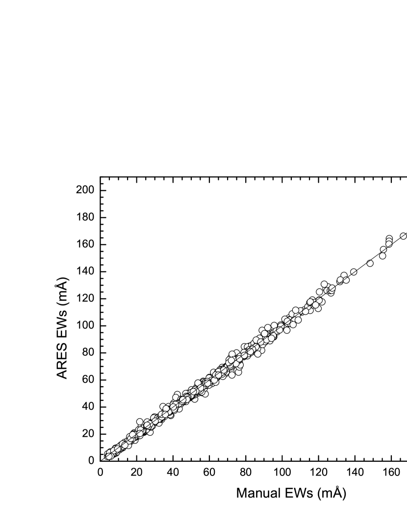
Figure 1: A comparison between manual (using IRAF splot) and automatic measurements of equivalent widths (using ARES code) for a sample of Fe I and Fe II lines in six target stars and the Sun. The solid line represents perfect agreement.

The exercise above indicates that the equivalent widths which were measured automatically using the ARES code are consistent with our measurements, although there is a slight trend of ARES equivalent widths being marginally smaller than the ones measured manually in this study. This result is in line with what was found in Sousa et al. (2007). Although we find an overall good agreement between manual and automatic equivalent widths, it is important to carefully check the results because ARES does not make quality assessments of the measurements it outputs. For instance, in the tests decribed above we note that there were 10 lines with obviously erroneous equivalent width measurements, which were discarded. In this study we estimate an uncertainty of $\sim$2 mÅ as the typical uncertainty in the equivalent width measurements. Differences in equivalent widths of $\pm$ 2 mÅ are about what is expected given the resolution, sampling, and S/N of the spectra and no significant systematic effects are found between ARES and manual measurements.

3.3 Derivation of Stellar Parameters and Iron Abundances

Stellar parameters (T_eff, $\log g$ and $\xi$) and metallicities ([Fe/H]) were derived homogeneously and following standard spectroscopic methods which are based on requirements of excitation and ionization equilibria. This abundance analysis was done in Local Thermodynamic Equilibrium (LTE) using the 2002 version of MOOG (Sneden 1973). In all calculations van der Waals constants were multiplied by an enhancement factor of 2.0 (Holweger et al. 1991). The model atmospheres in this study were interpolated from the ODFNEW grid of ATLAS9 models (Castelli & Kurucz 2004).

Effective temperatures and microturbulent velocities were iterated until the slopes of A(Fe I) versus excitation potential, $\chi$, and A(Fe I) versus reduced equivalent width,$\log(EW/\lambda)$, were respectively zero (excitation equilibrium). Only lines with $\log(EW/\lambda)<-5.00$ (this limit was changed to larger values for cooler stars) were used in the first iteration, in order to decouple the T_eff and $\xi$ determinations. Surface gravities were iterated until Fe I and Fe II returned the same mean abundances (ionization equilibrium). At the end of the iterative process, a consistent set of values of T_eff, log g and microturbulent velocity as well as the mean Fe I (= Fe II) abundance is obtained for the star. This procedure was adopted for all stars in our sample except for seven targets which had lower metallicities and solar temperatures (namely HD 6434, HD 51929, HD 80913, HD 114762, HD 153075, HD 155918 and HD 199288). In these cases, the microturbulent velocities were kept at a fixed value because there were no lines strong enough in order to anchor the iteration of this parameter. As an example, Figure 2 shows the final iterated plots of A(Fe I) versus $\chi$ (top panel) and A(Fe I) versus $\log(EW/\lambda)$ (bottom panel) for target HD 2039.

Figure 2: The spectroscopic determination of effective temperature and microturbulent velocity for HD 2039 obtained from zero slopes in the runs of Fe I abundances with excitation potential of the transitions (top panel) and reduced equivalent widths (bottom panel). The solid line represents the mean iron abundance and the dashed lines represent the 1-$\sigma$ of the distribution. The top panel shows only those lines with $\log(EW/\lambda)<-5.00$ which were used in the T_eff iteration. Fe I and Fe II abundances are consistent and the slopes are zero for A(Fe) = 7.73.

An Automated Analysis: Due to the large number of stars in our sample and Fe lines included in the analysis, BASH and FORTRAN codes were built in order to automate the whole iterative process described above. In summary, the code starts with automatic equivalent width measurements using ARES (Section 3.2) and iterates to a final set of consistent values of effective temperature, surface gravity, microturbulence and Fe abundance (both from Fe I and Fe II). With the development of an automatic procedure it is now possible to analyze the entire sample of over 300 stars studied here in a few days without interventions.

In order to further test our line list (Table 2) and analysis method, the solar spectrum (observed with FEROS spectrograph on August 20, 2008) was analyzed in a similar manner, with automatic measurements of equivalent widths (the measured solar equivalent widths are found in the last column of Table 2). Solar abundances A(Fe I) = 7.43 $\pm$ 0.07 and A(Fe II) = 7.44 $\pm$ 0.05 as well as a microturbulence $\xi$ = 1.00 km $\rm s^{-1}$ were derived using a Kurucz ODFNEW model atmosphere with $T_{\rm eff}$ = 5777 K, $\log g$ = 4.44, a model turbulence of $\xi$ = 2.0 km $\rm s^{-1}$, and l/H_p = 1.25. This solar Fe abundance is in excellent agreement with the results of Reddy et al. (2003) and Fulbright et al. (2006) (A(Fe)=7.45), which use gf-values from the same sources as here. The derived solar iron abundance also compares well (within the uncertainties) with recent solar abundance determinations for 3D hydrodynamical models from Asplund et al. (2009, A(Fe)= 7.50 $\pm$ 0.04) and Caffau et al. (2010, A(Fe)=7.52 $\pm$ 0.06).

Final values of effective temperatures, surface gravities and microturbuleny velocities for all stars are presented in Table 3. The metallicities [Fe/H] (listed in the last column in Table 3) were calculated for a solar abundance A(Fe)_☉ = 7.43 (as derived here). The $\sigma$-values listed in columns 6 and 8 correspond to the standard deviations of the final mean abundances of Fe I and Fe II. The number of Fe I and Fe II lines considered for each star are listed in columns 7 and 9, respectively.

As a comparison, photometric effective temperatures were also derived using the T_eff versus $V-K$ calibration recently published by Casagrande et al. (2010). The $V$ and $K_{s}$ magnitudes for the target stars were taken, respectively, from The Hipparcos and Tycho Catalogues (ESA 1997) and the 2MASS All-Sky Catalog of Point Sources (Cutri et al. 2003). A comparison between the spectroscopic and photometric temperatures shows that the latter are systematically higher (Figure 3). The mean difference for all studied stars is $\Delta T_{eff}(spec-phot)=-63\pm 113$ K, indicating reasonable agreement.

Uncertainties in the parameters $T_{\rm eff}$, log g, $\xi$ and [Fe/H] were estimated as in Gonzalez & Vanture (1998) and can be seen in Table 3. We note that these are internal errors and that the real uncertainties might be somewhat larger. Departures from LTE were not considered in this study and these can affect the derived LTE abundances. Non-LTE effects are expected to be smaller for Fe II lines as Fe II (and not Fe I) is the dominant ionization stage in solar type stars. For Fe I, departures from LTE are larger and may be at the level of $\sim$0.1 dex (Gehren et al. 2001a, b).

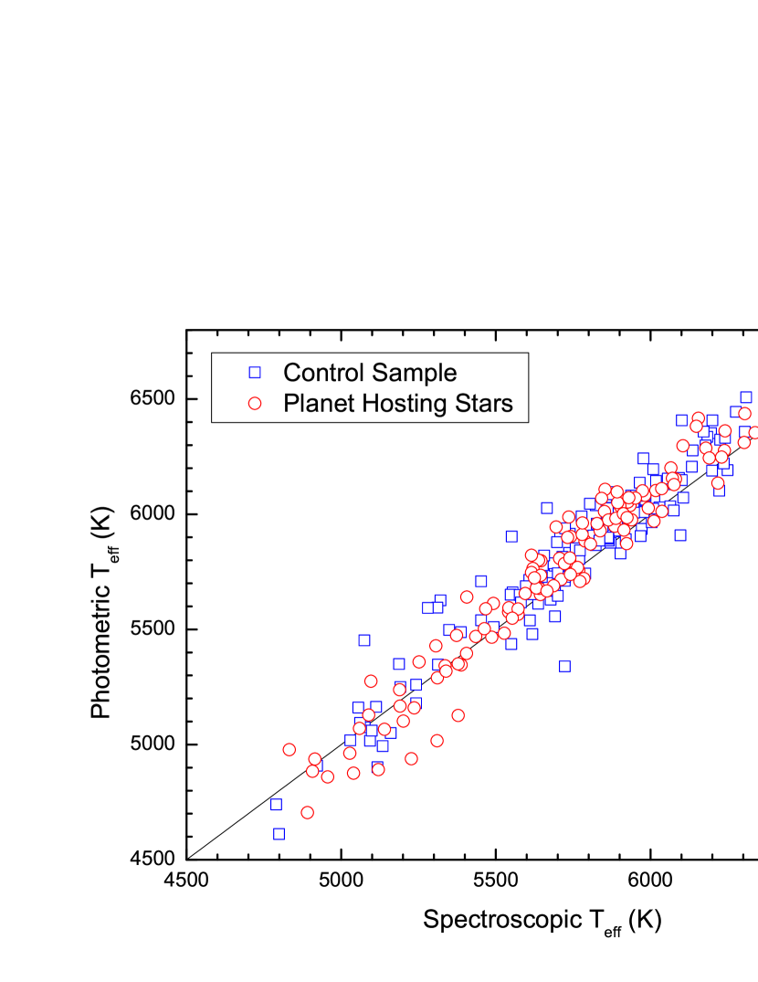
Figure 3: A comparison between photometric temperatures derived with the $V-K$ calibration in Casagrande et al. (2010) and spectroscopic temperatures derived in this study for planet hosting stars (red open circles) and control sample (blue open squares). The solid line represents the bisector. The two effective temperature scales are in reasonable agreement, however, there is a tendency for the photometric $T_{eff}$s to be higher than the spectroscopic ones at the high $T_{eff}$ end and lower at the low $T_{eff}$ end.

3.4 Evolutionary Parameters

Stellar luminosities, masses, radii and ages define the evolutionary stages of stars and for this sample these were calculated in the following way. Absolute magnitudes $M_{V}$ were determined using the classical formula:

$$M_{V}=V+5+5\log\pi-A_{V}.$$ (1)

As already mentioned, the apparent $V$ magnitudes (Table 1) were taken from The Hipparcos and Tycho Catalogues (ESA 1997). As the uncertainties in this magnitude are not listed, we adopted the errors in $V_{T}$, given the similarities between the two passbands (van Leeuwen et al. 1997). The parallaxes $\pi$ and their uncertainties (Table 4; columns 2 and 3) were taken from van Leeuwen (2007). Three stars (namely HD 70573, BD-10 3166 and WASP 2) were not present in the sources above, thus their $V$ magnitudes and parallaxes come from the references in SIMBAD and The Extrasolar Planet Encyclopaedia. The interstellar monochromatic extinction at $V$ magnitude, $A_{V}$ (Table 4; column 4), as well as its error were calculated using the tables from Arenou et al. (1992) and the code EXTINCT.FOR from Hakkila et al. (1997). Note that the Arenou et al. (1992) model is accurate to distances within 1 kpc of the Sun.

Absolute magnitudes were converted to bolometric magnitudes $M_{bol}$ by adding bolometric corrections in the $V$ band, $BC_{V}$ (Table 4; column 5), linearly interpolated from the grids of Girardi et al. (2002) for the atmospheric parameters given in Table 3. The luminosities were then calculated using the well known relation:

$$\log\frac{L}{L_{\sun}}=-0.4(M_{bol}-M_{bol,\sun}),$$ (2)

where $M_{bol,\sun}=4.77$ (Girardi et al. 2002). The uncertainties in $M_{V}$, $M_{bol}$ and $\log(L/L_{\sun})$ were derived considering that $\sigma(BC_{V})$ and $\sigma(M_{bol,\sun})$ are zero. The luminosities and uncertainties are listed in Table 4 (columns 6 and 7).

Effective temperatures and luminosities were used to place the stars on a grid of Y² isochrones from Demarque et al. (2004), thus allowing for an age determination. An interpolation code provided by the authors was used in order to obtain a set of isochrones ranging from 1.0 to 13.0 Gyr in age and from $-$0.70 dex to +0.40 dex in metallicity (with steps of 1.0 Gyr and 0.1 dex, respectively). As an example, we show the grid of isochrones for [Fe/H] = +0.30 dex in Figure 4 (top panel). The locations of all targets stars are indicated. The age of the closest isochrone was attributed for each star. Given the uncertainties in T_eff, $\log(L/L_{\sun})$ and [Fe/H] and the proximity of the isochrones, an age interval was also estimated for each star together with a single age (see Table 4). Also, some stars were located outside the grid and their ages were indicated as lower or upper limits.

Stellar radii and spectroscopic masses M_spec (as well as their uncertainties) were derived using standard relations (see e.g. eqs. 5-8 from Valenti & Fischer 2005). The masses were also calculated by placing the stars on a grid of evolutionary tracks from Yi et al. (2003). The mass of the closest track was attributed for each star. An interpolation code (provided by the authors) was used in order to obtain a set of tracks ranging from 0.5 to 2.0 $M_{\sun}$ in mass and from $-$0.70 dex to +0.40 dex in metallicity (with steps of 0.1 $M_{\sun}$ and 0.1 dex, respectively). A typical uncertainty in mass of 0.1 $M_{\sun}$ was estimated by considering the errors in T_eff, $\log(L/L_{\sun})$ and [Fe/H]. In some cases, however, this error was larger because of the location of the star on the grid or due to a larger uncertainty in the luminosity. Also, a few stars were located below the Zero Age Main Sequence (ZAMS) and their masses had to be estimated through an extrapolation. As an example, the grid of evolutionary tracks for [Fe/H] = +0.30 dex is shown in Figure 4 (bottom panel). The stellar radii and masses (spectroscopic, M_spec, and those derived with the evolutionary tracks, M_track) can be found in Table 4.

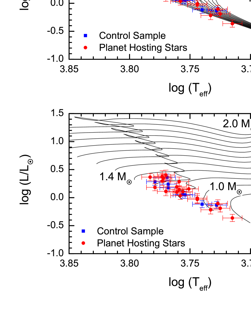
Figure 4: The location of sample planet hosting stars (red circles) and control disk sample stars (blue squares) in an HR diagram. The values of effective temperature and luminosity for the targets are from Tables 3 and 4, respectively. The top panel shows isochrones for ages varying between 1 and 13 Gyr and the bottom panel shows evolutionary tracks for mass tracks between 0.8 and 2 $M_{\sun}$. The grids of isochrones and evolutionary tracks were calculated for [Fe/H] = +0.30 dex (Demarque et al. 2004; Yi et al. 2003)

As the spectroscopic masses have greater errors, we adopt the masses obtained with the grid of evolutionary tracks. Using those masses, the Hipparcos surface gravities can be calculated with the relation:

$$\log g=\log{g_{\sun}}+\log\frac{M}{M_{\sun}}-\log\frac{L}{L_{\sun}}+4\log\frac{T_{\rm eff}}{T_{\rm eff,\sun}},$$ (3)

where T_eff,☉ = 5777 K and $\log g_{\sun}$ = 4.44. The uncertainty in these gravities was calculated considering $\sigma(T_{eff,\sun})=0$ and $\sigma(\log g_{\sun})=0$. The results are presented in Table 4 (columns 14 and 15). In Figure 5 we show a comparison between the derived spectroscopic log g’s (listed in Table 3) with Hipparcos log g’s (listed in Table 4; column 14). The line indicating perfect agreement is also shown as a solid line in the figure. The agreement between the two sets of log g’s is good although we note that the Hipparcos gravities are typically found to be higher (by 0.06 dex on the average) than the spectroscopic values with a standard deviation of $\pm$0.15 dex, which is of the order of the estimated uncertainties in the derived log g from the iron line analysis.

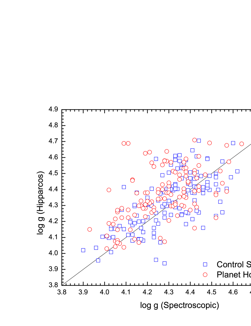
Figure 5: A comparison between Hipparcos and spectroscopic gravities for planet hosting stars and control sample. The agreement between the two sets of surface gravities is found to be good and systematic differences between the two independent scales are less than $\sim$ 0.1 dex on average. The solid line is the bisector and represents the perfect agreement between the two determinations.

In addition, masses, radii, ages and trigonometric gravities were also derived with Leo Girardi’s web code PARAM, which is based on a Bayesian parameter estimation method (da Silva et al. 2006). The mean differences between the results discussed above (This work - Girardi’s code) are small and indicate good agreement: $\Delta M=0.03\pm 0.05M_{\sun}$ (N=262), $\Delta R=0.01\pm 0.06R_{\sun}$ (N=223), $\Delta t=0.37\pm 1.46$ Gyr (N=211) and $\Delta\log g=0.03\pm 0.05$ (N=262).

4 Discussion

4.1 Comparisons with Other Studies

Several recent studies in the literature have derived stellar parameters and metallicities for samples of planet hosting stars. In the following we briefly summarize some of these works and then compare their results of effective temperatures, surface gravities and metallicities with the ones obtained in this study.

Laws et al. (2003) determined spectroscopic parameters for 30 stars with giant planets and/or brown dwarf companions. Their analysis method is similar to this study, the difference being the line list and gf-values which were obtained from an inverted solar analysis. Santos et al. (2004, 2005) did a spectroscopic analysis of a large sample of stars with and without planets (119 and 94 targets, respectively). Their method is very similar to the one used by Laws et al. (2003), with the difference being the list of iron lines (the gf-values are also solar). Takeda et al. (2005) obtained stellar parameters for a set of 160 mid-F through early-K dwarfs/subgiants. The difference with previous studies is the selected iron lines. Valenti & Fischer (2005) derived stellar properties for 1040 nearby F, G and K stars observed as part of the Keck Observatory, Lick Observatory and Anglo-Australian Telescope (AAT) planet search programs. Their method was different; stellar parameters and abundances were determined from a direct comparison of observed and synthetic spectra across certain spectral intervals using the spectral modelling program, SME. In addition, a fixed value of 0.85 km $\rm s^{-1}$ for the microturbulence was adopted for all stars. Luck & Heiter (2006) derived atmospheric parameters for a sample of 216 nearby dwarf stars. They used the standard spectroscopic method, but with differential abundances relative to the Sun. Bond et al. (2006) determined atmospheric parameters from 136 G-type stars from the AAT planet search program. In that study, photometric temperatures are obtained from $\bv$ colours listed in the Hipparcos catalog, with discrete values of microturbulence set at 1.00, 1.25 and 1.50 km $\rm s^{-1}$. The metallicities and gravities are determined by iterating this parameters until the Fe I and Fe II abundances are the same. Sousa et al. (2008) derived spectroscopic parameters for all 451 solar-type stars from the HARPS Guaranteed Time Observations (GTO) “high-precision” sample. Their method closely resembles that from Santos et al. (2004, 2005), except for a larger line list and the usage of automatic measurements of equivalent widths.

A direct comparison of the stellar parameters and metallicities obtained for some studied stars in our sample with results from other studies discussed above is possible given that there are several targets in common. Table 5 shows the average differences (in the sense This study - Literature study) computed for the effective temperatures ($\langle\Delta T_{eff}\rangle$), surface gravities ($\langle\Delta\log g\rangle$) and metallicities ($\langle\Delta[Fe/H]\rangle$) obtained for all target stars we have in common with the studies of Laws et al. (2003); Santos et al. (2004, 2005); Takeda et al. (2005); Valenti & Fischer (2005); Luck & Heiter (2006); Bond et al. (2006); Sousa et al. (2008); Santos et al. (2004, 2005). The number of stars compared in each case is found in Table 5 (column 5). Results from this simple and direct comparison are briefly summarized below.

Effective Temperatures: In general, there is not a significant offset in the effective temperature scale in this study in comparison with the other studies in Table 5. In particular, for 5 studies we find $\langle\Delta T_{eff}\rangle$ to be less than 15 K, which is a quite small systematic offset; the Luck & Heiter (2006) study has a difference which is only slightly larger ($\sim$35 K). A comparison with the $T_{eff}$ from results in Bond et al. (2006) indicates, however, a more significant systematic difference of $\sim$75 K. The standard deviations around the mean values are all $\sim$100 K or less, which is in general agreement with the estimated uncertainties for the derived effective temperatures in this study.

Surface Gravities: A direct comparison between the average surface gravity value derived for selected targets in this study with average results from Laws et al. (2003); Santos et al. (2004, 2005); Valenti & Fischer (2005); Luck & Heiter (2006) and Sousa et al. (2008) indicates that there is a small offset ($\sim$ 0.08 dex – 0.12 dex) in the $\log g$ scales. An agreement (at the level of 0.05 dex or better) is found between our results and Takeda et al. (2005) and Bond et al. (2006). The stardard deviations of the distributions around the average differences in log g are in all cases less than 0.2 dex; in agreement with the estimated uncertainties in the derived surface gravities.

Metallicities: In terms of average metallicity values, the iron abundances derived in this study compare very well with results obtained in other studies in the literature for stars in common. There is a slight tendency, however, for the metallicities here to be just marginally lower (0.03 dex or less) than the other studies; but such differences are probably statistically insignificant. Note, however, that the iron abundance results in Bond et al. (2006) are on average 0.09 dex lower than ours.

4.2 Metallicity Trends with Effective Temperature and Stellar Mass

Given our sample of 262 stars which have been subjected to a homogeneous analysis it is possible to search for differences in the properties of stars with planets compared to those stars not known to harbor giant planets with periods less than about 4 years. Two key defining properties of stars are their effective temperatures and masses, which on the main-sequence are related to each other, such that increasing T_eff maps into increasing mass, at least over the relatively limited range of metallicities explored in this sample. In order to isolate possible differences between the two samples that might be related to T_eff or mass, stars having surface gravities with $\log g<$ 4.2 were excluded from comparisons in this section. The resultant sample consists of 79 stars with planets and 109 stars without planets. Figure 6 compares the properties T_eff and derived evolutionary track mass for the two samples of stars, with mass plotted versus T_eff. The main-sequence nature of these stars is obvious from the figure, with no significant differences in the distribution along the main sequence of stars with and without planets.

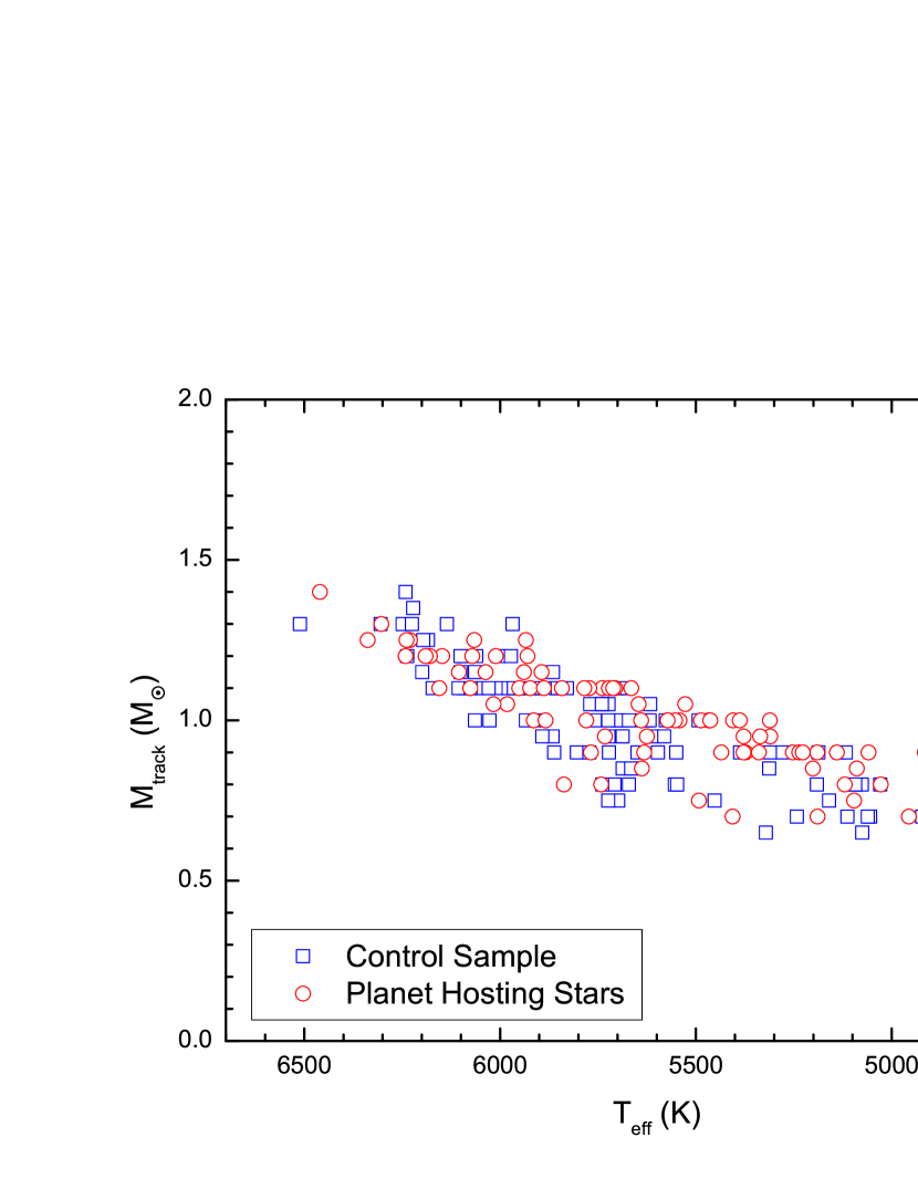
Figure 6: The relation between evolutionary track mass and effective temperatures for stars with (red open circles) and without (blue open squares) planets. Stars in both samples populate a well-defined “main-sequence”, with significant overlap in mass and T_eff between the stars with giant planets and those without.

4.2.1 Effective Temperatures, Iron Abundances and Solid-Body Accretion

The defined set of target stars with log g $\geq$ 4.2 (or those very near to the main sequence) are now illustrated with their values of [Fe/H] plotted versus T_eff in Figure 7. The top panel contains stars without planets and the bottom panel shows stars with planets. Since these are main-sequence stars, the effective temperature follows the stellar mass. No strong trends between [Fe/H] and T_eff are apparent in either sample, with the lack of an increase of [Fe/H] with increasing effective temperature placing limits on the amount of solid-body accretion (material depleted in H and He, for example) that might have occurred in these stars, since the convective-zone mass of a main-sequence star is a strongly decreasing function of increasing T_eff.

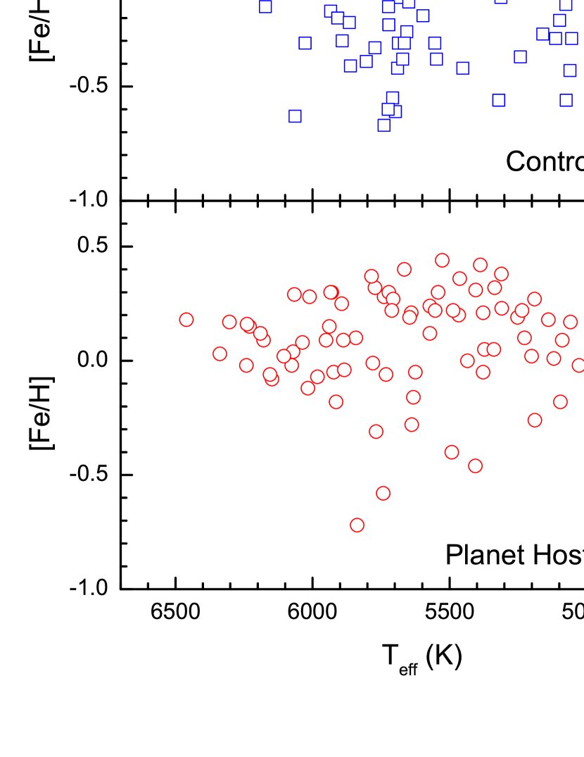
Figure 7: The trend between metallicities and effective temperatures for control sample stars (upper panel) and planet hosting stars (lower panel). There is a spread of metallicities at each T_eff, with no strong trends. Significant solid-body accretion would produce an upturn in the upper envelope of [Fe/H] with increasing T_eff: such an effect is not observed in either sample.

This same accretion test was conducted by Pinsonneault et al. (2001) on an early small sample ($\sim$30) of stars with planets and they found no trend of increasing [Fe/H] with T_eff. Accretion of solid material could create a positive trend due to the significantly decreasing convective zone mass in main-sequence stars with increasing effective tempratures: e.g., the convective-zone mass decreases by about a factor of 50 in going from T_eff = 5000 K to 6400 K (Pinsonneault et al. 2001). Accretion of only a few Earth masses of solid material would increase the surface value of [Fe/H] by $\sim$+0.3 dex in a solar-metallicity star with T_eff = 6400 K (see Figure 2 in Pinsonneault et al. 2001). No such trend is seen in Figure 7, suggesting that accretion of more than a few Earth masses of solid material is either rare, or such accreted material sinks rapidly out of the outer convection zone.

4.2.2 Stellar Mass and Metallicity

In addition to the comparison carried out above between [Fe/H] and T_eff, it is also instructive to do a similar comparison with stellar mass (in this case using the evolutionary track masses); this comparison is shown in Figure 8, again, where stars without planets are plotted in the upper panel and stars with planets in the lower panel. The samples have been binned in mass intervals of 0.25 M_☉, as represented by the error bars in the abscissa. The values of [Fe/H] plotted represent the mean value within that mass interval, with the error bars showing the standard deviations of [Fe/H] at that mass. In both samples, the values of [Fe/H] increase with increasing stellar mass. Such an increase was noted in the review by Gonzalez (2006, his Figure 1) using the abundance results from Fischer & Valenti (2005).

A signature of solid-body accretion polluting the stellar convective envelopes would be an upturn in [Fe/H] with increasing stellar mass, since the convective envelope mass is a rapidly decreasing function of increasing stellar mass. At first glance, the increase in [Fe/H] with mass found here (and noted by Gonzalez 2006 based on the Fischer & Valenti 2005 results) might suggest that solid-body accretion has taken place. Two effects, however, indicate that this has not affected the overall metallicities. First, the slopes of $\Delta$[Fe/H]/$\Delta$M are identical in both the stars with planets and stars without planets. This slope is very roughly +0.7 dex/M_☉ and is similar to the slope that would be deduced from Figure 1 in Gonzalez (2006). The fact that all of the various samples of stars, with and without giant planets, exhibit similar behavior in metallicity with mass argues that pollution has not selectively altered the values of [Fe/H] in a significant way for the stars with giant planets. The second point to note is that a positive slope of [Fe/H] with stellar mass would result from an age-metallicity relation. Since more massive stars have shorter main-sequence lifetimes, they would be biased towards higher values of [Fe/H], while lower-mass stars would be a mixture of old and young stars, which would shift the overall distribution to lower average values of [Fe/H].

In summary, comparisons among iron abundances with effective temperatures and stellar masses in both samples of stars (with and without large planets, respectively) reveal that accretion of solid-body material does not affect significantly ($\sim$0.1-0.2 dex) the overall bulk metallicity in either sample. This does not rule out smaller amounts of accretion, which might affect abundance ratios between certain types of elements (such as volatile versus refractory species, as suggested by Smith et al. 2001; see Meléndez et al. 2009 for an alternative interpretation). This question will be addressed in a later paper using the spectra from this dataset and analyzing a broad range of elements.

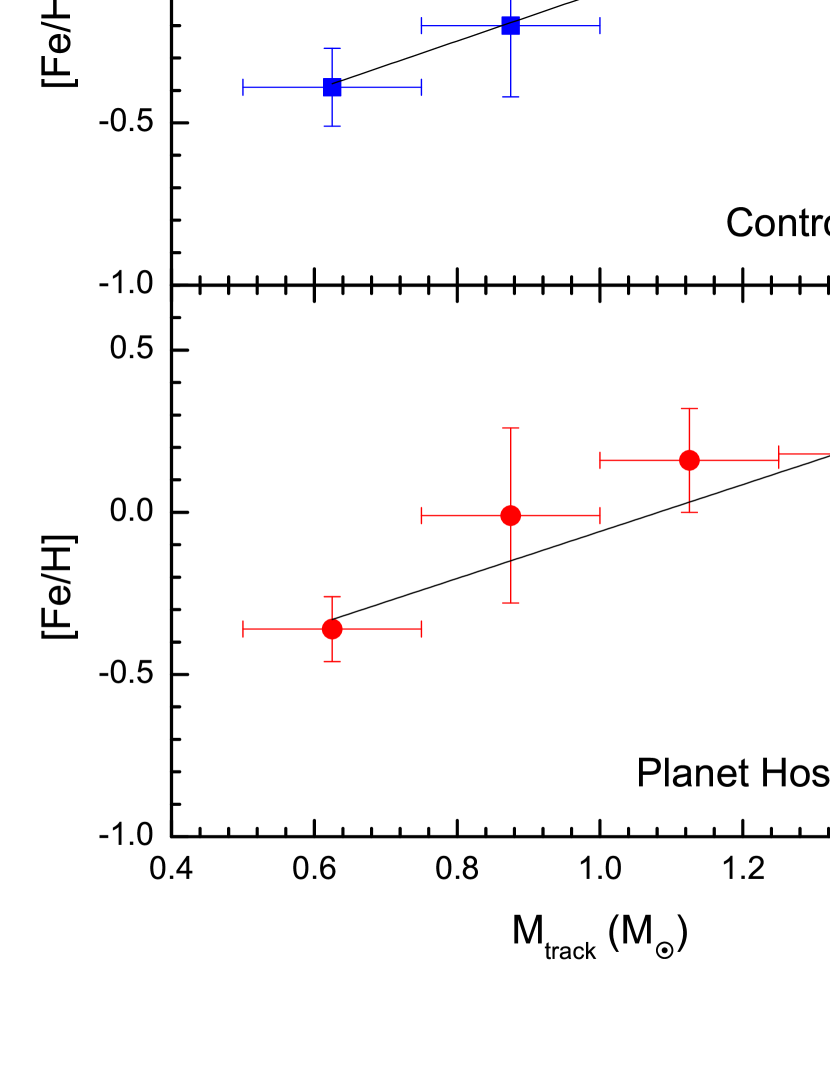
Figure 8: Average metallicities versus binned evolutionary track mass for control sample stars (upper panel) and planet hosting stars (lower panel). Masses are binned in 0.25 M_☉ intervals with each point showing the mean value and standard deviation of [Fe/H] within that mass interval. The slopes of $\Delta$[Fe/H]/$\Delta$M are the same within their uncertainties, in each sample and are likely the result of the age-metallicity relation. Selective accretion of solid-body material in stars with giant, closely orbiting planets would result in different slopes between the two samples and this is not observed.

4.3 Metallicity Distributions of Sample Stars

As discussed in Section 4.1 the metallicities ([Fe/H]) derived here are generally consistent (within the expected errors) with metallicities found in other studies of planet hosting stars in the literature. As the present study relies on a homogeneous and self-consistent analysis of a sample of 262 stars, having comparable numbers of planet hosting and comparison disk stars, it is possible to quantify differences in the metallicity distributions in these two populations. Figure 9 shows the metallicity distributions for stars with planets (solid line histogram) and comparison stars (dashed line histogram). There is an offset in the peak metallicity of the two histograms in the figure. The peak of the distrbution for stars with planets is located in the bin centered at [Fe/H] = +0.20 dex and the average metallicity of this sample is $\langle[Fe/H]\rangle$ = +0.11 dex. For the comparison stars, the peak is on the bin centered at [Fe/H] = +0.10 dex and the average metallicity in this case is lower: $\langle[Fe/H]\rangle=-0.04$ dex. Thus, there is an offset of 0.15 dex between the mean metallicities of the two samples.

When comparing properties, such as metallicity, between samples of planet hosting stars and those without giant planets, it is worth noting some selection biases inherent in these samples. As summarized by Gonzalez (2006), Doppler surveys avoid young, chromospherically active stars (which also typically are fast rotators) and contain only small numbers of metal poor stars (with [Fe/H] $<$ -0.5 dex) because these objects are rare in the solar neighbourhood. In particular, our control sample of disk stars would also suffer from such biases since it was selected in order to search for the presence of planets.

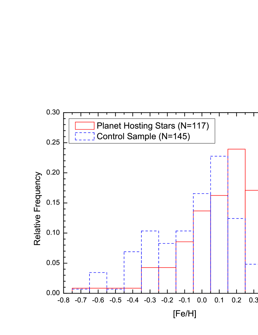
Figure 9: Metallicity distributions obtained for planet hosting stars (red solid line) and a control sample of disk stars not known to host giant planets (blue dashed line). The peaks of the metallicity distributions are offset by 0.15 dex indicating that the sample of stars which host planets is typically more metal rich.

As this offset between the peak values of the two histograms is of the order of, or just slightly higher than, the expected uncertainties in the derived iron abundances themselves, it is useful to perform a robust statistical test in order to further investigate whether the metallicity offset is meaningful. In this sense, we conducted a Two-Sample Kolmogorov-Smirnov test and found a probability $P=6.17\times 10^{-6}$ that the two samples are drawn from the same parent population. This low probability confirms the results previously found in the literature that the population of stars hosting giant planets is more metal-rich than the population of stars not known to harbour such planets.

If a volume limited sample with a radius of 18 pc is defined here for comparison, the mean metallicity for the control sample disk stars (N=46) is now -0.11 dex and the offset relative to planet-hosting stars becomes 0.22 dex, similar to the one found by Fischer & Valenti (2005) based on a much larger sample. The average metallicity found for the volume-limited sample in this study is also consistent with the results from Santos et al. (2004, 2005) and Sousa et al. (2008). The former study uses a comparison sample of 94 stars within 20 pc of the Sun and finds $\langle[Fe/H]\rangle=-0.11$ dex. The latter work extends the comparison sample to 385 stars and the enclosed radius to 56 pc and finds $\langle[Fe/H]\rangle=-0.12$ dex.

The results from Sections 4.2.1 and 4.2.2 indicate that solid body accretion has probably not altered surface values of [Fe/H] at the level of the offset in metallicity; the difference in [Fe/H] between the two samples suggests that intrinsic metallicity influences giant planet formation and migration.

4.3.1 Metallicities of stars hosting Neptunian-mass planets

The conclusions from the previous section favor the premise that metallicity plays a role in influencing the formation of giant planets, i.e., planets with roughly the mass of Jupiter. Within this model it is worthwhile exploring whether stellar metallicity also plays a role in the mass distribution of planetary systems. Such a comparison begins to probe how the underlying planetary system architecture might depend on metallicity. In this section, the metallicities of stars harboring only lower mass planets, i.e. those having Neptunian masses, are compared to systems containing the larger Jovian mass planets.

Sousa et al. (2008) presented preliminary results in which they found possible metallicity differences between stars hosting Jovian mass planets compared to those hosting Neptunian-mass planets ($M_{p}\sin i<25M_{\earth}$). The differences between the two metallicity distributions defined respectively by stars with Jovian-mass planets as opposed to Neptunian-mass planets indicated that these groups are not likely to belong to the same populations of stars. This conclusion, however, was based on a comparison of 63 Jovian hosting stars with a sample of 11 Neptunian hosting stars (those which contained at least one Neptune mass planet). Five of these 11 stars were M dwarfs and their metallicities were taken from the literature, while three were FG dwarfs analyzed by Sousa et al. (2008, HARPS GTO). The difference between the two metallicitiy distributions was a small mean offset of about 0.1 dex, with the Neptune hosting stars having a slightly lower mean metallicity.

Because M dwarfs are more difficult to analyze spectroscopically, due to considerable line blending and blanketing from molecules, it is necessary to consider abundance uncertainties and systematics when using results from these complex stellar spectra. Recent abundance analyses of M dwarfs include Bonfils et al. (2005); Woolf & Wallerstein (2006); Bean et al. (2006) and Johnson & Apps (2009). The studies by Bonfils et al. (2005) and Johnson & Apps (2009) point, for instance, to potentially large uncertainties in derived M dwarf abundances. For example, Johnson & Apps (2009) find an average offset of $\sim$ 0.30 dex in [Fe/H] when their abundances are compared to the same M dwarfs from Bonfils et al. (2005, see Table 6). Such discrepancies suggest that, until results for the cooler M dwarfs are on firmer ground, it is prudent to investigate the effects of both including M dwarf metallicities in such comparisons, as well as excluding them.

The sample studied here contains 9 systems which host at least one Neptunian mass planet, none of which are M dwarfs. This is the largest sample of stars hosting Neptunian size planets analyzed homogeneously for metallicities to date and this subsample can be directly compared to the Jupiter-like planet hosting stellar sample. The strength of such a comparison rests upon the fact that all stars have been analyzed homogeneously and are within a similar range of stellar parameters, so that systematic errors are not likely to produce spurious differences in the metallicity distributions. The weakness is that the sample of Neptune-mass hosts has only a small number of stars.

Figure 10 (top panel) shows histograms representing metallicity distributions of two samples: those stars hosting at least one Jupiter-mass planet (N=112; black solid line) and stars hosting only Neptune-mass planets (N=5; represented by the dashed red line). There is a hint that stars with only Neptunian planets tend to be more metal poor compared to Jovian-planet hosting stars. The average metallicity of the Neptunian hosts is -0.08 dex, while the Jupiter host metallicity distribution has an average of +0.12 dex. If a Two-Sample Kolmogorov-Smirnov test is performed, we find a probability of 8% that the stars in the two samples belong to the same metallicity population (which agrees with Sousa et al. 2008). This is a tantalizing result that suggests that metallicity may play a role not just in the formation of giant planets, but may also influence the distribution of planetary masses within exo-solar systems. This important question needs to be answered more definitively, but this will require larger samples.

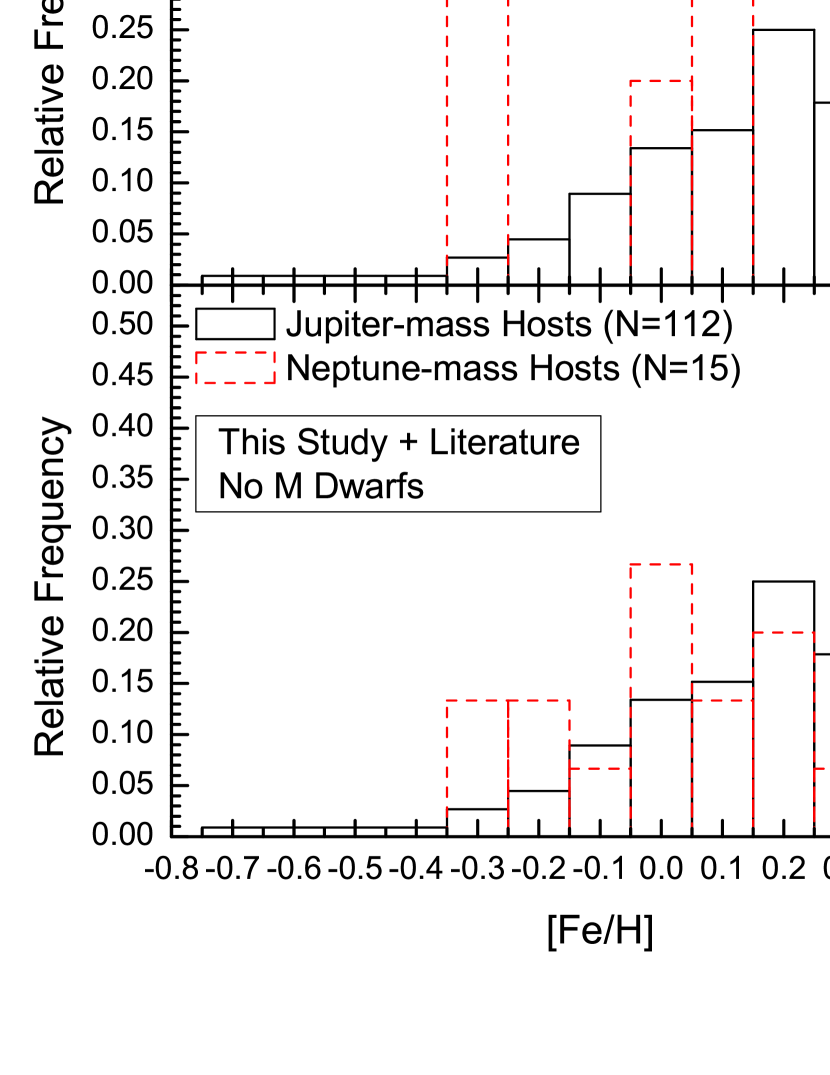
Figure 10: A comparison between the metallicity distributions for planet hosting stars. Top panel: The black solid line histogram represents the sample of planet hosting stars containing at least one Jupiter planet. The red dashed line represents the sample of stars hosting only planets with Neptune-like masses. The metallicities are from this study. Bottom panel: Results for metallicities in Neptunian-mass hosting stars from the literature are added (red dashed line histogram). Given the large uncretainties in the M dwarf metallicities these stars have not been added to the sample. There is a hint that there is offset between the two distributions represented both in the top and bottom panels.

In order to extend the sample of stars with Neptunian mass planets (shown in the top panel of Figure 10) in this discussion, a list of stars with at least one Neptunian planet was compiled from The Extrasolar Planet Encyclopaedia and is presented in Table 6 along with the metallicity results from the different studies in the literature. In a similar analysis as was done for the sample of stars studied here (discussed above), Two-Sample Kolmogorov-Smirnov tests were done now with the inclusion of the literature sample using different permutations. The results from these tests are discussed below.

1) Using the literature values of [Fe/H] for only F, G, and K dwarfs (no M dwarfs) a difference in the mean [Fe/H] of +0.11 dex (in the sense of Jovian-mass hosts minus Neptunian-mass hosts) is found, with a probability of P=17% that the two samples were drawn from the same [Fe/H] populations (with N(Jovian-mass)=112 and N(Neptunian-mass)=15). The histogram showing the comparison of these two distributions is presented in the bottom panel of 10.

2) Using all literature values, with M dwarf abundances from Johnson & Apps (2009) included, we find $\Delta$[Fe/H]=+0.10 dex and P=17% (N(Jovian-mass=112 and N(Neptunian-mass)=19).

3) When M-dwarf abundances from Bonfils et al. (2005, 2007) are used instead,$\Delta$[Fe/H]=+0.14 dex and P=5% (N(Jovian-mass)=112 and N(Neptunian-mass)=18).

In the above exercise the stars with planets were divided into systems with Jovian-mass planets and those with Neptunian-mass planets, respectively. The metallicity comparison can also be carried out by dividing the sample into stars with at least one Neptunian-mass planet, regardless of whether there is also a Jovian mass planet in the system, and those systems with Jovian mass planets but no Neptunian-mass planets. The average metallicity of the sample of stars which host at least one Neptunian planet (N=9) is +0.09 dex, close to the value derived for stars hosting at least one Jupiter-mass planet (+0.12 dex; N=112). A Two-Sample Kolmogorov-Smirnov test reveals that the probability that these two samples belong to the same parent population is 91%. This comparison strengthens the idea that metallicity played a role in setting the mass of the most massive planet in a system.

All of these various comparisons taken together suggest that lower values of [Fe/H] tend to produce lower-masses of the most massive planet within a planetary system. Such conclusions, however, should be viewed with caution since the number of stars harboring Neptune-size planets analyzed to date is still rather small, but in line with what would be expected from models of planet formation via core accretion (Ida & Lin 2004; Mordasini et al. 2009a, b; see also review by Boss 2010).

5 Conclusions

We have determined stellar parameters for 117 main-sequence stars with planets discovered via radial velocity surveys and 145 comparison stars which have been found to exhibit nearly constant radial velocities and are not likely to host large, closely orbiting planets. The stellar parameters were derived from a classical spectroscopic analysis, using accurate laboratory gf-values of Fe lines and automatically measured equivalent widths, after critical evaluations of their quality. The values of effective temperature, surface gravity (as $\log g$), microturbulent velocities, and iron abundances are in general good agreement with most of the values presented in a number of literature studies, but problems with a few individual stars may remain.

Correlations between [Fe/H] and T_eff in members of either sample are not found, which places stringent limits on the possible accretion of solid material (of less than a few Earth masses) onto the surfaces of these stars. A trend of increasing [Fe/H] with increasing stellar mass is found in both samples of stars, with the slope of $\Delta$[Fe/H]/$\Delta$M being the same for stars with giant planets and control sample stars. The same value of $\Delta$[Fe/H]/$\Delta$M for both samples rules out solid-body accretion, which leaves the underlying disk age-metallicity relation as the likely cause of the positive correlation of [Fe/H] with mass.

It should be noted that the samples analyzed here were not selected based on any rigourous criteria, other than being segregated based on the presence of giant planets in one sample and the probable absence of such planets in the other. The list of stars without planets preferentially included metal-rich stars, while some stars with planets were discovered by surveys that were based on high-metallicity as a criterion.

A comparison of iron abundances between the stars with planets with the results from the control sample of disk stars confirms the results obtained by previous studies showing that planet-hosting stars exhibit larger metallicities than stars not harboring planets; the difference found in this sample is that stars with planets are shifted by +0.15 dex in [Fe/H] when compared to the stars without planets.

The sample of stars with planets discussed here contains 9 stars which host at least one Neptunian-mass planet; of these 9 systems, 4 also contain a Jovian-mass planet, while 5 contain only Neptunian-sized planets and no Jovian-mass closely orbiting planets. A statistical test of the iron abundances indicates that there is probably a real difference between the metallicity distributions of stars which contain only smaller Neptunian-sized planets in comparison with stars hosting the larger Jovian-mass planets (see also Sousa et al. 2008).

Although it should be recognized that the sample sizes are still small, there seems to be early indications that metallicity plays an important role in setting the mass of the most massive planet. It is also important to note that such a conclusion obtained here is based on stars which have all been analyzed homogeneously and which also have similar stellar parameters, therefore avoiding the large uncertainties still hampering the analyses and derived metallicities for the cooler M dwarfs. The same statistical test applied to metallicity results in the literature obtained for all FGK stars which host only Neptunian-sized planets allows for a larger sample and overall corroborates the results obtained with our sample.

Table 1: Log of Observations

Star	$V$	Observation	$T_{exp}$	S/N
		Date	(s)	($\sim$ 6700 Å)
Planet Hosting Stars
HD 142	5.70	2007 Aug 30	200	367
HD 1237	6.59	2007 Aug 30	480	466
HD 2039	9.00	2007 Aug 28	3000	362
HD 2638	9.44	2007 Aug 29	3000	276
HD 3651	5.88	2007 Aug 29	200	356
Control Sample
HD 1581	4.23	2008 Aug 20	30	216
HD 1835	6.39	2007 Oct 02	200	388
HD 3823	5.89	2007 Oct 02	200	452
HD 4628	5.74	2008 Aug 20	200	375
HD 7199	8.06	2008 Aug 19	1200	348

Note. — Table 1 is published in its entirety in the eletronic edition of the Astrophysical Journal. A portion is show here for guidance regarding its form and content.

Table 2: Selected Fe lines and Measured Equivalent Widths for the Sun.

$\lambda$	Ion	LEP	$\log gf$	W${}_{\lambda}\sun$
(Å)		(eV)	(dex)	(mÅ)
4779.439	Fe I	3.415	$-$2.020	40.4
4788.751	Fe I	3.237	$-$1.763	63.3
4802.875	Fe I	3.695	$-$1.514	58.3
4962.572	Fe I	4.178	$-$1.182	52.7
5054.642	Fe I	3.640	$-$1.921	39.6
5247.049	Fe I	0.087	$-$4.946	65.8
5379.574	Fe I	3.694	$-$1.514	59.8
5618.631	Fe I	4.209	$-$1.276	48.4
5741.846	Fe I	4.256	$-$1.670	30.8
5775.081	Fe I	4.220	$-$1.298	57.9
5778.453	Fe I	2.588	$-$3.430	21.3
5855.076	Fe I	4.608	$-$1.478	21.4
5916.247	Fe I	2.453	$-$2.994	55.0
5956.692	Fe I	0.859	$-$4.605	51.3
6120.246	Fe I	0.915	$-$5.970	5.2
6151.617	Fe I	2.176	$-$3.299	48.7
6173.334	Fe I	2.223	$-$2.880	67.2
6200.313	Fe I	2.608	$-$2.437	72.5
6219.279	Fe I	2.198	$-$2.433	89.8
6240.645	Fe I	2.223	$-$3.170	48.0
6265.131	Fe I	2.176	$-$2.550	84.2
6380.743	Fe I	4.186	$-$1.376	51.8
6593.870	Fe I	2.433	$-$2.422	84.5
6699.141	Fe I	4.593	$-$2.101	7.7
6739.520	Fe I	1.557	$-$4.794	11.7
6750.150	Fe I	2.424	$-$2.621	73.2
6858.145	Fe I	4.607	$-$0.930	51.1
4993.358	Fe II	2.807	$-$3.670	37.6
5132.669	Fe II	2.807	$-$4.000	26.9
5284.109	Fe II	2.891	$-$3.010	62.6
5325.553	Fe II	3.221	$-$3.170	39.2
5414.073	Fe II	3.221	$-$3.620	27.6
5425.257	Fe II	3.199	$-$3.210	41.5
5991.376	Fe II	3.153	$-$3.560	30.4
6084.111	Fe II	3.199	$-$3.800	20.5
6149.258	Fe II	3.889	$-$2.720	35.0
6369.462	Fe II	2.891	$-$4.190	19.9
6416.919	Fe II	3.892	$-$2.680	38.5
6432.680	Fe II	2.891	$-$3.580	40.4

Table 3: Atmospheric Parameters.

Star	Teff	$\log$ g	$\xi$	A(Fe)	$\sigma$	N	$\sigma$	N	[Fe/H]
	(K)		(km $\rm s^{-1}$)		(Fe I)	(Fe I)	(Fe II)	(Fe II)
Planet Hosting Stars
HD 142	6338 $\pm$ 46	4.34 $\pm$ 0.14	2.27 $\pm$ 0.08	7.46	0.09	23	0.07	10	0.03 $\pm$ 0.04
HD 1237	5572 $\pm$ 40	4.58 $\pm$ 0.09	1.34 $\pm$ 0.04	7.55	0.09	27	0.05	9	0.12 $\pm$ 0.04
HD 2039	5934 $\pm$ 36	4.30 $\pm$ 0.13	1.26 $\pm$ 0.04	7.73	0.08	27	0.05	12	0.30 $\pm$ 0.03
HD 2638	5236 $\pm$ 70	4.38 $\pm$ 0.19	0.86 $\pm$ 0.04	7.65	0.07	26	0.07	9	0.22 $\pm$ 0.05
HD 3651	5252 $\pm$ 65	4.32 $\pm$ 0.18	0.81 $\pm$ 0.02	7.62	0.08	27	0.05	10	0.19 $\pm$ 0.03
Control Sample
HD 1581	5908 $\pm$ 31	4.26 $\pm$ 0.13	1.17 $\pm$ 0.04	7.23	0.08	25	0.08	12	$-$0.20 $\pm$ 0.03
HD 1835	5829 $\pm$ 41	4.39 $\pm$ 0.16	1.24 $\pm$ 0.04	7.65	0.07	22	0.05	10	0.22 $\pm$ 0.03
HD 3823	6012 $\pm$ 31	4.18 $\pm$ 0.08	1.92 $\pm$ 0.10	7.08	0.07	25	0.05	11	$-$0.35 $\pm$ 0.02
HD 4628	5055 $\pm$ 40	4.33 $\pm$ 0.19	0.88 $\pm$ 0.04	7.14	0.08	25	0.06	5	$-$0.29 $\pm$ 0.02
HD 7199	5349 $\pm$ 65	4.09 $\pm$ 0.19	1.04 $\pm$ 0.04	7.74	0.09	26	0.05	10	0.31 $\pm$ 0.05

Note. — Table 3 is published in its entirety in the eletronic edition of the Astrophysical Journal. A portion is show here for guidance regarding its form and content.

Table 4: Evolutionary Parameters.

Star	$\pi$	$\sigma_{\pi}$	$A_{V}$	$BC_{V}$	$\log(L/L_{\sun})$	$\sigma_{\log(L/L_{\sun})}$	$R$	$\sigma_{R}$	$M_{spec}$	$\sigma(M_{spec})$	Mtrack	$\sigma(M_{track})$	$\log g_{Hipp}$	$\sigma(\log g_{Hipp})$	Age	$\Delta$Age
	(mas)	(mas)					(R☉)	(R☉)	(M☉)	(M☉)	(M☉)	(M☉)			(Gyr)	(Gyr)
Planet Hosting Stars
HD 142	38.89	0.37	0.05	0.017	0.462	0.061	1.41	0.11	1.59	0.77	1.25	0.10	4.24	0.08	2.5	2.0-3.5
HD 1237	57.15	0.31	0.04	$-$0.075	$-$0.196	0.060	0.86	0.07	1.02	0.49	1.00	0.10	4.57	0.08	$<$ 1.0	0.0-3.0
HD 2039	9.75	0.95	0.11	$-$0.004	0.376	0.104	1.46	0.18	1.55	0.81	1.25	0.10	4.21	0.11	3.5	3.0-4.5
HD 2638	20.03	1.49	0.10	$-$0.159	$-$0.368	0.089	0.80	0.09	0.55	0.28	0.90	0.10	4.59	0.11	$<$ 1.0	0.0-4.0
HD 3651	90.42	0.32	0.02	$-$0.153	$-$0.287	0.060	0.87	0.07	0.57	0.28	0.90	0.10	4.51	0.08	5.0	0.0-12.0
Control Sample
HD 1581	116.46	0.16	0.01	$-$0.037	0.102	0.060	1.08	0.08	0.76	0.37	1.00	0.10	4.38	0.08	6.5	4.0-9.0
HD 1835	47.93	0.53	0.08	$-$0.025	0.033	0.061	1.02	0.08	0.93	0.45	1.10	0.10	4.47	0.08	1.0	0.0-3.5
HD 3823	40.07	0.34	0.04	$-$0.035	0.376	0.061	1.42	0.11	1.11	0.54	1.00	0.10	4.13	0.08	7.5	6.5-9.0
HD 4628	134.14	0.51	0.01	$-$0.226	$-$0.549	0.060	0.69	0.06	0.37	0.18	0.70	0.10	4.60	0.09	9.0	0.0-14.0
HD 7199	28.33	0.57	0.10	$-$0.122	$-$0.132	0.063	1.00	0.08	0.45	0.22	0.95	0.10	4.41	0.08	9.0	5.0-13.0

Note. — Table 4 is published in its entirety in the eletronic edition of the Astrophysical Journal. A portion is show here for guidance regarding its form and content.

Table 5: Comparison with other results in the literature.

Study	$\langle\Delta T_{eff}\rangle$ (K)	$\langle\Delta\log g\rangle$	$\langle\Delta$[Fe/H]$\rangle$	NStars
Laws et al. (2003)	$-5\pm$74	$-$0.10$\pm$0.15	$-$0.03$\pm$0.05	23
Santos et al. (2004, 2005)	$-2\pm$72	$-$0.08$\pm$0.13	$-$0.02$\pm$0.06	113
Takeda et al. (2005)	$-8\pm$65	$-$0.05$\pm$0.16	$-$0.03$\pm$0.07	35
Valenti & Fischer (2005)	10$\pm$65	$-$0.11$\pm$0.14	$-$0.01$\pm$0.06	223
Luck & Heiter (2006)	$-32\pm$84	$-$0.11$\pm$0.15	$-$0.02$\pm$0.07	56
Bond et al. (2006)	74$\pm$113	0.01$\pm$0.19	0.09$\pm$0.09	90
Sousa et al. (2008)	$-14\pm$61	$-$0.11$\pm$0.11	0.00$\pm$0.06	119

Note. — $\Delta$ = This study - Literature Study

Table 6: Neptunian-mass Planet Hosts

Star	$M_{P}\sin\textit{i}$	Jupiter	[Fe/H]	Reference
	($M_{\earth}$)			[Fe/H]
Results from This Work
HD 4308	12.87	no	$-$0.31
HD 16417	21.93	no	0.14
HD 40307	4.20	no	$-$0.35
HD 47186	22.78	yes	0.21
HD 69830	10.49	no	0.00
HD 125612	21.29	yes	0.25
HD 160691	10.56	yes	0.23
HD 181433	7.56	yes	0.46
HD 219828	20.98	no	0.14
Literature Results
HD 7924	9.22	no	$-0.15$	Howard et al. (2009)
HD 1461	7.60	no	0.18	Valenti & Fischer (2005)
			0.21	Luck & Heiter (2006)
			0.19	Sousa et al. (2008)
			0.19	Average
CoRoT-7	4.80	no	0.05	Léger et al. (2009)
55 Cnc	7.63	yes	0.33	Santos et al. (2004)
BD-082823	14.30	yes	$-$0.07	Hébrard et al. (2010)
HD 90156	17.48	no	$-$0.24	Encyclopaedia
61 Vir	5.09	no	0.01	Santos et al. (2004, 2005)
			0.05	Takeda et al. (2005)
			0.11	Valenti & Fischer (2005)
			$-$0.02	Sousa et al. (2008)
			0.04	Average
HD 125595	14.30	no	0.02	Encyclopaedia
HD 156668	4.16	no	$-$0.07	Mishenina et al. (2008)
Kepler-4	24.47	no	0.17	Borucki et al. (2010)
HD 179079	25.43	no	0.25	Valenti et al. (2009)
HAT-P-11	25.74	no	0.31	Bakos et al. (2010)
HD 190360	18.12	yes	0.24	Sousa et al. (2008)
HD 215497	5.40	yes	0.23	Lo Curto et al. (2010)
Literature Results for M Stars
HD 285968	8.42	no	$-$0.10	Endl et al. (2008)
			0.18	Johnson & Apps (2009)
			0.04	Average
GJ 436	22.88	no	0.02	Bonfils et al. (2005)
			$-$0.32	Bean et al. (2006)
			0.25	Johnson & Apps (2009)
			$-$0.02	Average
Gl 581	1.94	no	$-$0.25	Bonfils et al. (2005)
			$-$0.33	Bean et al. (2006)
			$-$0.10	Johnson & Apps (2009)
			$-$0.23	Average
GJ 674	11.76	no	$-$0.28	Bonfils et al. (2007)
			$-$0.11	Johnson & Apps (2009)
			$-$0.20	Average
Gliese 876	6.36	yes	$-$0.03	Bonfils et al. (2005)
			$-$0.12	Bean et al. (2006)
			0.37	Johnson & Apps (2009)
			0.07	Average

References

- Arenou et al. (1992) Arenou, F., Grenon, M., & Gómez, A. 1992, A&A, 258, 204
- Asplund et al. (2009) Asplund, M., Grevesse, N., Sauval, A. J., & Scott, P. 2009, ARA&A, 47, 481
- Bakos et al. (2010) Bakos, G. Á., et al. 2010, ApJ, 710, 1724
- Bard, Kock & Kock (1991) Bard, A., Kock, A., & Kock, M. 1991, A&A, 248, 315
- Bard & Kock (1994) Bard, A., & Kock, M. 1994, A&A, 282, 1014
- Bean et al. (2006) Bean, J. L., Benedict, G. F., Endl, M. 2006, ApJ, 653, L65
- Blackwell et al. (1986) Blackwell, D. E., Booth, A. J., Haddock, D. J., & Petford, A. D. 1986, MNRAS, 220, 549
- Blackwell et al. (1984) Blackwell, D. E., Booth, A. J., & Petford, A. D. 1984, A&A, 132, 236
- Blackwell et al. (1995) Blackwell, D. E., Lynas-Gray, A. E., & Smith, G. 1995, A&A, 296, 217
- Blackwell et al. (1982a) Blackwell, D. E., Petford, A. D., Shallis, M. J., & Simmons, G. J. 1982a, MNRAS, 199, 43
- Blackwell et al. (1982b) Blackwell, D. E., Petford, A. D., & Simmons, G. J. 1982b, MNRAS, 201, 595
- Bond et al. (2006) Bond, J. C., Tinney, C. G., Butler, R. P., Jones, H. R. A., Marcy, G. W., Penny, A. J., & Carter, B. D. 2006, MNRAS, 370, 163
- Bonfils et al. (2007) Bonfils, X., et al. 2007, A&A, 474, 293
- Bonfils et al. (2005) Bonfils, X., Delfosse, X., Udry, S., Santos, N. C., Forveille, T., Ségransan, D. 2005, A&A, 442, 635
- Borucki et al. (2010) Borucki, W. J., et al. 2010, ApJ, 713, L126
- Boss (2010) Boss, A. P. 2010, in IAU Symp. 265, Chemical Abundances in the Universe: Connecting First Stars to Planets, ed. K. Cunha, M. Spite & B. Barbuy (Cambridge:Cambridge University Press), 391
- Caffau et al. (2010) Caffau, E., Ludwig, H.-G., Steffen, M., Freytag, B., Bonifacio, P. 2010 (arXiv:1003.1190)
- Casagrande et al. (2010) Casagrande, L., Ramírez, I., Meléndez, J., Bessel, M., & Asplund, M. 2010, arXiv:astro-ph/1001.3142v1
- Castelli & Kurucz (2004) Castelli, F., & Kurucz, R. L. 2004, in Proc. IAU Symp. 210, Modelling of Stellar Atmospheres ed. N. Piskunov, et al. (Dordrecht: Kluwer), poster A20 (arXiv:astro-ph/0405087)
- Cutri et al. (2003) Cutri, R. M., et al. 2003, VizieR Online Data Catalog, II/246
- da Silva et al. (2006) da Silva, L., et al. 2006, A&A, 458, 609
- Demarque et al. (2004) Demarque, P., Woo, J.-H., Kim, Y.-C., & Yi, S. K. 2004, ApJS, 155, 667
- Endl et al. (2008) Endl, M., Cochran, W. D., Wittenmyer, R. A., & Boss, A. P. 2008, ApJ, 673, 1165
- ESA (1997) ESA 1997, The Hipparcos and Tycho Catalogues, SP 1200 (ESA)
- Fischer & Valenti (2005) Fischer, D. A., & Valenti, J. 2005, ApJ, 622, 1102
- Fuhr, Martin & Wiese (1988) Fuhr, J. R., Martin, G. A., & Wiese, W. L. 1988, J. Phys. Chem. Ref. Data 17, Suppl. 4
- Fulbright et al. (2006) Fulbright, J. P., McWilliam, A., & Rich, R. M. 2006, ApJ, 636, 821
- Gehren et al. (2001a) Gehren, T., Butler, K., Mashonkina, L., Reetz, J., & Shi, J. 2001, A&A, 366, 981
- Gehren et al. (2001b) Gehren, T., Korn, A.J., & Shi, J. 2001, A&A, 380, 645
- Ghezzi et al. (2009) Ghezzi, L., Cunha, K., Smith, V.V., Margheim, S., Schuler, S., de Araújo, F.X., & de la Reza, R. 2009, ApJ, 698, 451
- Ghezzi (2010) Ghezzi, L. 2010, Ph.D. thesis, Observatório Nacional, Rio de Janeiro
- Girardi et al. (2002) Girardi, L., Bertelli, G., Bressan, A., Chiosi, C., Groenewegen, M. A. T., Marigo, P., Salasnich, B., & Weiss, A. 2002, A&A, 391, 195
- Gonzalez (1997) Gonzalez, G. 1997, MNRAS, 285, 403
- Gonzalez (2006) Gonzalez, G. 2006, PASP, 118, 1494
- Gonzalez & Vanture (1998) Gonzalez, G., & Vanture, A. D. 1998, A&A, 339, L29
- Hakkila et al. (1997) Hakkila, J., Myers, J. M., Stidham, B. J., & Hartmann, D. H. 1997, AJ, 114, 2043
- Hébrard et al. (2010) Hébrard, G., et al. 2010, A&A, 512, A46
- Holweger et al. (1991) Holweger, H., Bard, A., Kock, A., & Kock, M. 1991, A&A, 249, 545
- Howard et al. (2009) Howard, A. W., et al. 2009, ApJ, 696, 75
- Ida & Lin (2004) Ida, S., & Lin, D. N. C. 2004, ApJ, 616, 567
- Johnson & Apps (2009) Johnson, J. A., & Apps, K. 2009, ApJ, 699, 933
- Kaufer et al. (1999) Kaufer, A., Stahl, O., Tubbesing, S., Nørregaard, P., Avila, G., Francois, P., Pasquini, L., & Pizzella, A. 1999, The Messenger, 95, 8
- Kurucz et al. (1984) Kurucz, R. L., Furelind, I., Brault, J., & Testerman, L. 1984, Solar Flux Atlas from 296 to 1300 nm (Cambridge: Harvard Univ. Press)
- Kupka et al. (1999) Kupka, F., Piskunov, N., Ryabchikova, T A., Stempels, H. C., & Weiss, W. W. 1999, A&AS, 138, 119
- Lambert et al. (1996) Lambert, D. L., Heath, J. E., Lemke, M., & Drake, J. 1996, ApJS, 103, 183
- Laws et al. (2003) Laws, C., Gonzalez, G., Walker, K. M., Tyagi, S., Dodsworth, J., Snider, K., & Suntzeff, N. B. 2003, AJ, 125, 2664
- Léger et al. (2009) Léger, A., et al. 2009, A&A, 506, 287
- Lo Curto et al. (2010) Lo Curto, G., et al. 2010, A&A, 512, A48
- Lovis & Mayor (2007) Lovis, C., & Mayor, M. 2007, A&A, 472, 657
- Luck & Heiter (2006) Luck, R. E., & Heiter, U. 2006, AJ, 131, 3069
- Marcy et al. (2005) Marcy, G. W., Butler, R. P., Vogt, S. S., Fischer, D. A., Henry, G. W., Laughlin, G., Wright, J. T., & Johnson, J. A. 2005, ApJ, 619, 570
- May et al. (1974) May, M., Richter, J., Wichelmann, J. 1974 , A&AS, 18, 405
- Mayor et al. (2009) Mayor, M., et al. 2009, A&A, 493, 639
- Meléndez et al. (2009) Meléndez J., Asplund, M., Gustafsson, B., & Yong, D. 2009, ApJ, 704, L66
- Meléndez & Barbuy (2009) Meléndez J., & Barbuy B. 2009, A&A, 497, 611
- Mishenina et al. (2008) Mishenina, T. V., Soubiran, C., Bienaymé, O., Korotin, S. A., Belik, S. I., Usenko, I. A., & Kovtyukh, V. V. 2008, A&A, 489, 923
- Mordasini et al. (2009a) Mordasini, C., Alibert, Y., & Benz, W. 2009, A&A, 501, 1139
- Mordasini et al. (2009b) Mordasini, C., Alibert, Y., Benz, W., & Naef, D. 2009, A&A, 501, 1161
- O’Brian et al. (1991) O’Brian, T. R., Wickliffe, M. E., Lawler, J. E., Whaling, W., Brault J. W., 1991, J. Opt. Soc. Am. B, 8, 1185
- Pasquini et al. (2007) Pasquini, L., Döllinger, M. P., Weiss, A., Girardi, L., Chavero, C., Hatzes, A. P., da Silva, L., Setiawan, J. 2007, A&A, 473, 979
- Perryman et al. (1997) Perryman, M. A. C., et al. 1997, A&A, 323, L49
- Pinsonneault et al. (2001) Pinsonneault, M. H., DePoy, D. L., & Coffee, M. 2001, ApJ, 556, L59
- Raassen & Uylings (1998) Raassen, A. J. J., & Uylings, P. H. M. 1998, A&A, 340, 300
- Reddy et al. (2003) Reddy, B. E., Tomkin, J., Lambert, D. L., & Allende Prieto, C. 2003, MNRAS, 340, 304
- Santos et al. (2001) Santos, N. C., Israelian, G., & Mayor, M. 2001, A&A, 373, 1019
- Santos et al. (2004) Santos, N. C., Israelian, G., & Mayor, M. 2005, A&A, 415, 1153
- Santos et al. (2005) Santos, N. C., Israelian, G., Mayor, M., Bento, J. P., Almeida, P. C., Sousa, S. G., & Ecuvillon, A. 2005, A&A, 437, 1127
- Smith et al. (2001) Smith, V. V., Cunha, K., Lazzaro, D. 2001, AJ, 121, 3207
- Sneden (1973) Sneden, C. 1973, PhD thesis, Univ. Texas, Austin
- Sousa et al. (2007) Sousa, S. G., Santos, N. C., Israelian, G., Mayor, M., & Monteiro, M. J. P. F. G. 2008, A&A, 469, 783
- Sousa et al. (2008) Sousa, S. G., Santos, N. C., Mayor, M., Udry, S., Casagrande, L., Israelian, G., Pepe, F., Queloz, D., & Monteiro, M. J. P. F. G. 2008, A&A, 487, 373
- Takeda et al. (2005) Takeda, Y., Ohkubo, M., Sato, B., Kambe, E., Sadakane, K. 2005, PASJ, 57, 27
- Udry & Santos (2007) Udry, S., & Santos, N. C., 2007, ARA&A, 45, 397
- Udry et al. (2006) Udry, S., et al. 2006, A&A, 447, 361
- Valenti et al. (2009) Valenti, J. A., et al. 2009, ApJ, 702, 989
- Valenti & Fischer (2005) Valenti, J. A., & Fischer, D. A. 2005, ApJS, 159, 141
- van Leeuwen (2007) van Leeuwen, F. 2007, Ap&SSLibrary, Vol. 350, Hipparcos, the New Reduction of the Raw Data
- van Leeuwen et al. (1997) van Leeuwen, F., Evans, D. W., Grenon, M., Großmann, V., Mignard, F., & Perrymann, M. A. C. 1997, A&A, 323, L61
- Woolf & Wallerstein (2006) Woolf, V. M., & Wallerstein, G. 2006, PASP, 118, 218
- Yi et al. (2003) Yi, S. K., Kim, Y.-C., & Demarque, P. 2003, ApJS, 144, 259