XML Reconstruction View Selection in XML Databases:
Complexity Analysis and Approximation Scheme

Abstract

Query evaluation in an XML database requires reconstructing XML subtrees rooted at nodes found by an XML query. Since XML subtree reconstruction can be expensive, one approach to improve query response time is to use reconstruction views - materialized XML subtrees of an XML document, whose nodes are frequently accessed by XML queries. For this approach to be efficient, the principal requirement is a framework for view selection. In this work, we are the first to formalize and study the problem of XML reconstruction view selection. The input is a tree $T$, in which every node $i$ has a size $c_{i}$ and profit $p_{i}$, and the size limitation $C$. The target is to find a subset of subtrees rooted at nodes $i_{1},\cdots,i_{k}$ respectively such that $c_{i_{1}}+\cdots+c_{i_{k}}\leq C$, and $p_{i_{1}}+\cdots+p_{i_{k}}$ is maximal. Furthermore, there is no overlap between any two subtrees selected in the solution. We prove that this problem is NP-hard and present a fully polynomial-time approximation scheme (FPTAS) as a solution.

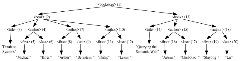
(a) XML tree

redge
ID	parentID	name	content
1	NULL	bookstore	NULL
2	1	book	NULL
3	2	title	Database Systems
4	2	author	NULL
5	4	first	Michael
6	4	last	Kifer
7	2	author	NULL
8	7	first	Arthur
9	7	last	Bernstein
10	2	author	NULL
11	10	first	Philip
12	10	last	Lewis
13	1	book	NULL
14	13	title	Querying the Semantic Web
…	…	…	…

(b) Edge table

<book>
	<title> Database Systems </title>
	<author>
		<first> Michael </first>
		<last> Kifer </last>
	</author>
	<author>
		<first> Arthur </first>
		<last> Bernstein </last>
	</author>
	<author>
		<first> Philip </first>
		<last> Lewis </last>
	</author>
</book>

(c) XML reconstruction view

Figure 1: An example of an XML tree, its relational storage, and XML reconstruction view

1 Introduction

With XML [1] being the de facto standard for business and Web data representation and exchange, storage and querying of large XML data collections is recognized as an important and challenging research problem. A number of XML databases [14, 28, 6, 22, 8, 4, 7, 2, 27, 19, 18] have been developed to serve as a solution to this problem. While XML databases can employ various storage models, such as relational model or native XML tree model, they support standard XML query languages, called XPath and XQuery. In general, an XML query specifies which nodes in an XML tree need to be retrieved. Once an XML tree is stored into an XML database, a query over this tree usually requires two steps: (1) finding the specified nodes, if any, in the XML tree and (2) reconstructing and returning XML subtrees rooted at found nodes as a query result. The second step is called XML subtree reconstruction [9, 10] and may have a significant impact on query response time. One approach to minimize XML subtree reconstruction time is to cache XML subtrees rooted at frequently accessed nodes as illustrated in the following example.

Consider an XML tree in Figure 1(a) that describes a sample bookstore inventory. The tree nodes correspond to XML elements, e.g., bookstore and book, and data values, e.g., “Arthur” and “Bernstein”, and the edges represent parent-child relationships among nodes, e.g., all the book elements are children of bookstore. In addition, each element node is assigned a unique identifier that is shown next to the node in the figure. As an example, in Figure 1(b), we show how this XML tree can be stored into a single table in an RDBMS using the edge approach [14]. The edge table $r_{edge}$ stores each XML element as a separate tuple that includes the element ID, ID of its parent, element name, and element data content. A sample query over this XML tree that retrieves books with title “Database Systems” can be expressed in XPath as:

/bookstore/book[title="Database Systems"]

This query can be translated into relational algebra or SQL over the edge table to retrieve IDs of the book elements that satisfy the condition:

$\pi_{r_{2}.ID}\ ($
	$r_{1}\bowtie_{r_{1}.ID=r_{2}.parentID\wedge r_{1}.name=`bookstore^{\prime}\wedge}$
		${}_{r_{1}.parentID\ is\ NULL\wedge r_{2}.name=`book^{\prime}}$
	$r_{2}\bowtie_{r_{2}.ID=r_{3}.parentID\wedge r_{3}.name=`title^{\prime}\wedge}$
		${}_{r_{3}.content=`DatabaseSystems^{\prime}}$
	$r_{3}\ )$

where $r_{1}$, $r_{2}$, and $r_{3}$ are aliases of table $r_{edge}$. For the edge table in Figure 1(b), the relational algebra query returns ID “2”, that uniquely identifies the first book element in the tree. However, to retrieve useful information about the book, the query evaluator must further retrieve all the descendants of the book node and reconstruct their parent-child relationships into an XML subtree rooted at this node; this requires additional self-joins of the edge table and a reconstruction algorithm, such as the one proposed in [9]. Instead, to avoid expensive XML subtree reconstruction, the subtree can be explicitly stored in the database as an XML reconstruction view (see Figure 1(c)). This materialized view can be used for the above XPath query or any other query that needs to reconstruct and return the book node (with ID “2”) or its descendant.

In this work, we study the problem of selecting XML reconstruction views to materialize: given a set of XML elements $D$ from an XML database, their access frequencies $a_{i}$ (aka workload), a set of ancestor-descendant relationships $AD$ among these elements, and a storage capacity $\delta$, find a set of elements $M$ from $D$, whose XML subtrees should be materialized as reconstruction views, such that their combined size is no larger than $\delta$. To our best knowledge, our solution to this problem is the first one proposed in the literature. Our main contributions and the paper organization are as follows. In Section 2, we discuss related work. In Section 3, we formally define the XML reconstruction view selection problem. In Sections 4 and 5, we prove that the problem is NP-hard and describe a fully polynomial-time approximation scheme (FPTAS) for the problem. We conclude the paper and list future work directions in Section 7.

2 Related Work

We studied the XML subtree reconstruction problem in the context of a relational storage of XML documents in [9, 10], where several algorithms have been proposed. Given an XML element returned by an XML query, our algorithms retrieve all its descendants from a database and reconstruct their relationships into an XML subtree that is returned as the query result. To our best knowledge, there have been no previous work on materializing reconstruction views or XML reconstruction view selection.

Materialized views [3, 24, 31, 23, 13, 29] have been successfully used for query optimization in XML databases. These research works rewrite an XML query, such that it can be answered either using only available materialized views, if possible, or accessing both the database and materialized views. View maintenance in XML databases has been studied in [26, 25]. There have been only one recent work [30] on materialized view selection in the context of XML databases. In [30], the problem is defined as: find views over XML data, given XML databases, storage space, and a set of queries, such that the combined view size does not exceed the storage space. The proposed solution produces minimal XML views as candidates for the given query workload, organizes them into a graph, and uses two view selection strategies to choose views to materialize. This approach makes an assumption that views are used to answer XML queries completely (not partially) without accessing an underlying XML database. The XML reconstruction view problem studied in our work focuses on a different aspect of XML query processing: it finds views to materialize based on how frequently an XML element needs to be reconstructed. However, XML reconstruction views can be complimentarily used for query answering, if desired.

Finally, the materialized view selection problem have been extensively studied in data warehouses [5, 32, 16, 17, 20, 11] and distributed databases [21]. These research results are hardly applicable to XML tree structures and in particular to subtree reconstruction, which is not required for data warehouses or relational databases.

3 XML Reconstruction View Selection Problem

In this section, we formally define the XML reconstruction view selection problem addressed in our work.

Problem formulation. Given $n$ XML elements, $D=\{D_{1},D_{2},\cdots,D_{n}\}$, and an ancestor-descendant relationship $AD$ over $D$ such that if $(D_{j},D_{i})\in AD$, then $D_{j}$ is an ancestor of $D_{i}$, let $COST_{R}(D_{i})$ be the access cost of accessing unmaterialized $D_{i}$, and let $COST_{A}(D_{i})$ be the access cost of accessing materialized $D_{i}$. We have $COST_{A}(D_{i})<COST_{R}(D_{i})$ since reconstruction of $D_{i}$ takes time. We use $size(D_{i})$ to denote the memory capacity required to store a materialized XML element, $size(D_{i})>0$ and $size(D_{i})<size(D_{j})$ for any $(D_{j},D_{i})\in AD$. Given a workload that is characterized by $a_{i}(i=1,2,\ldots,n)$ representing the access frequency of $D_{i}$. The XML reconstruction view selection problem is to select a set of elements $M$ from $D$ to be materialized to minimize the total access cost

$$\tau(D,M)=\sum_{i=1}^{n}a_{i}\times COST(D_{i}),$$

under the disk capacity constraint

$$\sum_{D_{i}\in M}size(D_{i})\leq\delta,$$

where $COST(D_{i})=COST_{A}(D_{i})$ if $D_{i}\in M$ or for some ancestor $D_{j}$ of $D_{i}$, $D_{j}\in M$, otherwise $COST(D_{i})=COST_{R}(D_{i})$. $\delta$ denotes the available memory capacity, $\delta~{}\geq~{}0$.

Next, let $\bigtriangledown COST(D_{i})=COST_{R}(D_{i})-COST_{A}(D_{i})$ means the cost saving by materialization, then one can show that function $\tau$ is minimized if and only if the following function $\lambda$ is maximized

$$\lambda(D,M)=\sum_{D_{i}\in M^{+}}a_{i}\times\bigtriangledown COST(D_{i})$$

under the disk capacity constraint

$$\sum_{D_{i}\in M}size(D_{i})\leq\delta,$$

where $M^{+}$ represents all the materialized XML elements and their descendant elements in $D$, it is defined as $M^{+}=\{D_{i}\mid D_{i}\in M\ or\ \exists D_{j}.(D_{j},D_{i})\in AD\wedge D_{j}~{}\in~{}M\}$.

4 NP-Completeness

In this section, we prove that the XML reconstruction view selection problem is NP-hard. First, the maximization problem is changed into the equivalent decision problem.

Equivalent decision problem. Given $D$, $AD$, $size(D_{i})$, $a_{i}$, $\bigtriangledown COST(D_{i})$ and $\delta$ as defined in Section 3, let $K$ denotes the cost saving goal, $K~{}\geq~{}0$. Is there a subset $M\subseteq D$ such that

$$\sum_{D_{i}\in M^{+}}a_{i}\times\bigtriangledown COST(D_{i})\geq K$$

and

$$\sum_{D_{i}\in M}size(D_{i})\leq\delta$$

$M^{+}$ represents all the materialized XML elements and their descendant elements in $D$, it is defined as $M^{+}=\{D_{i}\mid D_{i}\in M\ or\ \exists D_{j}.(D_{j},D_{i})\in AD\wedge D_{j}~{}\in~{}M\}$.

In order to study this problem in a convenient model, we have the following simplified version.

The input is a tree $T$, in which every node $i$ has a size $c_{i}$ and profit $p_{i}$, and the size limitation $C$. The target is to find a subset of subtrees rooted at nodes $i_{1},\cdots,i_{k}$ such that $c_{i_{1}}+\cdots+c_{i_{k}}\leq C$, and $p_{i_{1}}+\cdots+p_{i_{k}}$ is maximal. Furthermore, there is no overlap between any two subtrees selected in the solution.

We prove that the decision problem of the XML reconstruction view selection is an NP-hard. A polynomial time reduction from KNAPSACK [15] to it is constructed.

Theorem 4.1

The decision problem of the XML reconstruction view selection is NP-complete.

Proof: It is straightforward to verify that the problem is in NP. Restrict the problem to the well-known NP-complete problem KNAPSACK [15] by allowing only problem instances in which:

Assume that a Knapsack problem has input $(p_{1},c_{1}),\cdot,(p_{n},c_{n})$, and parameters $K$ and $C$. We need to determine a subset $S\subseteq\{1,\cdots,n\}$ such that $\sum_{i\in S}c_{i}\leq C$ and $\sum_{i\in S}p_{i}\geq K$.

Build a binary tree $T$ with exactly leaves. Let leaf $i$ have profit $p_{i}$ and size $c_{i}$. Furthermore, each internal node, which is not leaf, has size $\infty$ and profit $\infty$.

Clearly, any solution cannot contain any internal due to the size limitation. We can only select a subset of leaves. This is equivalent to the Knapsack problem.

$\Box$

Finally, we state the NP-hardness of the XML reconstruction view selection problem.

Theorem 4.2

The XML reconstruction view selection problem is NP-hard.

Proof: It follows from Theorem 4.1, since the equivalent decision problem is NP-complete. $\Box$

5 Fully Polynomial-Time Approximation Scheme

We assume that each parameter is an integer. The input is $n$ XML elements, $D=\{D_{1},D_{2},\cdots,D_{n}\}$ which will be represented by an $AD$ tree $J$, where each edge in $J$ shows a relationship between a pair of parent and child nodes.

We have a divide and conquer approach to develop a fully approximation scheme. Given an $AD$ tree $J$ with root $r$, it has subtrees $J_{1},\cdots,J_{k}$ derived from the children $r_{1},\cdots,r_{k}$ of $r$. We find a set of approximate solutions among $J_{1},\cdots,J_{k/2}$ and another set of approximate solutions among $J_{k/2+1},\cdots,J_{k}$.

We merge the two sets of approximate solutions to obtain the solution for the union of subtrees $J_{1},\cdots,J_{k}$. Add one more solution that is derived by selecting the root $r$ of $J$. Group those solutions into parts such that each part contains all solutions $P$ with similar $\lambda(D,P)$. Prune those solution by selecting the one from each part with the least size. This can reduce the number of solution to be bounded by a polynomial.

We will use a list $P$ to represent the selection of elements from $D$.

For a list of elements $P$, define $\lambda(P)=\sum_{D_{i}\in P}a_{i}\times\nabla COST(D_{i})$, and $\mu(P)=\sum_{D_{i}\in P}size(D_{i})$. Define $\chi(J)$ be the largest product of the node degrees along a path from root to a leaf in the $AD$ tree $J$.

Assume that $\epsilon$ is a small constant with $1>\epsilon>0$. We need an $(1+\epsilon)$ approximation. We maintain a list of solutions $P_{1},P_{2},\cdots$, where $P_{i}$ is a list of elements in $D$.

Let $f=(1+{\epsilon\over z})$ with $z=2\log\chi(J)$. Let $w=\sum_{i=1}^{n}a_{i}COST_{R}(D_{i})$ and $s=\sum_{i=1}^{n}size(D_{i})$.

Partition the interval $[0,w]$ into $I_{1},I_{2},\cdots,I_{t_{1}}$ such that $I_{1}=[0,1]$ and $I_{k}=(b_{k-1},b_{k}]$ with $b_{k}=f\cdot b_{k-1}$ for $k<t$, and $I_{t_{1}}=(b_{t-1},w]$, where $b_{t-1}<w\leq fb_{t-1}$.

Two lists $P_{i}$ and $P_{j}$, are in the same region if there exist $I_{k}$ such that both $\lambda(P_{i})$ and $\lambda(P_{j})$ are $I_{k}$.

For two lists of partial solutions $P_{i}=D_{i_{1}}\cdots D_{i_{m_{1}}}$ and $P_{j}=D_{j_{1}}\cdots D_{j_{m_{2}}}$, their link $P_{i}\circ P_{j}=D_{i_{1}}\cdots D_{i_{m_{1}}}D_{j_{1}}\cdots D_{j_{m_{2}}}$.

Prune ($L$)

Input: $L$ is a list of partial solutions $P_{1},P_{2},\cdots,P_{m}$;

Partition $L$ into parts $U_{1},\cdots,U_{v}$ such that two lists $P_{i}$ and $P_{j}$ are in the same part if $P_{i}$ and $P_{j}$ are in the same region.

For each $U_{i}$, select $P_{j}$ such that $\mu(P_{j})$ is the least among all $P_{j}$ in $U_{i}$;

End of Prune

Merge ($L_{1},L_{2}$)

Input: $L_{1}$ and $L_{2}$ are two lists of solutions.

Let $L=\emptyset$;

For each $P_{i}\in L_{1}$ and each $P_{j}\in L_{2}$

append their link $P_{i}\circ P_{j}$ to $L$;

Return $L$;

End of Merge

Union ($L_{1},L_{2},\cdots,L_{k}$)

Input: $L_{1},\cdots,L_{k}$ are lists of solutions.

If $k=1$ then return $L_{1}$;

Return Prune(Merge(Union$(L_{1},\cdots,L_{k/2})$,

Union$(L_{k/2+1},\cdots,L_{k})))$;

End of Union

Sketch ($J$)

Input: $J$ is a set of $n$ elements according to their $AD$.

If $J$ only contains one element $D_{i}$, return the list $L=D_{i},\emptyset$ with two solutions.

Partition the list $J$ into subtrees $J_{1},\cdots,J_{k}$ according to its $k$ children.

Let $L_{0}$ be the list that only contains solution $J$.

for $i=1$ to $k$ let $L_{i}$=Sketch($J_{i}$);

Return Union$(L_{0},L_{1},\cdots,L_{k})$;

End of Sketch

For a list of elements $P$ and an $AD$ tree $J$, $P[J]$ is the list of elements in both $P$ and $J$. If $J_{1},\cdots,J_{k}$ are disjoint subtrees of an $AD$ tree, $P[J_{1},\cdots,J_{k}]$ is $P[J_{1}]\circ\cdots\circ P[J_{k}]$.

In order to make it convenient, we make the tree $J$ normalized by adding some useless nodes $D_{i}$ with $COST_{R}(D)=COST_{A}(D)=0$. The size of tree is at most doubled after normalization. In the rest of the section, we always assume $J$ is normalized.

Lemma 5.1

Assume that $L_{i}$ is a list of solutions for the problem with $AD$ tree $J_{i}$ for $i=1,\cdots,k$. Let $P_{i}\in L_{i}$ for $i=1,\cdots,k$. Then there exists $P\in L=$Union($L_{1},\cdots,L_{k}$) such that $\lambda(P)\leq f^{\log k}\cdot\lambda(P_{1}\circ\cdots\circ P_{k})$ and $\mu(P^{*})\leq\mu(P_{1}\circ\cdots\circ P_{k}))$.

Proof: We prove by induction. It is trivial when $k=1$. Assume that the lemma is true for cases less than $k$.

Let $M_{1}$ $=$ Union$(L_{1},\cdots,L_{k/2})$ and $M_{2}$ $=$ Union$(L_{k/2+1},\cdots,L_{k})$.

Assume that $M_{1}$ contains $Q_{1}$ such that $\lambda(Q_{1})\leq f^{\log(k/2)}\lambda(P_{1}\circ\cdots\circ P_{k/2})$ and $\mu(Q_{1})\leq\mu(P_{1}\circ\cdots\circ P_{k/2})$.

Assume that $M_{2}$ contains $Q_{2}$ such that $\lambda(Q_{2})\leq f^{\log(k/2)}\lambda(P_{k/2+1}\circ\cdots\circ P_{k}])$ and $\mu(Q_{2})\leq\mu(P_{k/2+1}\circ\cdots\circ P_{k})$.

Let $Q=Q_{1}\circ Q_{2}$. Let $Q^{*}$ be the solution in the same region with $Q$ and has the least $\mu(Q^{*})$. Therefore,

$$\lambda(Q^{*})$$

$$\leq f\lambda(Q)$$

$$\leq f^{\log(k/2)}f\lambda(P_{1}\circ\cdots\circ P_{k})$$

$$\leq f^{\log k}\lambda(P_{1}\circ\cdots\circ P_{k}).$$

Since $\mu(Q_{1})\leq\mu(P_{1}\circ\cdots\circ P_{k/2})$ and $\mu(Q_{2})\leq\mu(P_{k/2+1}\circ\cdots\circ P_{k})$, we also have

$$\mu(Q^{*}) \leq \mu(Q)$$

$$\leq \mu(Q_{1})+\mu(Q_{2})$$

$$\leq \mu(P_{1}\circ\cdots\circ P_{k/2})+\mu(P_{k/2+1}\circ\cdots\circ P_{k})$$

$$= \mu(P_{1}\circ\cdots\circ P_{k})$$

$$= \mu(P).$$

$\Box$

Lemma 5.2

Assume that $P$ is an arbitrary solution for the problem with $AD$ tree $J$. For $L$$=$Sketch($J$), there exists a solution $P^{\prime}$ in the list $L$ such that $\lambda(P^{\prime})\leq f^{\log\chi(J)}\cdot\lambda(P)$ and $\mu(P^{\prime})\leq\mu(P)$.

Proof: We prove by induction. The basis at $|J|\leq 1$ is trivial. We assume that the claim is true for all $|J|<m$. Now assume that $|J|=m$ and $J$ has $k$ children which induce $k$ subtrees $J_{1},\cdots,J_{k}$.

Let $L_{i}=P[J_{i}]$ for $i=1,\cdots,k$. By our hypothesis, for each $i$ with $1\leq i\leq k$, there exists $Q_{i}\in L_{i}$ such that $\lambda(Q_{i})\leq f^{\log\chi(J_{i})}\cdot\lambda(P[J_{i}])$ and $\mu(Q_{i})\leq\mu(P[J_{i}]))$.

Let $M$$=$Union$(L_{1},\cdots,L_{k})$. By Lemma 5.1, there exists $P^{\prime}\in M$ such that

$$\lambda(P^{\prime}) \leq f^{\log(k/2)}\lambda(Q_{1}\circ\cdots\circ Q_{k})$$

$$\leq f^{\max\{\log\chi(J_{1}),\cdots,\log\chi(J_{k/2})\}}$$

$$f^{\log(k/2)}\lambda(P[J_{1},\cdots,J_{k}])$$

$$\leq f^{\log\chi(J)}\lambda(P[J_{1},\cdots,J_{k}])$$

$$= f^{\log\chi(J)}\lambda(P).$$

and

$$\mu(P^{\prime}) \leq \mu(Q_{1}\circ\cdots\circ Q_{k})$$

$$\leq \mu(P[J_{1},\cdots,J_{k}])$$

$$= \mu(P).$$

$\Box$

Lemma 5.3

Assume that $\mu(D,J)\leq a(n)$. Then the computational time for Sketch($J$) is $O(|J|({(\log\chi(J))(\log a(n))\over\epsilon})^{2})$, where $|J|$ is the number of nodes in $J$.

Proof: The number of intervals is $O({(\log\chi(J))(\log a(n))\over\epsilon})$. Therefore the list of each $L_{i}$$=$Prune($J_{i}$) is of length $O({(\log\chi(J))(\log a(n))\over\epsilon})$.

Let $F(k)$ be the time for Union$(L_{1},\cdots,L_{k})$. It satisfies the recursion $F(k)=2F(k/2)+O(({(\log\chi(J))(\log a(n))\over\epsilon})^{2})$. This brings solution $F(k)=O(k({(\log\chi(J))(\log a(n))\over\epsilon})^{2})$.

Let $T(J)$ be the computational time for Prune($J$).

Denote $E(J)$ to be the number of edges in $J$.

We prove by induction that $T(J)\leq cE(J)({(\log\chi(J))(\log a(n))\over\epsilon})^{2}$ for some constant $c>0$. We select constant $c$ enough so that merging two lists takes $c(n\log a(n))^{2})$ steps.

We have that

$$T(J) \leq T(J_{1})+\cdots+T(J_{k})+F(k)$$

$$\leq cE(J_{1})({(\log\chi(J))(\log a(n))\over\epsilon})^{2}+$$

$$\cdots+cE(J_{k})({(\log\chi(J))(\log a(n))\over\epsilon})^{2}$$

$$+ck({(\log\chi(J))(\log a(n))\over\epsilon})^{2}$$

$$\leq cE(J)({(\log\chi(J))(\log a(n))\over\epsilon})^{2}$$

$$\leq c|J|({(\log\chi(J))(\log a(n))\over\epsilon})^{2}.$$

$\Box$

We now complete the common procedure. Before we give the FPTAS for our problems, we first give the following lemma which facilitates our proof for FPTAS. One can refer the algorithm book [12] for its proof.

Lemma 5.4

(1)For $0\leq x\leq 1$, $e^{x}\leq 1+x+x^{2}$.

(2)For real $y\geq 1$, $(1+{1\over y})^{y}\leq e$.

Algorithm

Approximate($J$, $\epsilon$)

Input: $J$ is an $AD$ tree with elements $D_{1},\cdots,D_{n}$ and $\epsilon$ is a small constant with $1>\epsilon>0$;

Let $L=$Sketch$(J)$;

Select $P_{i}$ from the list $L$ that $P_{i}$ has the optimal cost;

End of the Algorithm

Theorem 5.5

For any instance of $J$ of an $AD$ tree with $n$ elements, there exists an $O(n({(\log\chi(J))(\log a(n))\over\epsilon})^{2})$ time approximation scheme, where $\sum_{i=1}^{n}a_{i}COST_{R}(D_{i})\leq a(n)$.

Proof: Assume that $P$ is the optimal solution for input $J$. Let $L$$=$Prune($J$). By Lemma 5.2, we have $P^{*}\in L$ that satisfies the condition of Lemma 5.2.

$$\lambda(P^{*}) \leq f^{\log\chi(J)}\lambda(P)$$

$$= (1+{\epsilon\over 2z})^{\log\chi(J)}\lambda(P)$$

$$\leq e^{\epsilon\over 2}\cdot\lambda(P)$$

$$= (1+{\epsilon\over 2}+({\epsilon\over 2})^{2})\cdot\lambda(P)$$

$$< (1+\epsilon)\cdot\lambda(P).$$

Furthermore, $\mu(P^{*})\leq\mu(P)$.

The computational time follows from Lemma 5.3. $\Box$

It is easy to see that $\chi(J)\leq 2^{|J|}$. We have the following corollary.

Corollary 5.6

For any instance of $J$ of an $AD$ tree with $n$ elements, there exists an $O(n^{3}({\log a(n)\over\epsilon})^{2})$ time approximation scheme, where $\sum_{i=1}^{n}a_{i}COST_{R}(D_{i})\leq a(n)$.

6 Extension to Multiple Trees

In this section, we show an approximation scheme for the problem with an input of multiple trees. The input is a series of trees $J_{1},\cdots,J_{k}$.

Theorem 6.1

For any instance of $J$ of an $AD$ tree with $n$ elements, there exists an $O(n({(\log\chi(J_{0}))(\log a_{0}(n))\over\epsilon})^{2})$ time approximation scheme, where $\sum_{j}(p_{j}+c_{j})\leq a_{0}(n)$ and $J_{0}$ is a tree via connecting all $J_{1},\cdots,J_{k}$ into a single tree under a common root $r_{0}$.

Proof: Build a new tree with a new node $r_{0}$ such that $J_{1},\cdots,J_{k}$ are the subtrees under $r_{0}$.

Apply the algorithm in in Theorem 5.5. $\Box$

7 Conclusion and Future Work

In this work, we studied the problem of XML reconstruction view selection that promises to improve query evaluation in XML databases. We were first to formally define this problem: given a set of XML elements $D$ from an XML database, their access frequencies $a_{i}$ (aka workload), a set of ancestor-descendant relationships $AD$ among these elements, and a storage capacity $\delta$, find a set of elements $M$ from $D$, whose XML subtrees should be materialized as reconstruction views, such that their combined size is no larger than $\delta$. Next, we showed that the XML reconstruction view selection problem is NP-hard. Finally, we proposed a fully polynomial-time approximation scheme (FPTAS) that can be used to solve the problem in practice.

Future work for our research includes two main directions: (1) an extension of the proposed solution to support multiple XML trees and (2) an implementation and performance study of our framework in an existing XML database.

References

- [1] S. Abiteboul, P. Buneman, and D. Suciu. Data on the Web: From Relations to Semistructured Data and XML. Morgan Kaufmann, 1999.
- [2] M. Atay, A. Chebotko, D. Liu, S. Lu, and F. Fotouhi. Efficient schema-based XML-to-relational data mapping. Inf. Syst., 32(3):458–476, 2007.
- [3] A. Balmin, F. Özcan, K. S. Beyer, R. Cochrane, and H. Pirahesh. A framework for using materialized XPath views in XML query processing. In VLDB, pages 60–71, 2004.
- [4] A. Balmin and Y. Papakonstantinou. Storing and querying XML data using denormalized relational databases. VLDB J., 14(1):30–49, 2005.
- [5] E. Baralis, S. Paraboschi, and E. Teniente. Materialized views selection in a multidimensional database. In VLDB, pages 156–165, 1997.
- [6] P. Bohannon, J. Freire, P. Roy, and J. Siméon. From XML schema to relations: A cost-based approach to XML storage. In ICDE, pages 64–75, 2002.
- [7] P. A. Boncz, T. Grust, M. van Keulen, S. Manegold, J. Rittinger, and J. Teubner. MonetDB/XQuery: a fast XQuery processor powered by a relational engine. In SIGMOD Conference, pages 479–490, 2006.
- [8] S. Chaudhuri, Z. Chen, K. Shim, and Y. Wu. Storing XML (with XSD) in SQL databases: Interplay of logical and physical designs. IEEE Trans. Knowl. Data Eng., 17(12):1595–1609, 2005.
- [9] A. Chebotko, M. Atay, S. Lu, and F. Fotouhi. XML subtree reconstruction from relational storage of XML documents. Data Knowl. Eng., 62(2):199–218, 2007.
- [10] A. Chebotko, D. Liu, M. Atay, S. Lu, and F. Fotouhi. Reconstructing XML subtrees from relational storage of XML documents. In ICDE Workshops, page 1282, 2005.
- [11] R. Chirkova, A. Y. Halevy, and D. Suciu. A formal perspective on the view selection problem. VLDB J., 11(3):216–237, 2002.
- [12] T. H. Cormen, C. E. Leiserson, R. L. Rivest, and C. Stein. Introduction to Algorithms, Second Edition. The MIT Press, 2001.
- [13] W. Fan, F. Geerts, X. Jia, and A. Kementsietsidis. Rewriting regular XPath queries on XML views. In ICDE, pages 666–675, 2007.
- [14] D. Florescu and D. Kossmann. Storing and querying XML data using an RDMBS. IEEE Data Eng. Bull., 22(3):27–34, 1999.
- [15] M. R. Garey and D. S. Johnson. Computer and Intractability: A Guide to the Theory of NP-Completeness. W. H. Freeman, 1979.
- [16] H. Gupta. Selection of views to materialize in a data warehouse. In ICDT, pages 98–112, 1997.
- [17] H. Gupta and I. S. Mumick. Selection of views to materialize under a maintenance cost constraint. In ICDT, pages 453–470, 1999.
- [18] J. Hündling, J. Sievers, and M. Weske. NaXDB - realizing pipelined XQuery processing in a native XML database system. In XIME-P, 2005.
- [19] H. V. Jagadish, S. Al-Khalifa, A. Chapman, L. V. S. Lakshmanan, A. Nierman, S. Paparizos, J. M. Patel, D. Srivastava, N. Wiwatwattana, Y. Wu, and C. Yu. TIMBER: A native XML database. VLDB J., 11(4):274–291, 2002.
- [20] H. J. Karloff and M. Mihail. On the complexity of the view-selection problem. In PODS, pages 167–173, 1999.
- [21] D. Kossmann. The state of the art in distributed query processing. ACM Comput. Surv., 32(4):422–469, 2000.
- [22] R. Krishnamurthy, V. T. Chakaravarthy, R. Kaushik, and J. F. Naughton. Recursive XML schemas, recursive XML queries, and relational storage: XML-to-SQL query translation. In ICDE, pages 42–53, 2004.
- [23] L. V. S. Lakshmanan, H. Wang, and Z. J. Zhao. Answering tree pattern queries using views. In VLDB, pages 571–582, 2006.
- [24] B. Mandhani and D. Suciu. Query caching and view selection for XML databases. In VLDB, pages 469–480, 2005.
- [25] A. Sawires, J. Tatemura, O. Po, D. Agrawal, A. E. Abbadi, and K. S. Candan. Maintaining XPath views in loosely coupled systems. In VLDB, pages 583–594, 2006.
- [26] A. Sawires, J. Tatemura, O. Po, D. Agrawal, and K. S. Candan. Incremental maintenance of path expression views. In SIGMOD Conference, pages 443–454, 2005.
- [27] H. Schöning. Tamino - a DBMS designed for XML. In ICDE, pages 149–154, 2001.
- [28] J. Shanmugasundaram, K. Tufte, C. Zhang, G. He, D. J. DeWitt, and J. F. Naughton. Relational databases for querying XML documents: Limitations and opportunities. In VLDB, pages 302–314, 1999.
- [29] N. Tang, J. X. Yu, M. T. Özsu, B. Choi, and K.-F. Wong. Multiple materialized view selection for XPath query rewriting. In ICDE, pages 873–882, 2008.
- [30] N. Tang, J. X. Yu, H. Tang, M. T. Özsu, and P. A. Boncz. Materialized view selection in XML databases. In DASFAA, pages 616–630, 2009.
- [31] W. Xu and Z. M. Özsoyoglu. Rewriting XPath queries using materialized views. In VLDB, pages 121–132, 2005.
- [32] J. Yang, K. Karlapalem, and Q. Li. Algorithms for materialized view design in data warehousing environment. In VLDB, pages 136–145, 1997.