Quasar Mass Functions Across Cosmic Time

Abstract

I present mass functions of actively accreting black holes detected in different quasar surveys which in concert cover a wide range of cosmic history. I briefly address what we learn from these mass functions. I summarize the motivation for such a study and the methods by which we determine black hole masses.

1 Motivation

In cosmological studies there is a strong focus on the tight relationships between the mass of the central black hole and that of the stellar spheroidal component and its origin. There are many other reasons for our interest in the mass, demographics, and growth of actively accreting black holes. Briefly, theoretical models suggest that the activity of black holes plays an important role for the formation and evolution of mass structures in the universe, both at the level of galaxies and galaxy clusters. In order to study and fully understand the means by which black holes affect their small and large scale environment and the physics underlying these processes, we need to map the black hole mass and accretion rate distributions. Establishing the black hole mass functions across cosmic time is part of this crucial step.

2 Black Hole Mass Estimates

Peterson (these proceedings) gives a good overview of how we determine masses of actively accreting black holes. Therefore, I will only briefly outline the method we apply in this work.

2.1 Mass Scaling Relations Used Here

The majority of our database consists of single-epoch spectra of active galaxies and quasars at large distances. Hence, we cannot directly utilize the variability properties of the sources to obtain a black hole mass based on the reverberation mapping (RM) technique. Instead we use the so-called “mass scaling laws” based on line width and continuum luminosity measurements from the single-epoch spectra (e.g., Vestergaard 2002). We use the results from RM that the size of the broad-line region $R$ scales with the nuclear continuum luminosity $L$ as $R\propto L^{0.5}$ (Bentz et al. 2006, 2009). Specifically, we use the mass scaling laws for H$\beta$ and C iv as published by Vestergaard & Peterson (2006) and the scaling law for Mg ii from Vestergaard & Osmer (2009; hereafter VO2009).

An important characteristic of these scaling relations is that they are calibrated to the same mass scale. While other Mg ii relations exist in the literature, this is no other Mg ii relation which shares the same mass scale as these or other H$\beta$ and C iv relations. For example, the Mg ii relation of McLure & Dunlop (2004) yields mass estimates that are up to a factor of 5 lower than the mass estimates of H$\beta$ and C iv for the same quasars (Dietrich & Hamann 2004). The H$\beta$ and C iv relations used here are directly calibrated to the updated RM masses for the RM sample as published by Peterson et al. (2004). The Mg ii relation cannot be calibrated the same way since we only have one satisfactory measurement of the size of the Mg ii emitting region to date (Metzroth et al. 2006). Therefore, we used high signal-to-noise SDSS spectra to inter-calibrate the Mg ii scaling law to match the H$\beta$ and C iv relations of Vestergaard & Peterson (2006). All three scaling laws yield mass estimates that are consistent within the errors and which have absolute $1\sigma$ uncertainty of a factor of 3.5 to 4. The reader is referred to Vestergaard & Peterson (2006) and VO2009 for further details.

We note that we have not taken the effects of radiation pressure into account in this work. The main reasons are that it is not entirely clear yet how important this effect is, if at all, and at present there is no prescription available for the Mg ii and C iv lines. We will make corrections to the black hole mass functions for radiation pressure effects when this issue has been resolved.

2.2 A Word of Caution

At this meeting we have heard a few speakers mention that mass estimates based on the C iv emission line have serious issues and that the C iv line is not appropriate for mass estimates. Since I use this method, it is important that I briefly address this issue.

First, I would like to offer a word of caution: if the intent of a study is to compare mass estimates based on different lines, one should use mass scaling laws that are calibrated to the same mass scale. Otherwise the mass estimates are indeed expected to differ! All the works in the literature to date that compare mass estimates based on the C iv and Mg ii emission lines do not use mass scaling laws that are on the same mass scale. Also, if two emission lines are present in your spectrum I strongly encourage you to use both emission lines to estimate the intrinsic black hole mass, since both lines contain important information. One should not discard one emission line because of being under the impression that it is less reliable. Peterson (these proceedings) shows that all the emission lines that have been monitored show that the dynamics of the line emitting gas is dominated by the gravity of the black hole. This is the virial relation. As the source luminosity changes, the line measurements (size $R$ and velocity $v$) slide up or down this relation. However, there is some scatter in the virial relation; the measurements do not all fall right on the relation (Figure 1). If you have only one measurement (or one line, e.g., He ii $\lambda$4686 in Figure 1) the mass estimate based thereon can be off from the intrinsic mass value; this offset we can only constrain statistically. Thus, the more lines and measurements we have the better constrained is the mass estimate. The mass estimates I present here include multiple lines when they appear in the spectral window. I weight the individual mass estimates from each emission line according to their measurement uncertainties in computing the (final) black hole mass (see Vestergaard et al. 2008 and VO2009).

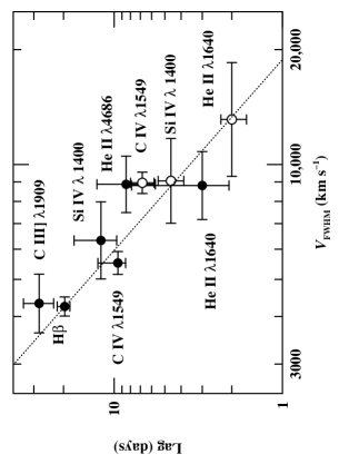
Figure 1: Inverse relationship between response time delay (lag) and the velocity measured of the variable broad emission line gas for NGC 5548 at two different epochs: 1989 and 1993. The dashed line shows the relationship for a virial mass of $6.8\times 10^{7}$ $M_{\odot}$. [Figure 1 of Peterson & Wandel (1999). Figure is courtesy of Brad Peterson.]

Second, it is not entirely clear that the issue with C iv is as bad as sometimes portrayed. The amplitude of the deviations reported between Mg ii and C iv mass estimates is for most studies of order 0.2$-$0.3 dex (e.g., Bachev et al. 2005; Baskin & Laor 2005. See also Vestergaard & Peterson 2006; Netzer et al. 2007), well within the uncertainties associated with the mass scaling laws. The most strongly deviating Mg ii and C iv mass estimates are seen for samples with a large fraction of low signal-to-noise data (e.g., Shen et al. 2008). The high signal-to-noise SDSS data that we use to calibrate the Mg ii scaling law do show a good correlation between the line widths of Mg ii and C iv; although some scatter is seen, the correlation between the mass measurements is somewhat stronger. It is worth keeping in mind that RM shows the C iv line gas to be virialized like the other emission lines. Note, however, that the C iv scaling law is not useful for narrow-line Seyfert 1 galaxies (Vestergaard 2004b).

Our work on all three emission lines shows that none of them are perfect; systematic differences are in fact seen in their profiles and their line widths. Indeed, we do see stronger deviations between line widths and mass estimates based on Mg ii and C iv than between H$\beta$ and Mg ii. But at present the issue has not been investigated well enough to firmly question the validity of C iv as a mass estimator. For example, could the dependence of the Mg ii profile width on the Eddington luminosity ratio (Onken & Kollmeier 2008) play a role here? We are in the process of investigating these issues regarding deviations between the mass scaling laws and will discuss our results in more detail in future work.

3 Black Hole Mass Functions

The differential quasar mass function is the space density of black holes per unit black hole mass as a function of redshift and black hole mass. We refer the interested reader to Vestergaard et al. (2008) and VO2009 for further details on the determination of the mass functions that we present here.

3.1 Why Are the Quasar Luminosity Functions Not Enough?

In the past, quasar luminosity distributions and luminosity functions have been used exclusively to constrain quasar and hence black hole evolution with cosmic time. So why do we even need the mass functions? It is worth keeping in mind that the luminosity is determined by the mass accretion rate. The accreted mass $dM/dt$ is converted into radiation with a certain efficiency $\eta$, defined by $L=\eta c^{2}dM/dt$. However, $L$ by itself does not tell us exactly how massive the central source is. For example, there is no way of knowing if a certain source is a low-mass black hole with a very large mass accretion rate, or whether it is a massive black hole with moderate accretion rate. By estimating the black hole masses we now know that most of the black holes in the distant universe are, in fact, quite massive (e.g., Vestergaard 2004a; Figure 1 of VO2009). If indeed the black holes we see as quasars were small but highly accreting we would expect to see narrow-lined quasars hovering right above the flux limits (dashed line in Figure 1 of VO2009) — the opposite of what we observe. To our knowledge there is nothing preventing us from detecting quasars with broad line widths of $\sim$1000 km s^-1 to 2500 km s^-1, yet we detect only very few of such sources among distant quasars. This is an important fact to keep in mind.

Another issue regarding the sole use of the luminosity function is the unknown value of the radiative efficiency $\eta$ and how it may change with time, type of source, and/or the evolutionary stage of the source — or, say, the spin of the black hole (e.g., Elvis et al. 2002). However, because $L$ is also a function of the black hole mass, the anticipation is that by combining our measurements of the luminosity and the mass of the black hole we can break the degeneracy that currently exists in our use of the luminosity function alone (Wyithe & Radmanabhan 2006) and perhaps even enable observational constraints to be placed on $\eta$.

3.2 Quasar Samples and Data

We present a summary of the mass functions of active black holes based on several large quasars samples recently published by Vestergaard et al. (2008) and VO2009: the SDSS DR3 quasar sample, the Bright Quasar Survey (BQS), the Large Bright Quasar Survey (LBQS), and the SDSS Fall Equatorial Stripe redshift 4 sample. The reader is referred to these works for details on the samples and the data. These samples are chosen because (a) a luminosity function has been established for each of them, (b) they each contain a large number of quasars, and (c) they complement each other well owing to the different selection criteria applied to the surveys in which they were found. Collectively, they cover a wide range of cosmic history, quasar properties, and a large part of the sky. For example, the SDSS survey is highly incomplete around redshifts of $z\sim 2$ to $z\sim 3$ due to the coincidence in color-space of quasars at those redshifts and the stellar locus. The LBQS of $\sim$1000 quasars complements well the SDSS since its quasars were selected based on SED shape in objective prism surveys. The implications are outlined later.

3.3 Sloan Digital Sky Survey DR3

Richards et al. (2006) present the luminosity function of a subset of about 15,000 DR3 quasars in a 1622 square degree area of the sky for which the selection function could be well established. They find a high-end slope of $\beta\approx-3.3$, and a steady decline in the amplitude from $z\sim 2$ to the local universe and from $z\sim 3$ to $z\sim 5$. For example, for a magnitude of $M_{i}=-27$ mag, the luminosity function has dropped by a factor of a few hundred between $z\sim 2$ and $z\sim 0.5$. This shows that the space density of quasars that are this luminous has dropped dramatically in the equivalent time span.

Figure 2: Mass function of actively accreting black holes in the SDSS DR3 quasar sample as a function of mass for different redshift bins. The dotted and dashed curves show, for reference, the observed mass functions at redshift bins of 0.49 and 2.01, respectively. The vertical (dashed and dotted) lines mark the black hole mass of a fiducial quasar with a luminosity at the SDSS flux limit and emission-line widths of 2000 km s^-1 and 3500 km s^-1, respectively.

Figure 2 shows the mass function for this sample. The characteristic turn-over toward low mass is mostly not real, but due to incompleteness. This is mainly caused by the fact that we do not select quasars for our surveys based on black hole mass, but on observed flux. For a given luminosity, a black hole can have a range of masses; in reality, a black hole of a given mass can have a range of luminosity because it may have a range of radiative efficiencies and/or mass accretion rates. The vertical lines denote the SDSS flux limits folded by, respectively, a line width of 2000 km s^-1 and 3500 km s^-1, the median H$\beta$ line width in the local universe. They indicate that most of the turn-over is due to incompleteness. Quasars are seen to lie below these crude limits because the observed total luminosities (used for source selection) also contain contributions from stars in the host galaxy plus iron and Balmer continuum emission in addition to the nuclear power-law continuum luminosity used for the mass estimates.

Figure 3: Random draws from the posterior probability density distribution of the underlying true black hole masses as established using Bayesian statistical methods that take into account the survey flux limits and uncertainties inherent in the mass estimates (light solid lines). The spread of the random draws illustrate the uncertainty in the mass functions. The lower limit in the selection function is located at the indent between the two Gaussian curves; the mass functions are most trustworthy rightward thereof. The binned mass functions from Figure 2 are shown as dots connected by solid lines. The dashed curve denotes the local mass function.

The high-mass end of the mass functions are nearly constant and those for black holes at $z\lesssim 3.5$ are all consistent with a slope of $\beta=-3.3$, similar to the luminosity functions. However, in contrast, the amplitude of the mass functions only changes by a factor of a few. The combination of the luminosity and mass functions thus show that the cumulative volume density of $L/M$ ($\propto L/L_{\rm Edd}$) decreases toward low redshift.

Because quasar surveys do not select sources based on black hole mass the binned mass functions shown in Figure 2 are statistically biased. We are currently using Bayesian statistical modeling to take the survey flux limits and the uncertainties in the mass scaling laws and on the spectral measurements into account (Kelly et al. 2008, 2009a, 2009b, and these proceedings). Our first (preliminary) results are in Figure 3 compared with the binned estimate of the mass functions. It is clear that the intrinsic mass function has a steeper high-end slope and higher peak amplitude than evidenced by the binned mass function. It is too preliminary to say whether the mass functions can be described by a single power-law, double power-law, or a Schecther function — that is, whether the bend right around the limit where the selection probability goes to zero value is real or not. The updated, final version of the mass function suggests that it is not real; see the published journal article of Kelly et al. 2009b).

3.4 Maximum Black Hole Mass

From our Bayesian analysis we constrain the maximum black hole mass of the mass distribution with high probability to lie between $\sim$1.5 and 4 billion $M_{\odot}$; such a black hole is most probably located at a redshift $z\sim 3$ (Kelly, these proceedings).

Figure 4: Mass functions of the active black holes (as a function of mass for different redshift bins) based on the quasar samples of the Large Bright Quasar Survey (LBQS), the Bright Quasar Survey (BQS), and the SDSS sample of redshift 4 quasars in the Fall Equatorial Stripe (marked as SDSS and referred to as the “SDSSz4” sample in the text). These mass functions are presented by Vestergaard & Osmer (2009) [VO2009].

3.5 The BQS, the LBQS, and the SDSS Fall Equatorial Stripe

In Figure 4, we compare the mass functions based on the BQS, the LBQS and the SDSS Fall Equatorial Stripe (hereafter, “the SDSSz4 sample”). The LBQS sample has been divided into smaller redshift bins. Similar to what we saw for the SDSS DR3 sample, the low-mass turn-over is due to incompleteness. In addition, the high-mass end slopes are very similar. For the samples below $z\sim 3$ (BQS and LBQS) the high-end slopes are consistent with $\beta\approx-3.3$ as seen for the DR3 mass function. Above $z=3.6$ (SDSSz4) the slope is shallower, $\beta\approx-1.8$ (see VO2009). There is also a marked difference in amplitude: the space density of $z\approx 4$ active black holes is lower than at $z\approx 2$. This is discussed below.

4 Evidence for Cosmic Downsizing

As noted earlier, the mass function is the space density of black holes as a function of both black hole mass and redshift. Because the SDSS DR3 sample is highly incomplete around $z\approx$ 2 (and the selection function is prone to be more uncertain there) this sample does not add valuable information to the mass function as a function of redshift. But, the LBQS allows us to probe this very well. In Figure 5 we show the space density distribution of black holes as a function of redshift for different mass bins, going from a mean black hole mass of $\sim 2.5\times 10^{8}$ $M_{\odot}$ (panel b) to a mean mass of $\sim 2.5\times 10^{10}$ $M_{\odot}$ (panel g). We see a steady progression of the maximum space density value from a low redshift to a higher redshift with increasing mass bin. This shows that the space density of active high-mass black holes was higher in the distant universe than it is in the local one and the most active black holes now are of low mass. This is what we typically refer to as “cosmic downsizing.” This “downsizing” trend appears to extend to the local universe: the mass function for local active black holes based on the Hamburg/ESO survey (Schulze & Wisotzki 2008; their Figure 4) shows a higher amplitude for $M_{\rm BH}<10^{8}$ $M_{\odot}$ than those based on LBQS and SDSS DR3 at $0.2\lesssim z\lesssim 0.5$ while the high-mass end slope ($\beta\approx-3.3$) is consistent with those of the LBQS and SDSS DR3 mass functions.

Figure 5: LBQS mass functions shown as a function of redshift for different mass bins. For a given mass bin, the redshift distribution shows at which epochs this active black hole is the most and least common. See Vestergaard & Osmer (2009) for the complete set of panels.

Figure 6: Mass functions (left panel) and cumulative mass density (right panel) for the BQS, LBQS, and SDSSz4 samples. In these diagrams the SDSSz4 mass function is extrapolated to very low masses and the implications for the cumulative mass density (open stars) is tested.

5 Evidence for Fast Build-up of the Black Hole Population at $z\sim 4$

We mentioned earlier that the mass function for the SDSSz4 sample has a distinctly different slope and amplitude compared to the LBQS and BQS mass functions at lower redshift (e.g., Figure 6, left panel). We also see a distinctly lower amplitude of the cumulative mass density (Figure 6, right panel) of this sample compared to the LBQS at $z\sim 2$ to $z\sim 3$. Could this be caused by our inability to detect the low-mass black holes (owing to the SDSS flux limits)? As a crude test thereof we extrapolated the SDSSz4 mass function to very low masses (dashed line in left panel) as a case study for the event that we were able to detect all black hole mass values. The result of integrating over the mass function and its extension is shown in the right panel as a dashed/asterics-dotted curve. This shows that our inability to detect black holes below a mass of $\sim 3\times 10^{8}$  $M_{\odot}$ does not explain the factor 10 lower cumulative mass density between $z\sim 4$ to $z\sim 2$ as seen in the right panel. In order for the cumulative mass density at $z\sim 4$ to approach that at lower redshift, the distribution of low-mass black holes has to be somewhat steeper than that indicated by the dashed line in the left panel. While future work will have to test such a scenario, we do not consider this very likely. Rather, the differences in mass functions and cumulative mass density between $z\sim 4$ and $z\sim 2$ suggest that a significant mass growth takes place during this time span.

The low-mass extension of the SDSSz4 mass function is parallel to the slope (dotted line, left panel) that the LBQS mass functions appear to move along with redshift. This amplitude difference between the dotted and dashed lines shows that on average the black hole space density needs to increase by about a factor of 17 from $z\sim 4$ to $z\sim 2$. We note, tongue in cheek, that while the quasar luminosity functions also show a strong decline in space density of luminous quasars with increasing redshift, this decline can just as well be explained by a decline in the number density of active black holes as a decline in their luminosities with redshift. The mass functions help confirm that a space density decline and a mass density decline (i.e., the typical mass of the black holes declines) is taking place.