On bulk viscosity and moduli decay

Abstract

This pedagogically intended lecture, one of four under the header “Basics of thermal QCD”, reviews an interesting relationship, originally pointed out by Bödeker, that exists between the bulk viscosity of Yang-Mills theory (of possible relevance to the hydrodynamics of heavy ion collision experiments) and the decay rate of scalar fields coupled very weakly to a heat bath (appearing in some particle physics inspired cosmological scenarios). This topic serves, furthermore, as a platform on which a number of generic thermal field theory concepts are illustrated. The other three lectures (on the QCD equation of state and the rates of elastic as well as inelastic processes experienced by heavy quarks) are recapitulated in brief encyclopedic form.

1 Introduction and outline

It has been a longstanding dream that experimental tests of thermal QCD through heavy ion collision experiments could yield theoretical insights that would be useful for some cosmological problems as well. These lectures covered selected topics within thermal QCD with this perspective in mind. The observables touched upon were the equation of state, shear and bulk viscosities, as well as the rates of elastic and inelastic reactions experienced by heavy quarks. Depending on the observable the focus was either on elaborating on the basic concepts, on outlining the link between heavy ion collisions and cosmology, or on reviewing modern developments.

Because of severe page limitations, it is not possible to cover all of the lectures in a detailed from in the proceedings. Rather, the choice has been made to concentrate on the second lecture, which is presented in some detail. The second lecture has been chosen because, first of all, the topic is rather elegant and concise, yet apparently little-known. Furthermore, it offers an opportunity to present a result which to my knowledge is original, generalizing the analysis of ref. [1] from a scalar field theory to a Yang-Mills theory. Finally, this topic can serve as a simple example permitting to introduce several tools (Kubo relations, Euclidean and Minkowskian correlators, the concept of transport coefficients) that are applicable much more widely in thermal field theory than to the very problem at hand.

The presentation is organized as follows. In section 2 we review the current theoretical understanding concerning the equation of state of QCD and the role that it may play in heavy ion collisions and in cosmology. Section 3, the main part of this presentation, concentrates on the topic announced in the title. The subject of section 4 is the rate of kinetic thermalization of heavy quarks, caused by elastic scatterings with the light degrees of freedom in the hot plasma. Finally, in section 5, recent developments in thermal heavy quarkonium physics, which to some extent can also be associated with the rate of inelastic processes felt by heavy quarks, are reviewed.

2 Lecture 1: QCD equation of state

In cosmology, it is in general an excellent approximation to set the baryon chemical potential to zero, so that thermodynamic potentials are functions of the temperature, $T$, only. Then the expansion rate of the system and the production rates of weakly interacting particles from the thermal medium (such as Dark Matter) depend on $p(T),p^{\prime}(T)$ and $p^{\prime\prime}(T)$, where $p(T)$ denotes the pressure [2]. The same functions (save without the contribution of photons and leptons, which have no time to thermalize) dictate the expansion of the thermal fireball created in an energetic heavy ion collision. Hence the longstanding efforts, both analytic (via chiral perturbation theory at low temperatures, $T\ll 200$ MeV, and the weak-coupling expansion at high temperatures, $T\gg 200$ MeV) and numerical (via lattice Monte Carlo simulations), to reliably determine these functions. At temperatures below one GeV, relevant for heavy ion collisions, the major qualitative finding, all but dashing early hopes of a spectacular scenario [3], has been that there is probably no phase transition at any $T$, only a smooth crossover.[4] Nevertheless large-scale numerical efforts to determine $p(T)$ and its derivatives for physical QCD in the infinite-volume and continuum limit go on. At temperatures above a few GeV, relevant for cosmology (only exceptional scenarios operate below this temperature range [5]), the system should be addressable with weak-coupling techniques. Perturbation theory does suffer from serious infrared problems, however: besides proceeding in powers of $\alpha_{s}^{\scriptscriptstyle 1/2}$ rather than $\alpha_{s}$,[6] it also comes with non-perturbative coefficients starting at the order $\alpha_{s}^{3}$.[7] That some coefficients are non-perturbative does not mean that they are beyond reach: indeed the non-perturbative input [8] can be determined via the use of effective field theory techniques [9]. As of today the non-perturbative part of the $\alpha_{s}^{3}$-term is known,[10] and it is possible to compile (systematically improvable) phenomenological values for $p(T),p^{\prime}(T)$ and $p^{\prime\prime}(T)$ of the Standard Model, applicable in the whole temperature range from $\sim$ GeV up to a few hundred GeV[11], or even higher if necessary.[12]

3 Lecture 2: bulk and shear viscosities

As a second example on the interplay between heavy ion collision experiments, cosmology, weak-coupling thermal field theory, and non-perturbative lattice simulations, we discuss observables known as the bulk and shear viscosities.

3.1 Phenomenological background

The bulk and shear viscosities are, in general, functions of the temperature and chemical potentials and parameterize gradient corrections to the energy-momentum tensor of a multiparticle system close to thermal equilibrium. At zeroth order in the gradient expansion one considers a system in which the temperature, $T$, and the four-velocity of the (“one-component”) medium, $u^{\mu}$, are constant in temporal and spatial coordinates; then the energy-momentum tensor, $T^{\mu\nu}$, is constructed out of symmetric and covariant structures proportional to the metric tensor, $g^{\mu\nu}$, and to $u^{\mu}u^{\nu}$. At first order in gradients, the structure $\partial^{\mu}u^{\nu}+\partial^{\nu}u^{\mu}$ can appear as well. Thus, $T^{\mu\nu}$ has the form (see, e.g., ref. [13])

$$T^{\mu\nu}=(p+e)u^{\mu}u^{\nu}-p\,g^{\mu\nu}+{\mathcal{O}}((\eta,\zeta)(\partial^{\mu}u^{\nu}+\partial^{\nu}u^{\mu}))\;.$$ (1)

Here $p$ denotes the pressure, $e$ the energy density, $\eta$ the “shear” viscosity, and $\zeta$ the “bulk” viscosity, and the metric convention ($+$$-$$-$$-$) was assumed. The equation of motion reads $\partial_{\mu}T^{\mu\nu}=0$.

More precisely, the shear viscosity coefficient $\eta$ is defined to be a function that multiplies the traceless part of the leading gradient correction; the bulk viscosity coefficient $\zeta$ multiplies the trace part. The explicit forms of the corresponding structures are most simply displayed in a non-relativistic frame, $|u^{i}|\ll 1$; then

$$T_{ij}\approx(p-\zeta\nabla\cdot{\bf v})\delta_{ij}-\eta(\partial_{i}v^{j}+\partial_{j}v^{i}-{\frac{2}{3}}\delta_{ij}\nabla\cdot{\bf v})\;,$$ (2)

where $\nabla\cdot{\bf v}=\partial_{i}v^{i}$ and $\delta_{ij}$ is the usual Kronecker symbol.

Now, since the system generated in a heavy ion collision is relatively small, gradients can be large, with a scale given by the system size:

$$\left(\frac{\partial u}{u}\right)^{-1}\sim{\mbox{few~{}fm}}\sim\frac{\mbox{few}}{T_{\mbox{\tiny\rm{QCD}}}}\;,$$ (3)

where $T_{\mbox{\tiny\rm{QCD}}}\equiv 200$ MeV. In the relativistic limit, $\eta\sim T^{3}$ and $p\sim T^{4}$; this then implies that $\eta\,\partial u\sim p\,u^{2}$. In other words, gradient corrections could be as large as the leading terms. Setting aside the question of whether a gradient expansion can be justified at all in this situation, it seems conceivable that the viscosities could indeed affect the expansion of the thermal fireball created in a heavy ion collision. An example on the effects of the shear viscosity on the azimuthal anisotropies of particle spectra produced in a heavy ion collision can be found in ref. [14] while possible implications of a (large) bulk viscosity have been explored in, e.g., ref. [15].

We now turn to cosmology. An immediate qualitative difference between the matter created in a heavy ion collision and that filling the Early Universe is that the latter system is rather homogeneous. For instance, if we are interested in the overall expansion, then the system size can be identified with the horizon radius, which in the QCD epoch ($T\sim T_{\mbox{\tiny\rm{QCD}}}$) is

$$\ell_{H}\sim t\sim\frac{m_{\mbox{\scriptsize Planck}}}{T^{2}}\sim\frac{10^{20}}{T_{\mbox{\tiny\rm{QCD}}}}\;.$$ (4)

This can be contrasted with eq. (3); thus gradient corrections are bound to be insignificant as far as the overall expansion is concerned. (Nevertheless, there may be other physics questions for which they do play a role; indeed some inhomogeneities do exist within the horizon, as is famously indicated by anisotropies in the cosmic microwave background and as is required for successful large-scale structure formation. In spite of the fact that at early times their relative magnitude is of order $\sim 10^{-5}$ rather than of order unity, viscosities might still affect the evolution of density perturbations; see, e.g., refs. [16, 17].)

It turns out, however, that the bulk viscosity $\zeta$ makes a formal appearance in a completely different context.[1] In order to discuss this, we need to next recall some basic facts concerning the important role that scalar fields play in cosmology.

3.2 Scalar fields and the moduli problem in cosmology

Although no fundamental scalar fields have been experimentally discovered up to date, they play a very important role in inflationary cosmology, and are also considered to be a generic feature of many models inspired by string theory or supersymmetry. At an early stage, it is assumed that a significant amount of energy may be stored in the scalar fields. Later on, as the Universe enters the radiation dominated epoch, the scalar fields should “decay”, i.e. transform their energy to the known particles (electrons, photons, etc); this is called a reheating period. It is possible to imagine scalar fields, however, which are coupled so weakly that they decay later than the inflaton field, or not at all. In the case of a delayed decay, one may use the scalar field to generate a possibly observable “second” component of density perturbations; such a scalar field is often called a “curvaton”. Yet if the decay is too slow and the scalar field does not get rid of its energy density at all, it eventually becomes a dominant component, in conflict with observation. Such a situation is met particularly in connection with scalar fields called moduli, and the problem of their slow decay is the “moduli problem”.

We note, in passing, that there are many other similar “dangerous relics” in cosmology: in particular theories predicting the generation of topological defects in the form of domain walls or monopoles are practically excluded, if the associated energy scale corresponds to physics beyond the Standard Model.

To be concrete, let us consider a toy model in which a scalar field, $\varphi$, couples to Yang-Mills fields:

$$\mathcal{L}={\frac{1}{2}}\varphi(-\square-m^{2})\varphi-\frac{1}{4g^{2}}F^{a\mu\nu}F^{a}_{\mu\nu}-\frac{\varphi}{M}\times F^{a\mu\nu}F^{a}_{\mu\nu}\;,$$ (5)

where $m$ is some “small” mass scale, perhaps $m\sim m_{\mbox{\scriptsize SUSY}}$, while $M$ is some large scale, perhaps $M\sim m_{\mbox{\scriptsize Planck}}$. The non-renormalizable coupling between $\varphi$ and the Yang-Mills fields is suppressed by the heavy mass scale; hence the coupling between the two sets of fields is very weak. In ref. [1] a similar system was considered, however the scalar field $\varphi$ was coupled to another scalar field, denoted by $\chi$.

If we now assume that the initial state of the system is such that $\langle\varphi(0)\rangle\gg m$, then the initial energy density in the scalar field is $e_{\varphi}\gg m^{4}$. According to eq. (5) the scalar field can decay to gauge bosons; however the coupling is suppressed by $M$, so the (vacuum) decay rate is $\Gamma\sim m^{3}/M^{2}$. The corresponding time scale, $t_{\varphi}\sim M^{2}/m^{3}$, can be contrasted with that in eq. (4); it is known from observation that a conventional radiation-dominated expansion is needed at least starting from the nucleosynthesis epoch ($T\sim T_{\mbox{\scriptsize n}}\equiv 0.1$ MeV). (For completeness, a cartoon of a standard cosmological scenario is attached as fig. 1.) If $M\sim m_{\mbox{\scriptsize Planck}}$, the corresponding constraint $t_{\varphi}\ll t_{\mbox{\scriptsize n}}$ translates to $m\gg(m_{\mbox{\scriptsize Planck}}T_{\mbox{\scriptsize n}}^{2})^{1/3}\sim 10$ TeV. While not impossible, this looks unattractive if $m$ is to be related, for instance, to some lifted SUSY flat direction.

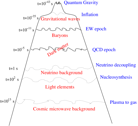
Figure 1: A cartoon of a possible cosmological scenario. The age of the Universe, $t$, and the temperature of the plasma filling it, $T$, are related through $t[\mbox{s}]\sim(T[\mbox{MeV}])^{-2}$ (cf. eq. (4)).

3.3 Decay rate in thermal field theory

The question now is, could the vacuum decay rate ($\Gamma\sim m^{3}/M^{2}$) be modified by thermal corrections associated with the “normal” degrees of freedom, represented by $F^{a}_{\mu\nu}$? In particular, could the thermal plasma be “viscous” enough to dissipate the energy related to the oscillations of the “dangerous relic” $\varphi$ well before the nucleosynthesis epoch, rendering $\varphi$ harmless even if the mass $m$ were only in the TeV range or below it?

In order to answer this question, let us consider the equation of motion satisfied by $\varphi$. In the temperature range $m\ll T\ll M$, the scalar field is “light” and oscillates slowly compared with the typical frequencies of the thermal degrees of freedom. In this situation, we can assume that the “fast” thermal fields see $\varphi$ essentially as a constant, and have time to adjust to any given value. From their perspective, then, the system remains in thermal equilibrium, only in the presence of a background field $\varphi$. From the perspective of $\varphi$, on the other hand, the net effect of the thermal medium is to exert some friction which slows down its oscillations. Focussing on the infrared modes of $\varphi$ (the modes with the slowest temporal and spatial variations), we can expect an equation of motion of the form

$$\square\varphi+V_{\mbox{\scriptsize eff}}^{\prime}(\varphi)=-\Gamma\dot{\varphi}+{\mathcal{O}}(\raise-1.49994pt\hbox{$\stackrel{{\scriptstyle\dots}}{{\varphi}}$},\nabla^{2}\dot{\varphi},\dot{\varphi}^{2},(\nabla\varphi)^{2})\;.$$ (6)

The main task then is to determine the coefficient $\Gamma$ (although we will also discuss thermal corrections to $V_{\mbox{\scriptsize eff}}$, particularly through a mass parameter $m_{\mbox{\scriptsize eff}}^{2}$).

Now, a standard tool in thermal field theory is a “Kubo formula”, which indeed allows to determine “response” or “transport” coefficients of the same type as $\Gamma$. Note that $\Gamma$ as defined by eq. (6) is, by construction, a constant. It is given by

$$\Gamma=\lim_{\omega\to 0}\frac{\rho(\omega,{\bf 0})}{\omega}\;,$$ (7)

where, for $\mathcal{L}_{\mbox{\scriptsize int}}=-\varphi H_{\mbox{\scriptsize int}}$, $\rho$ is a spectral function related to the operator $\hat{H}_{\mbox{\scriptsize int}}$:

$$\rho(\omega,{\bf 0})\equiv\int_{t,{\bf x}}e^{i\omega t}\left\langle{\frac{1}{2}}\left[\hat{H}_{\mbox{\scriptsize int}}(t,{\bf x}),\hat{H}_{\mbox{\scriptsize int}}(0,{\bf 0})\right]\right\rangle\;.$$ (8)

The expectation value is taken with respect to the density matrix of the “normal” degrees of freedom which, as alluded to above, can be assumed to be thermalized.

• Sketch of a proof of eq. (7)

  Let us consider the form of eq. (6) in Fourier space, with $\varphi\propto e^{-i\omega t+i{\bf p}\cdot{\bf x}}\;\tilde{\varphi}$:

  $$[-\omega^{2}+{\bf p}^{2}+m_{\mbox{\scriptsize eff}}^{2}-i\omega\Gamma+{\mathcal{O}}(\omega^{3},\omega{\bf p}^{2})]\tilde{\varphi}={\mathcal{O}}(\tilde{\varphi}^{2})\;.$$ (9)

  We compare the dispersion relation from here with the “pole” appearing in the Euclidean propagator of $\tilde{\varphi}$ after the analytic continuation $\omega_{n}\to-i(\omega+i0^{+})$:

  $$\frac{1}{\omega_{n}^{2}+{\bf p}^{2}+\Pi_{E}}\to\frac{1}{-\omega^{2}-i\omega 0^{+}+{\bf p}^{2}+\mathop{\rm Re}\Pi_{E}+i\mathop{\rm Im}\Pi_{E}}\;.$$ (10)

  Taking ${\bf p}\to{\bf 0}$ and denoting $m_{\mbox{\scriptsize eff}}^{2}\equiv\mathop{\rm Re}\Pi_{E}(-i[\omega+i0^{+}],{\bf 0})$, we can identify

  $$\Gamma=-\lim_{\omega\to 0}\frac{\mathop{\rm Im}\Pi_{E}(-i[\omega+i0^{+}],{\bf 0})}{\omega}\;.$$ (11)

  It remains to note that, as can be verified with basic path integral techniques in Euclidean spacetime,

  $$\Pi_{E}(\omega_{n},{\bf p})=-\int_{\tau,{\bf x}}e^{i\omega_{n}\tau+i{\bf p}\cdot{\bf x}}\left\langle H_{\mbox{\scriptsize int}}(\tau,{\bf x})\,H_{\mbox{\scriptsize int}}(0,{\bf 0})\right\rangle\;,$$ (12)

  where $0\leq\tau\leq 1/T$, and that its imaginary part yields

  $$\mathop{\rm Im}\Pi_{E}(-i[\omega+i0^{+}],{\bf 0})=-\rho(\omega,{\bf 0})\;,$$ (13)

  with $\rho$ defined through the commutator in eq. (8); eq. (13) will be justified presently. This completes the proof of eq. (7).

Before proceeding to prove eq. (13), let us pause to contemplate an important point. The oscillation frequency given by eq. (9) does not vanish, but is rather given by (for ${\bf p}\to{\bf 0}$)

$$\omega^{2}\approx m_{\mbox{\scriptsize eff}}^{2}\sim m^{2}+\frac{T^{4}}{M^{2}}\;,$$ (14)

where we have also included a thermal correction from the interaction in eq. (5). Why is it then that $\Gamma$ of eq. (7) is evaluated at vanishing frequency? The reason is that $\rho(\omega,{\bf 0})/\omega$ shows generically a transport peak at origin, resembling a smoothed Dirac $\delta$-function: it has the height $\Gamma$ and a width, $\eta$, determined by the scales of the thermal system. For Yang-Mills theory, parametrically, $\eta\sim g^{4}T$ [18]. In the range $m\ll T\ll M$ that we are interested in, however, $m_{\mbox{\scriptsize eff}}\ll T$ according to eq. (14). Therefore, if $g$ is not exceedingly small, $m_{\mbox{\scriptsize eff}}\ll\eta\sim g^{4}T$, and we can well approximate $\rho(m_{\mbox{\scriptsize eff}},{\bf 0})/m_{\mbox{\scriptsize eff}}$ by its limit $\lim_{\omega\to 0}\rho(\omega,{\bf 0})/\omega$, simplifying the problem and obtaining in any case the largest (i.e. most optimistic) $\Gamma$.

• Sketch of a proof of eq. (13)

  Apart from the usual Heisenberg operators $\hat{A}(t)=e^{i\hat{H}t}\hat{A}(0)e^{-i\hat{H}t}$ it is convenient to define “imaginary-time” Heisenberg operators as $\hat{A}(\tau)\equiv e^{\hat{H}\tau}\hat{A}(0)e^{-\hat{H}\tau}$, where $0\leq\tau\leq\beta$, $\beta\equiv 1/T$. We furthermore define the correlators

  $$\Pi_{>}(\omega) \equiv \int_{-\infty}^{\infty}\!{\rm d}t\,e^{i\omega t}\Bigl{\langle}\hat{A}(t)\hat{A}(0)\Bigl{\rangle}\;,$$ (15)

  $$\Pi_{<}(\omega) \equiv \int_{-\infty}^{\infty}\!{\rm d}t\,e^{i\omega t}\Bigl{\langle}\hat{A}(0)\hat{A}(t)\Bigl{\rangle}\;,$$ (16)

  $$\rho(\omega) \equiv \int_{-\infty}^{\infty}\!{\rm d}t\,e^{i\omega t}\left\langle{\frac{1}{2}}\Bigl{[}\hat{A}(t),\hat{A}(0)\Bigr{]}\right\rangle\;,$$ (17)

  $$G_{E}(\tau) \equiv \Bigl{\langle}\hat{A}(\tau)\hat{A}(0)\Bigl{\rangle}\;,$$ (18)

  $$\tilde{G}_{E}(\omega_{n}) \equiv \int_{0}^{\beta}\!{\rm d}\tau\,e^{i\omega_{n}\tau}G_{E}(\tau)\;;\quad\omega_{n}\equiv 2\pi nT\;,\quad n\in{\mathbb{Z}}\;.$$ (19)

  Here the expectation value is $\langle...\rangle\equiv\frac{1}{\mathcal{Z}}\mathop{\rm Tr}\{e^{-\beta\hat{H}}(...)\}$, and it is easy to see that $G_{E}(\beta-\tau)=G_{E}(\tau)$, i.e. $G_{E}(\tau)$ is periodic. Spatial directions have been suppressed for simplicity but are trivial to incorporate. The correlator $G_{E}(\tau)$ is theoretically a nice object, because it can be given a Euclidean path integral representation and thus a direct non-perturbative meaning.

  Inserting twice $\mathbbm{1}=\sum_{n}|n\rangle\langle n|$ in eqs. (15), (16), it is straightforward to show that $\Pi_{<}(\omega)=e^{-\beta\omega}\Pi_{>}(\omega)$. It then follows that

  $$\rho(\omega)={\frac{1}{2}}\left[\Pi_{>}(\omega)-\Pi_{<}(\omega)\right]={\frac{1}{2}}\left(1-e^{-\beta\omega}\right)\Pi_{>}(\omega)\;,$$ (20)

  or, conversely, that $\Pi_{>}(\omega)=2\rho(\omega)/(1-e^{-\beta\omega})$. Making use of the fact that, through their definitions as correlators of Heisenberg operators, $G_{>}(t)$ and $G_{E}(\tau)$ are related by the analytic continution $\tau\leftrightarrow it$, we finally obtain

  $$\tilde{G}_{E}(\omega_{n}) = \int_{0}^{\beta}\!{\rm d}\tau\,e^{i\omega_{n}\tau}\biggl{[}\int_{-\infty}^{\infty}\!\frac{{\rm d}\omega}{2\pi}\,e^{-i\omega t}\Pi_{>}(\omega)\biggr{]}_{it\to\tau}$$ (21)

  $$= \int_{0}^{\beta}\!{\rm d}\tau\,e^{i\omega_{n}\tau}\int_{-\infty}^{\infty}\frac{{\rm d}\omega}{2\pi}e^{-\omega\tau}\Pi_{>}(\omega)$$

  $$= \int_{0}^{\beta}\!{\rm d}\tau\,e^{i\omega_{n}\tau}\int_{-\infty}^{\infty}\frac{{\rm d}\omega}{2\pi}e^{-\omega\tau}\frac{2\rho(\omega)}{1-e^{-\beta\omega}}$$

  $$= \int_{-\infty}^{\infty}\frac{{\rm d}\omega}{\pi}\frac{\rho(\omega)}{1-e^{-\beta\omega}}\left[\frac{e^{(i\omega_{n}-\omega)\tau}}{i\omega_{n}-\omega}\right]^{\beta}_{0}$$

  $$= \int_{-\infty}^{\infty}\frac{{\rm d}\omega}{\pi}\frac{\rho(\omega)}{1-e^{-\beta\omega}}\frac{e^{-\beta\omega}-1}{i\omega_{n}-\omega}$$

  $$= \int_{-\infty}^{\infty}\!\frac{{\rm d}\omega}{\pi}\frac{\rho(\omega)}{\omega-i\omega_{n}}\;.$$

  (To be precise, the validity of eq. (21) requires the presence of an ultraviolet regulator for spatial momenta, guaranteeing that both $\rho(\omega)$ and $\tilde{G}_{E}(\omega_{n})$ are cut off at large values of the argument.) Equation (13) now follows by noting that the relation

  $$\frac{1}{x\pm i0^{+}}=P\left(\frac{1}{x}\right)\mp i\pi\delta(x)$$ (22)

  implies that

  $$\mathop{\rm Im}\tilde{G}_{E}\left(-i[\omega+i0^{+}]\right)=\rho(\omega)\;,$$ (23)

  and by then inserting $-\Pi_{E}(\omega_{n},{\bf p})$ from eq. (12) for $\tilde{G}_{E}(\omega_{n})$.

3.4 Relation of the decay rate $\Gamma$ to the bulk viscosity $\zeta$

Let us now consider the specific case of eq. (5), viz.

$$H_{\mbox{\scriptsize int}}=\frac{1}{M}F^{a\mu\nu}F^{a}_{\mu\nu}\;.$$ (24)

At this point it is good to realize that the structure appearing can be recognized as the “trace anomaly” of pure Yang-Mills theory,

$$\Theta={T^{\mu}}_{\mu}\approx-\frac{b_{0}}{2}\,F^{a\mu\nu}F^{a}_{\mu\nu}\;,$$ (25)

where $b_{0}$ defines the $\beta$-function related to the running coupling, $b_{0}=11N_{\rm c}/3(4\pi)^{2}$.

• Sketch of a proof of eq. (25)

  With the convention

  $$S=\int\!{\rm d}t\int\!{\rm d}^{3-2\epsilon}{\bf x}\,\left\{-\frac{1}{4g_{\mbox{\tiny\rm{B}}}^{2}}F^{a\mu\nu}F^{a}_{\mu\nu}\right\}$$ (26)

  the energy-momentum tensor is

  $$T_{\mu\nu}=\frac{1}{g_{\mbox{\tiny\rm{B}}}^{2}}\left({\frac{1}{4}}g_{\mu\nu}F^{a\alpha\beta}F^{a}_{\alpha\beta}-{F^{a\alpha}}_{\mu}F^{a}_{\alpha\nu}\right)\;.$$ (27)

  In ${\delta^{\mu}}_{\mu}=4-2\epsilon$ dimensions its trace is

  $${T^{\mu}}_{\mu}=-\frac{2\epsilon}{4}\frac{1}{g_{\mbox{\tiny\rm{B}}}^{2}}F^{a\alpha\beta}F^{a}_{\alpha\beta}\;.$$ (28)

  The inverse of the bare gauge coupling ($g_{\mbox{\tiny\rm{B}}}^{2}=g^{2}-\frac{11N_{\rm c}}{3\epsilon}\frac{g^{4}}{(4\pi)^{2}}+{\mathcal{O}}(g^{6})$) is
  

  $$\frac{1}{g_{\mbox{\tiny\rm{B}}}^{2}} = \frac{1}{g^{2}}+\frac{11N_{\rm c}}{3\epsilon}\frac{1}{(4\pi)^{2}}+{\mathcal{O}}\left(\frac{g^{2}}{\epsilon}\right)\;.$$ (29)

  So, in the limit $\epsilon\to 0$,

  $${T^{\mu}}_{\mu}\approx-\frac{11N_{\rm c}}{6}\frac{1}{(4\pi)^{2}}F^{a\alpha\beta}F^{a}_{\alpha\beta}\;.$$ (30)

Returning to eqs. (24), (25), we see that $H_{\mbox{\scriptsize int}}=F^{a\mu\nu}F^{a}_{\mu\nu}/M\approx-2\Theta/b_{0}M$. Therefore eqs. (7), (8) advise us to determine the transport coefficient related to the trace anomaly. However, as mentioned after eq. (1), the trace of the energy-momentum tensor is intimately related to bulk viscosity: in fact the latter can be expressed through another Kubo relation,

$$\zeta=\frac{1}{9}\lim_{\omega\to 0}\frac{1}{\omega}\int_{t,{\bf x}}e^{i\omega t}\left\langle{\frac{1}{2}}\left[\hat{\Theta}(t,{\bf x}),\hat{\Theta}(0,{\bf 0})\right]\right\rangle\;.$$ (31)

Furthermore, motivated by the hydrodynamics of heavy ion collision experiments, the weak-coupling expression for $\zeta$ has been worked out,[19]

$$\zeta\sim\frac{b_{0}^{2}g^{4}T^{3}}{4\ln(1/\alpha_{s})}\;,\quad\alpha_{s}\equiv\frac{g^{2}}{4\pi}\;.$$ (32)

As the appearance of $\ln(1/\alpha_{s})$ in the denominator suggests, the computation is very non-trivial and necessitates a systematic resummation of the perturbative series. (Taking the Euclidean formulation as a starting point, there are also attempts at a non-perturbative determination of $\zeta$ in the temperature regime where the weak-coupling expansion can no longer be justified.[20])

In conclusion, combining eqs. (7), (8), (31), (32) and the relation $H_{\mbox{\scriptsize int}}\approx-2\Theta/b_{0}M$, the vacuum decay rate of the moduli fields, $\Gamma\sim{m^{3}}/{M^{2}}$, is overtaken at $m\ll T\ll M$ by a thermal correction:

$$\Gamma = \lim_{\omega\to 0}\frac{1}{\omega}\int_{t,{\bf x}}e^{i\omega t}\left\langle{\frac{1}{2}}\left[\hat{H}_{\mbox{\scriptsize int}}(t,{\bf x}),\hat{H}_{\mbox{\scriptsize int}}(0,{\bf 0})\right]\right\rangle$$ (33)

$$\approx \frac{4\times 9\,\zeta}{b_{0}^{2}M^{2}}\;\sim\;\frac{(12\pi\alpha_{s})^{2}}{\ln(1/\alpha_{s})}\frac{T^{3}}{M^{2}}\;\;{\gg}\;\;\frac{m^{3}}{M^{2}}\;.$$

In other words, the fact that there is already a plasma present “facilitates” the dissipation of the energy in the scalar field $\varphi$ into that in normal radiation.

3.5 Implications for the moduli problem

We finally contemplate whether the rate in eq. (33) could be fast enough to solve the cosmological moduli problem. Since the rate increases with $T$, we first need to figure out the initial temperature at which the oscillations start. To do this properly we would need to rewrite eq. (6) in an expanding background, but the upshot is that oscillations start once their frequency exceeds the Hubble rate (the inverse of eq. (4)):

$$m_{\mbox{\scriptsize eff}}\mathop{\raise 1.29167pt\hbox{$>$\kern-7.5pt\raise-4.73611pt\hbox{$\sim$}}}\frac{T^{2}}{m_{\mbox{\scriptsize Planck}}}\;\Rightarrow\;T\mathop{\raise 1.29167pt\hbox{$<$\kern-7.5pt\raise-4.73611pt\hbox{$\sim$}}}\sqrt{\rule{0.0pt}{8.61108pt}m_{\mbox{\scriptsize eff}}\,m_{\mbox{\scriptsize Planck}}}\sim\sqrt{mM}\;.$$ (34)

Then we should integrate the energy loss equation all the way down to the temperature $T\sim m$ at which point the vacuum decay takes over. We note, however, that within all of this range the decay rate falls far below the Hubble rate:

$$\frac{(12\pi\alpha_{s})^{2}}{\ln(1/\alpha_{s})}\frac{T^{3}}{M^{2}}\ll\frac{T^{2}}{M}$$ (35)

because, according to eq. (34), $T/M\mathop{\raise 1.29167pt\hbox{$<$\kern-7.5pt\raise-4.73611pt\hbox{$\sim$}}}\sqrt{m/M}\ll 1$. Therefore, the decay is so slow that it essentially does not have time to take place within the lifetime of the Universe; thermal corrections quite probably cannot solve the moduli problem.[1]

3.6 Summary

The purpose of this lecture has been to illustrate various generic tools of thermal field theory, as well as the intriguing fact that systematic heavy ion collision inspired computations may find “exciting” applications in totally unexpected cosmological contexts. In the present example we could learn this way that the moduli problem remains a severe constraint even in the presence of thermal corrections, a fact to be taken into account in cosmological model building.

4 Lecture 3: heavy quark kinetic thermalization

The production of a heavy quark and antiquark through gluon fusion, which then fly apart in opposite directions, is one of the most basic processes in a hadronic collision. In the heavy ion case, the “flying apart” part is non-trivial, however, due to the presence of a thermal medium which the heavy quarks have to surpass. The process is akin to Brownian motion, whereby the heavy quarks gradually lose their kinetic energy through collisions with the medium particles.[21, 22] This physics can be referred to as heavy quark kinetic thermalization, diffusion, momentum diffusion, drag, jet quenching, stopping, or energy loss. The situation becomes particularly tractable if we focus on a “late stage” of the process, in which the heavy quarks are non-relativistic with respect to the heat bath; then it can be described by Langevin dynamics, with the role of the stochastic noise being played by the colour-electric Lorentz force. Through a QCD generalization of the fluctuation-dissipation theorem the problem thus boils down to the consideration of the 2-point temporal correlation function of the colour-electric field strength (rendered gauge-invariant by time-like Wilson lines).[23, 24] The “transport coefficient” extracted from this correlator, conventionally referred to as $\kappa$, has been the subject of some recent interest. A leading-order weak-coupling result[25] has been supplemented by a next-to-leading order correction [26], which has however been shown to be so large as to question the validity of the weak-coupling expansion. Numerical simulations have been carried out within so-called classical lattice gauge theory, confirming the existence of large infrared effects.[27] Computations through AdS/CFT techniques for similar processes in strongly coupled $\mathcal{N}=4$ Super-Yang-Mills theory also suggest a much larger $\kappa$ than expected in leading-order QCD [23, 28]. All of this makes a strong case for attacking the problem with lattice simulations, a challenge that appears technically simpler than in the case of many other transport coefficients such as viscosities.[29] If an answer can be obtained, it can be embedded in hydrodynamic simulations of heavy ion collisions (e.g. ref. [30]) and eventually compared with experimental observations concerning the spectrum and azimuthal anisotropy of the decay products from heavy quarks.[31] In cosmology, an analogous kinetic thermalization also plays a role, given that many Dark Matter candidates kinetically decouple in a non-relativistic regime, and their momentum distribution dictates the kind of structures that can form.[17]

5 Lecture 4: quarkonium in hot QCD

Quarkonium physics in heavy ion collisions is somewhat similar to heavy quark physics discussed in the previous section, however in many ways more complicated: initial production is less likely because two heavy quarks and two heavy antiquarks need to be generated, and furthermore a quark and antiquark have to be in a suitable kinematic range in order to bind together; in addition propagation through the medium is affected by several processes, such as scatterings experienced by the quark–antiquark colour dipole, decoherence of the quantum-mechanical bound state caused by interactions with the medium, as well as Debye screening of the potential that binds the system together. Recently, some progress has been made in systematizing the study of these phenomena, by formulating the problem (implicitly or explicitly) in an effective field theory language. [32] The setup makes use of scale separations, such as $\alpha_{s}^{2}M\ll\alpha_{s}M\ll M$ at zero temperature, $\alpha_{s}T\ll\alpha_{s}^{\scriptscriptstyle 1/2}T\ll T$ at finite temperature, and an additional $\alpha_{s}M\ll T\ll\alpha_{s}^{\scriptscriptstyle 1/2}M$ to relate the two.[33] (It remains a challenge to promote the setup to the non-perturbative level.) An example of a generic feature emerging from the effective theory approach is that a concept of a static potential can be defined (as a “matching coefficient”), however it is static in Minkowskian rather than in Euclidean time. It is also complex unlike at zero temperature, with an imaginary part responsible for decoherence or, in frequency space, for the width of the quarkonium peak in the corresponding spectral function. Thus the static potential is different from that traditionally extracted from finite-$T$ lattice QCD, which is purely real and relies on gauge fixing to the Coloumb gauge. Recently, an interesting attempt has been launched to extract the proper real-time potential from the lattice,[34] however further work is needed before conclusions can be drawn. Another insight is that purely perturbative studies may converge much better than in general (cf. the previous section),[35] because only short-distance physics plays a role for heavy quarkonium. Ultimately, one of the goals of these efforts is to determine the spectrum of the dilepton pairs produced from thermal quarkonium decays[36] (given that quarks disappear we may refer to this as an inelastic process). A cosmological analogue may exist in near-threshold two-particle Dark Matter production or decay, relevant for some of the most popular scenarios.[2, 37]

References

- [1] D. Bödeker, \JLJCAP,06,2006,027, hep-ph/0605030.
- [2] P. Gondolo and G. Gelmini, \NPB360,1991,145.
- [3] E. Witten, \PRD30,1984,272.
-
[4]
P. de Forcrand and O. Philipsen,
\JHEP01,2007,077,
hep-lat/0607017.
Y. Aoki et al, \JLNature,443,2006,675, hep-lat/0611014. - [5] A. Boyarsky et al, \JLAnn. Rev. Nucl. Part. Sci.,59,2009,191, 0901.0011.
- [6] J.I. Kapusta, \NPB148,1979,461.
-
[7]
A.D. Linde,
\PLB96,1980,289.
D.J. Gross, R.D. Pisarski and L.G. Yaffe, \JLRev. Mod. Phys.,53,1981,43. - [8] A. Hietanen et al, \JHEP01,2005,013, hep-lat/0412008.
-
[9]
P. Ginsparg,
\NPB170,1980,388.
T. Appelquist and R.D. Pisarski, \PRD23,1981,2305. - [10] F. Di Renzo et al, \JHEP07,2006,026, hep-ph/0605042.
- [11] M. Laine and Y. Schröder, \PRD73,2006,085009, hep-ph/0603048.
- [12] A. Gynther and M. Vepsäläinen, \JHEP01,2006,060, hep-ph/0510375.
- [13] L.D. Landau and E.M. Lifshitz, Fluid mechanics, 2nd Edition (Pergamon, Oxford, 1987).
- [14] P. Romatschke and U. Romatschke, \PRL99,2007,172301, 0706.1522.
-
[15]
G. Torrieri, B. Tomasik and I. Mishustin,
\PRC77,2008,034903,
0707.4405.
K. Rajagopal and N. Tripuraneni, \JHEP03,2010,018, 0908.1785.
H. Song and U.W. Heinz, \PRC81,2010,024905, 0909.1549. - [16] Steven Weinberg, Gravitation and Cosmology (Wiley, New York, 1972).
- [17] S. Hofmann et al, \PRD64,2001,083507, astro-ph/0104173.
- [18] G.D. Moore and O. Saremi, \JHEP09,2008,015, 0805.4201.
- [19] P.B. Arnold, C. Dogan and G.D. Moore, \PRD74,2006,085021, hep-ph/0608012.
- [20] H.B. Meyer, \JHEP04,2010,099, 1002.3343.
- [21] B. Svetitsky, \PRD37,1988,2484.
- [22] E. Braaten and M.H. Thoma, \PRD44,1991,2625.
- [23] J. Casalderrey-Solana and D. Teaney, \PRD74,2006,085012, hep-ph/0605199.
- [24] S. Caron-Huot, M. Laine and G.D. Moore, \JHEP04,2009,053, 0901.1195.
- [25] G.D. Moore and D. Teaney, \PRC71,2005,064904, hep-ph/0412346.
- [26] S. Caron-Huot and G.D. Moore, \JHEP02,2008,081, 0801.2173.
- [27] M. Laine et al, \JHEP05,2009,014, 0902.2856.
-
[28]
C.P. Herzog et al, \JHEP07,2006,013,
hep-th/0605158.
S.S. Gubser, \PRD74,2006,126005, hep-th/0605182. - [29] Y. Burnier, M. Laine, J. Langelage and L. Mether, 1006.0867.
- [30] Y. Akamatsu, T. Hatsuda and T. Hirano, \PRC79,2009,054907, 0809.1499.
-
[31]
B.I. Abelev et al. [STAR],
\PRL98,2007,192301,
nucl-ex/0607012.
A. Adare et al. [PHENIX], \PRL98,2007,172301, nucl-ex/0611018. -
[32]
M. Laine et al, \JHEP03,2007,054,
hep-ph/0611300.
A. Beraudo, J.P. Blaizot and C. Ratti, \NPA806,2008,312, 0712.4394.
M.A. Escobedo and J. Soto, \PRA78,2008,032520, 0804.0691.
N. Brambilla et al, \PRD78,2008,014017, 0804.0993.
F. Dominguez and B. Wu, \NPA818,2009,246, 0811.1058. - [33] Y. Burnier, M. Laine and M. Vepsäläinen, \JHEP01,2008,043, 0711.1743.
- [34] A. Rothkopf, T. Hatsuda and S. Sasaki, 0910.2321.
- [35] Y. Burnier, M. Laine and M. Vepsäläinen, \JHEP01,2010,054, 0911.3480.
- [36] Y. Burnier, M. Laine and M. Vepsäläinen, \JHEP02,2009,008, 0812.2105.
- [37] M. Drees, J.M. Kim and K. I. Nagao, \PRD81,2010,105004, 0911.3795.