First-principles data for solid-solution strengthening of magnesium: From geometry and chemistry to properties

Abstract

Solid-solution strengthening results from solutes impeding the glide of dislocations. Existing theories of strength rely on solute-dislocation interactions, but do not consider dislocation core structures, which need an accurate treatment of chemical bonding. Here, we focus on strengthening of Mg, the lightest of all structural metals and a promising replacement for heavier steel and aluminum alloys. Elasticity theory, which is commonly used to predict the requisite solute-dislocation interaction energetics, is replaced with quantum-mechanical first-principles calculations to construct a predictive mesoscale model for solute strengthening of Mg. Results for 29 different solutes are displayed in a “strengthening design map” as a function of solute misfits that quantify volumetric strain and slip effects. Our strengthening model is validated with available experimental data for several solutes, including Al and Zn, the two most common solutes in Mg. These new results highlight the ability of quantum-mechanical first-principles calculations to predict complex material properties such as strength.

1 Introduction

Inherent limitations of strength and formability, which are related to microscopic-scale deformation mechanisms, are significant obstacles to widespread adoption of wrought magnesium in transportation industries. Magnesium’s poor workability at room temperature comes from the anisotropic response of its hexagonal closed-packed (HCP) crystal structure, and the strength of conventional Mg alloys is lower than that of most aluminum alloys without added processing steps (e.g. grain refinement). While the polycrystalline ductility of face- and body-centered cubic metals results from multiple symmetry-related slip systems, the basal and prismatic planes in Mg are perpendicular in its HCP lattice, unrelated by symmetry, and must both be active to achieve appreciable ductility. The room temperature stress required to plastically deform Mg along its (easy) basal slip plane is two orders-of-magnitude lower that the (hard) prismatic plane. The five independent slip systems required by the von Mises criterion[1] for sufficient ductility are simultaneously activated only at temperatures near $300^{\circ}\text{C}$. Insights required to overcome these design challenges can come from new predictive capabilities. To that end, we develop a new accurate first-principles strengthening model that predicts Mg basal strengthening as a function of substitutional solute chemistry via computation of the fundamental solute-dislocation interaction.

We compute the interaction energy of solutes with screw and edge basal dislocations—finding surprisingly similar magnitude interactions of solutes with both dislocations types—and use this information to build a first-principles “design map” for the strengthening of solutes in Mg in a computationally efficient manner. Using chemically accurate predictions of the atomic-scale geometry, we resolve the volumetric expansion and compression and the local slip in both the far-field and into the dislocation cores, and determine the solute-dislocation interaction energy for all substitution sites. This combines accurate dislocation core geometries at the atomic scale—available from state-of-the-art first-principles calculations[2, 3, 4, 5, 6] with flexible boundary condition methods[7, 8], proven successful for Mo[9] and Al[10]—and computation of solute “misfits.” The misfit of a solute quantifies relative changes in the lattice from dilute substitution of a solute, and consists of two important components: a “size” misfit for the change in the local volume, and a “chemical” misfit for the change in energy to slip the crystal in the basal plane. The misfits provide the basis for approximating the solute-dislocation interaction energy; we test this approximation against direct substitution of Al in Mg dislocations before applying it for other solutes. The solute/screw dislocation interaction energy, normally assumed to be negligible in the far-field from elasticity treatments[11, 12] but which has recently been quantified with atomic-scale studies[9, 13], is found to be nearly identical in magnitude to the edge dislocation interaction energy due to the screw core geometry and contributes to the prediction of strength. Finally, we use our geometrically-informed calculation of solute-dislocation interactions to predict the dilute-concentration strengthening effect of 29 different solutes and create a simple map of strengthening potencies that suggests new Mg alloy designs. Our entirely first-principles approach is validated with available experimental strengthening data.

2 Computational methods

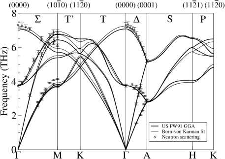
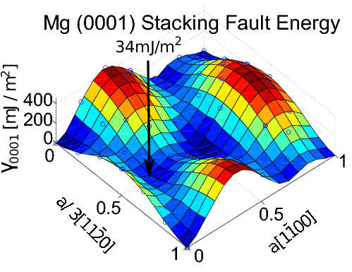
Figure 1: First-principles phonon spectra (top) and $(0001)$ generalized stacking-fault energy (bottom) for Mg. These describe response of the lattice to small displacements, elastic deformation, and slip in the basal plane. Density-functional theory is able to accurately reproduce the vibrational spectra from experimental measurements: Neutron scattering data from [14], and a Born-von Karman fit to the data from [15]. The equilibrium lattice constants from the ultrasoft pseudopotential are $a=3.19\text{\AA}$ and $c=5.18\text{\AA}$; the elastic constants, which determine the slopes of the spectra for long wavelengths are $C_{11}=60\text{GPa}$, $C_{33}=61\text{GPa}$, $C_{12}=21\text{GPa}$, $C_{13}=20\text{GPa}$, and $C_{44}=18\text{GPa}$. For the generalized-stacking fault surface, a single plane of Mg is displaced in the basal plane by a linear combination of $\frac{a}{3}[11\bar{2}0]$ and $a[1\bar{1}00]$; the defected geometry is allowed to relax in the $[0001]$ directions, and the energy per area for the defect is the generalized stacking-fault energy. The highlighted point of $\frac{a}{3}[10\bar{1}0]$ is a metastable configuration known as the intrinsic I2 stacking fault. The $\gamma_{\text{I2}}$ energy agrees well with other density-functional theory calculations of the same[16]. The I2 stacking fault geometry is the basis for computing chemical misfits for solutes.

Efficient computation of interactions between solutes and dislocations requires simulation cells and flexible boundary condition approaches that isolate individual defects. Calculations are performed with VASP[2, 3], a plane-wave density-functional theory code. Magnesium and all solutes are treated with Vanderbilt ultrasoft pseudopotentials[5, 6], and the Perdew-Wang 91 GGA exchange-correlation potential[4]. The ultrasoft Mg pseudopotential ([Ne]$3s^{2}$) accurately reproduces experimental lattice[17] (less than 0.9% error) and elastic[18] (less than 5% error) constants, and phonon frequencies[14, 15] (less than 3% error) of bulk Mg; c.f. Figure 1. The stacking-fault surface in Figure 1, while not available experimentally, compares well with other density-functional theory calculations[16]. We chose a planewave cutoff of 138eV, $k$-point meshes (see below for specific values tied to each geometry) and Methfessel-Paxton smearing of 0.5eV to give an energy accuracy of 5meV for bulk Mg. For calculations involving solutes, the cutoff energy was increased as necessary to accommodate harder pseudopotentials for solutes; c.f. Table 2 for all cutoff energies used for the corresponding pseudopotentials (in general, we selected a cutoff energy of 1.3 times the suggested cutoff for the potential). The geometries for misfits, and dislocation calculations and coupling with lattice Green function flexible boundary condition methods are given below.

2.1 Size misfit

For the size misfit, we substituted single solutes into a $2\times 2\times 2$ Mg supercell ($k$-point mesh of $16\times 16\times 10$) at five different volumes based on the equilibrium Mg volume $V_{0}$: $1.16V_{0}$, $1.05V_{0}$, $1.00V_{0}$, $0.95V_{0}$, $0.86V_{0}$. The atomic positions in each supercell were relaxed until all forces were less than 5meV/Å. The size misfit is the logarithmic derivative of the Burgers vector $b=\frac{a}{3}[2\bar{1}10]$ with solute concentration $c_{\text{s}}$ in the dilute limit; hence,

$$\varepsilon_{b}=\left.\frac{d\ln b}{dc_{\text{s}}}\right|_{c_{\text{s}}=0}=\frac{1}{b}\left.\frac{db}{dc_{\text{s}}}\right|_{c_{\text{s}}=0}.$$ (1)

The change in energy for a solute with volume is given by the differences in supercell energies $E_{\text{solute supercell}}(e_{V})-E_{\text{solute supercell}}(0)-15E_{\text{bulk Mg}}(e_{V})+15E_{\text{bulk Mg}}(0)$ and varies with the volumetric strain $e_{V}=V/V_{0}-1$ for each supercell. The raw data is fit to a quadratic in strain $E^{\prime}_{\text{solute}}e_{V}+E^{\prime\prime}_{\text{solute}}e_{V}^{2}$, and the slope $E^{\prime}$ is used to determine the size misfit

$$\varepsilon_{b}=-\frac{E^{\prime}}{3BV_{0}},$$ (2)

where $B$ is the bulk modulus. We use the slope $E^{\prime}_{\text{solute}}$ to compute the change in binding energy for a solute due to local volumetric strain. Comparison with calculations using a larger $3\times 3\times 3$ supercell affected the size misfit by $\lesssim 10\%$.

2.2 Chemical misfit

For the chemical misfit, we substituted single solutes into a $2\times 2\times 9$ Mg supercell ($k$-point mesh of $16\times 16\times 1$) corresponding to 18 $(0002)$ planes. The supercell vector along the $c[0001]$ direction has an extra $\frac{a}{3}[01\bar{1}0]$ component, so that the supercell represents a periodic repetition of stable stacking faults separated by a distance of $9c$. The solute is substituted into a site in the stacking fault, and the atomic positions were relaxed until forces were less than 5meV/Å. Because the I2 intrinsic stacking-fault configuration is (meta)stable (c.f. Figure 1), we do not impose any constraints on the relaxation. The chemical misfit is the logarithmic derivative of the I2 intrinsic stacking-fault energy $\gamma_{\text{I2}}$ with solute concentration $c_{\text{s}}$ in the dilute limit; hence,

$$\varepsilon_{\text{SFE}}=\left.\frac{d\ln\gamma_{\text{I2}}}{dc_{\text{s}}}\right|_{c_{\text{s}}=0}=\frac{1}{\gamma_{\text{I2}}}\left.\frac{d\gamma_{\text{I2}}}{dc_{\text{s}}}\right|_{c_{\text{s}}=0}.$$ (3)

The chemical misfit is calculated from our supercell energies as

$$\varepsilon_{\text{SFE}}=\frac{E_{\text{displaced}}(\text{solute})-E_{\text{undisplaced}}(\text{solute})-2\sqrt{3}a^{2}\gamma_{\text{I2}}}{\gamma_{\text{I2}}\sqrt{3}a^{2}/2},$$ (4)

where the “displaced” and “undisplaced” geometries correspond to the layered structure with and without an I2 intrinsic stacking fault, and $\sqrt{3}a^{2}/2$ is the basal plane area.

2.3 Dislocation geometries

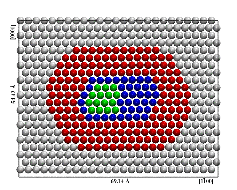
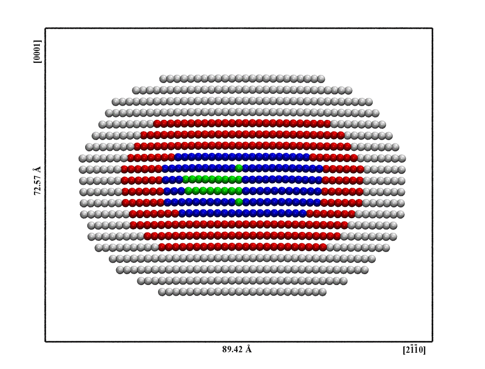
Figure 2: Full Mg basal screw (top) and edge (bottom) dislocation core equilibrium geometries, separated into regions I (blue), II (red), and III (gray) and identified solute sites (green). The periodic simulation boxes are $69.14\times 54.42\times 3.19$ ų for screw and $84.92\times 72.57\times 5.53$ ų for edge. The initial screw geometry has displacements coming out of the page, while the edge displacements are in the plane of the page; relaxation produces additional displacements in the core of the partial dislocations.

Flexible boundary condition methods[19, 7, 8] relax the pure Mg basal dislocation geometries. The starting geometry comes from the anisotropic elasticity solution for a dislocation using the elastic and lattice constants from our first principles calculations [20, 21]. The elasticity solution determines the displacement field as a continuum function; we start with a bulk HCP lattice periodically repeated along the dislocation line direction: $\frac{a}{3}[2\bar{1}\bar{1}0]$ for the screw ($k$-point mesh of $1\times 1\times 16$) and $a[01\bar{1}0]$ for the edge ($k$-point mesh of $1\times 1\times 12$). The displacement field is centered between two $(0002)$ atomic planes, and applied to every atom. A finite sized computational cell is produced by simulating only atoms within 10 lattice planes from the estimated positions of the partial cores; c.f. Figure 2. The distance from the core is determined by summing the distance to return to small relative displacements (the size of region I), the distance for the lattice Green function to match the elastic Green function[8] (the size of region II), and the distance from an unrelaxed free surface to produce zero forces (the size of region III). Together, this ensures that region II both does not have spurious forces due to the vacuum outside and is sufficiently separated from the defect core to follow the bulk harmonic response. In the case of the screw dislocation, the lack of a long-range volumetric strain field allows the use of a periodic simulation cell with “domain boundaries” at the cell boundaries. For the edge dislocation, vacuum is needed to isolate periodic images of the dislocations.

2.4 Flexible boundary conditions

Lattice Green function-based flexible boundary conditions isolate the dislocation at the center of the simulation cell from the domain boundaries or vacuum while displacing surrounding atoms as if the dislocation were embedded in infinite bulk responding harmonically[19, 7]. The method relaxes each atom based on its location within one of three different regions determined by the distance from the dislocation core. Overall, the screw dislocation consists of 525 atoms and the edge dislocation consists 806 atoms. Region I atoms near the core (54 for the screw, 130 for the edge) start the simulation with non-zero forces, and are relaxed using a conjugate-gradient method. As the relaxation commences, the neighboring atoms in region II (164 for the screw, 247 for the edge) start with zero forces but the forces increase as atoms in region I are displaced. The region II atoms can be treated as if they were coupled to infinite harmonic bulk; hence, their forces can be relaxed by applying a displacement to each atom $\vec{R}$ given by the lattice Green function (LGF): $\vec{u}(\vec{R})=\sum_{\vec{R}^{\prime}}{\bf G}(\vec{R}-\vec{R}^{\prime})\vec{f}(\vec{R}^{\prime})$, where $\vec{R}^{\prime}$ only varies over atoms in region II, $\vec{f}$ are their forces, and ${\bf G}(\vec{R}-\vec{R}^{\prime})$ is the (tensor) LGF. This displaces all atoms—including region I atoms, and the outer region III atoms (307 for the screw, and 429 for the edge). The atoms in the outer region have non-zero forces due to the domain boundary or vacuum; but the lattice Green function displaces them as if they were part of an infinite bulk lattice. The relaxation cycle continues between region I (conjugate gradient) and II (lattice Green function) until the forces are less than 5meV/Å in both regions. The final result of the relaxation is the stress-free dislocation core equilibrium geometry.

2.5 Direct solute-dislocation interaction energy calculation

We compute the interaction of Al with Mg dislocations by direct substitution of Al for Mg at different sites in the dislocation cores; c.f. Figure 2. For each substitution, the entire region I was relaxed until the forces were less than 5meV/Å. This defines the relative energies for Al in each site (18 for the screw, 30 for the edge); to define the energy zero for Al—the reference of Al substituted into bulk Mg with no strain field—we reference the average energy of Al above and below the stacking fault region. The periodic repetition of the solute along the dislocation line introduces a finite-size error in the calculated solute-dislocation interaction. For the screw dislocation geometry, there is one Al atom every 3.19Å along the dislocation line, and for the edge dislocation, every 5.53Å. Using a screw dislocation geometry with double the periodicity (6.38Å), the calculated Al solute/screw dislocation interaction energy was 8.4meV higher than that extracted from the original geometry. We expect this to be an upper limit on the finite-size error as it is (a) for the shortest Al-Al repeat distance, and (b) for the largest change in local geometry.

2.6 Misfit approximation of solute-dislocation interaction energy

To compute the interaction of any solute with the Mg dislocations, we analyzed each dislocation geometry in terms of local volumetric strain and slip. The local volumetric strain at each atomic site in the final relaxed dislocation geometry is defined from the nearest-neighbor positions as

$$e_{V}=\left[\frac{\det\left\{\sum_{\vec{x}^{\prime}}x^{\prime}_{i}x^{\prime}_{j}\right\}}{\det\left\{\sum_{\vec{x}}x_{i}x_{j}\right\}}\right]^{1/2}-1$$ (5)

where $\vec{x}^{\prime}$ are the vectors to nearest neighbors for a site, and $\vec{x}$ are the corresponding nearest-neighbor vectors in the HCP lattice[22]. The slip interaction energy ($E_{\text{slip}}$) is calculated at each atomic site as

$$E_{\text{slip}}=\frac{\sqrt{3}a^{2}/2}{6}\sum_{\vec{d}}\gamma_{(0001)}\left(\vec{d}\right),$$ (6)

where $\vec{d}$ are the vectors to the nearest neighbors in adjacent basal planes, $\gamma_{(0001)}$ is the generalized basal stacking-fault energy for displacement $\vec{d}$, and the factor of $\frac{1}{6}$ is from assigning half the bond energy for the 3 out-of-plane neighbors. The interaction energy for a solute is then a sum of two contributions: the size interaction (given by the change in solute energy at the site strain) and slip interaction (given by the chemical misfit multiplied by the slip energy of the site)

$$\begin{split}E_{\text{binding}}&=E^{\prime}_{\text{solute}}e_{V}+E_{\text{slip}}\cdot\varepsilon_{\text{SFE}}\\ &=-3BV_{0}\cdot e_{V}\cdot\varepsilon_{b}+E_{\text{slip}}\cdot\varepsilon_{\text{SFE}}.\end{split}$$ (7)

This misfit approximation requires significantly less computing resources to determine compared with direct calculations.

3 Dislocation / solute interactions

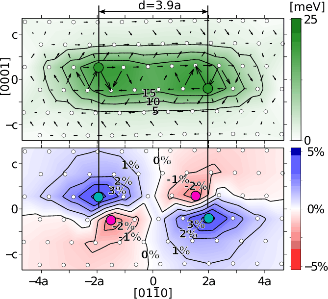
Figure 3: Mg basal screw dislocation core geometry with atomically resolved slip energy (top) and volumetric strain (bottom). The equilibrium geometry is found using first-principles flexible boundary condition methods. The circles show positions of atomic rows repeated out of the page (the $[2\bar{1}\bar{1}0]$ direction), while the magnitude of arrows between neighboring sites represent the relative displacement of the neighboring rows out of the page. The arrow magnitude is maximum for the partial slip. The dislocation splits into two partials—whose cores are centered on a closed circuit of arrows—with screw components (displacements out of the page) of $0.5a$, and edge components (displacements in the horizontal slip plane) of $0.289a$, separated by $3.9a$. The slip energy is computed from the atomic geometry based on the relative displacements of neighbors, and has a maximum value of 20meV at the green sites. The volumetric strain is computed from the average change in nearest neighbor distances, and has a maximum tensile value of $+4.6\%$ at the cyan sites and maximum compressive value of $-2.7\%$ at the magenta sites.

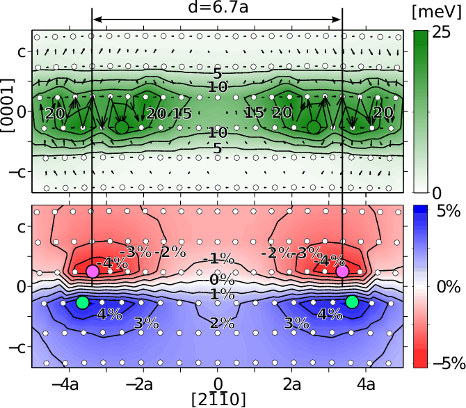
Figure 4: Mg basal edge dislocation core geometry with atomically resolved slip energy (top) and volumetric strain (bottom). The equilibrium geometry is found using first-principles flexible boundary condition methods. The circles show positions of atomic rows repeated out of the page (the $[01\bar{1}0]$ direction), while the magnitude of arrows between neighboring sites represent the relative displacement of the neighboring rows along the horizontal slip plane. The arrow magnitude is maximum for the partial slip. The dislocation splits into two partials—whose cores are centered on a closed circuit of arrows—with edge components (displacements in the horizontal slip plane) of $0.5a$, and screw components (displacements out of the page) of $0.289a$, separated by $6.7a$. The slip energy is computed from the atomic geometry based on the relative displacements of neighbors, and has a maximum value of 25meV at the green sites. The volumetric strain is computed from the average change in nearest neighbor distances, and has a maximum tensile value of $+5.3\%$ at the cyan sites and maximum compressive value of $-4.9\%$ at the magenta sites.

Figure 3 and Figure 4 show the first-principles equilibrium basal screw and edge dislocation core geometries analyzed in terms of size and slip at each atomic site. The screw dislocation has displacements (slip) parallel to the line direction (out of the page), and the edge dislocation has slip perpendicular to the line direction, representing the two limiting cases for basal dislocation geometry. The equilibrium screw dislocation geometry dissociates into $\frac{a}{3}[10\bar{1}0]$ and $\frac{a}{3}[01\bar{1}0]$ partial dislocations separated by $3.9a$ of I2 stacking fault, where $a$ is the basal lattice spacing. The equilibrium edge dislocation also dissociates into partial dislocations (half the slip of the full dislocation), separated by $6.7a$ of stacking fault. The “cores” of the partials have the largest change in local geometry from bond-stretching and bond-bending. For a screw dislocation, there is no far-field dilation (tension or compression); however, we find a large volumetric strain in the partial cores. The strain is comparable to that in the edge dislocation core, which does have a far-field dilation strain. We quantify the bond-bending with the relative displacement $\vec{d}$ of each atomic row, and average the energy of stacking faults with displacement $\vec{d}$ of the six neighbors to give a slip energy $E_{\text{slip}}$. This energy is localized to the partial cores and the stacking fault separating them. A solute’s binding energy will change in the dislocations due to the different local geometry; moreover, as the cores show the greatest change in local environment, we expect solutes to provide the strongest interactions from sites within the dislocation cores.

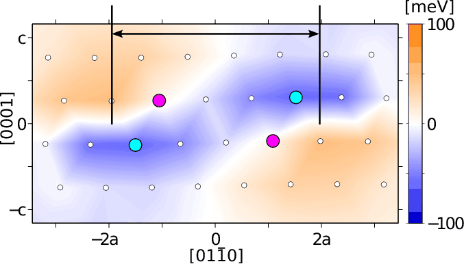
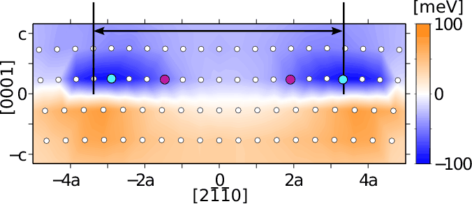
Figure 5: Al interaction energies with Mg screw (top) and edge (bottom) dislocations, from first principles. We substitute Al atoms at different sites in and around the partial cores, and compute the energy differences after relaxation. The cyan sites show points of maximum binding energy while the magenta sites show maximum interaction force—i.e., greatest change in binding energy along the slip plane (c.f. Table 1 for numerical values). The sites between the partial cores and stacking faults have the largest interaction force for both dislocation types. The strong Al interaction with the screw dislocation is surprising, and can only be accurately resolved through the atomic-scale calculation of the full dislocation core geometry.

Figure 5 shows the first-principles interaction energy—the change in the solute binding energy—for an Al solute with screw and edge dislocation cores. We find the strongest interaction at the site of maximum compression near the center of the dislocation partial cores for both the edge and the screw geometries. We expect this, since Al is smaller than Mg and is affected by the size changes in the core. The interaction force (the derivative of the interaction energy in the slip direction) is largest between the partial cores and the stacking fault for both dislocations, with nearly equal magnitudes for edge and screw. The similar values for the screw and edge forces are surprising as elasticity theory predicts a very weak far-field interaction for the screw dislocation[12]. If we apply anisotropic elasticity theory at a distance of $c/4$ from the slip plane (where $c/2$ is the distance between parallel basal slip planes) to the screw and edge dislocations separated into mixed partials ($\frac{a}{3}[1\bar{1}00]$ and $\frac{a}{3}[10\bar{1}0]$), anisotropic elasticity theory predicts maximum and minimum volumetric strains in the partial cores of $\pm 7.2\%$ (screw) and $\pm 12.7\%$ (edge). This is significantly different from our atomic-scale values of –2.7%, +4.6% (screw) and –4.9%, +5.3% (edge). Moreover, elasticity theory predicts the maximum interaction forces for solutes to be the maximum interaction energy divided by 2Å, and that the solute/screw interaction force will be $58\%$ of the solute/edge interaction force. All of the elasticity predictions contradict our atomic-scale calculations: equal solute/screw and solute/edge interaction forces, energy to force ratios of 6–8Å, and smaller and unbalanced maximum and minimum volumetric strains. All of these differences highlight the sensitivity of the solute-dislocation interaction to the partial core geometries and the need for a first-principles approach to compute stress-free atomic-scale dislocation core geometries.

We replace the elasticity approach to solute-dislocation interaction with a fully atomic-scale approach based on size and chemical misfits. The long-range strain and stress fields of a dislocation are known from anisotropic elasticity[21], and so the change in local volume around a solute (size misfit $\varepsilon_{b}$, the logarithmic derivative of the lattice constant with solute concentration) controls the solute-dislocation interaction. In the dislocation core, the interaction energy is largest, but it is no longer described by elasticity. Despite this, we can use the size misfit even in the partial cores by computing the change in local volume for each atomic site. This approximation is the largest contribution to the interaction energy; the next largest contribution is from the slip in the partial cores and the stacking fault. In the same way that we determine a slip energy in the core of the dislocation, we find that solutes change the response of the crystal to slip (chemical misfit $\varepsilon_{\text{SFE}}$, the logarithmic derivative of the stacking-fault energy with solute concentration). The chemical misfit determines how the atomically-resolved slip energy (c.f., Figure 3 and Figure 4) will change with the addition of a solute. Adding this contribution to the size misfit produces an accurate approximation of the solute-dislocation interaction energy using the dislocation core geometry.

Table 1: Al interaction energy with Mg basal screw and edge dislocations from direct solute substitution calculations (c.f. Figure 5) and misfit approximations based on the dislocation geometry. The maximum binding energy (meV) and maximum interaction force (meV/Å) determine the attraction of solutes to dislocations and solid-solution strengthening. The misfit approximation uses two misfits with the atomic-scale dislocation geometry: change in local volume, and bond-bending from slip to compute interaction energies for solute with the dislocation core. For both dislocation geometries, the misfit approximation correctly captures the interaction energies and forces compared with the more computationally intensive direct calculation.

screw	$E_{\text{binding}}$	$F_{\text{max}}$
direct (Figure 5)	60	11.4
misfit: volume	46	12.6
misfit: volume + slip	65	11.2
edge	$E_{\text{binding}}$	$F_{\text{max}}$
direct (Figure 5)	99	12.2
misfit: volume	81	11.6
misfit: volume + slip	105	11.5

Table 1 compares the solute-dislocation interaction for Al computed using direct substitution into the dislocation cores with our combined size and chemical misfit approach. The response of Al to changes in local volume and slip capture most of the interaction energy and forces in the dislocation core. Moreover, the strain and slip energies are taken directly from the equilibrium core geometries, and the size and chemical misfit calculations include the local response of Mg atoms neighboring the Al solute. The size-misfit approximation is expected to be accurate in the far-field, and is accurate even in the partial cores where the interaction is the strongest. The slip energy is needed to represent the stacking fault region between the partials, and the center of the partial cores themselves. The maximum interaction forces from the misfit calculation are accurate to within 5% of the direct calculations for both screw and edge geometries, with deviations of only 5meV for the interaction energies; hence, we can predict the interaction energies of other solutes by using the size and chemical misfits combined with the equilibrium dislocation core geometries. This permits us to use much simpler and computationally efficient first-principles calculations of misfits with our first-principles calculation of pure Mg dislocation cores.

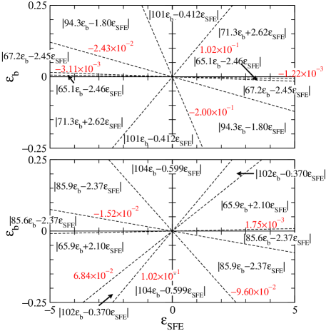
Figure 6: Formulae for computation of maximum solute-dislocation interaction forces from $\varepsilon_{b}$ and $\varepsilon_{\text{SFE}}$ for edge (top) and screw (bottom) dislocations. Each solute substitutional site in the screw or edge dislocation has a local volumetric strain and slip energy; we use the size and chemical misfits to approximate the solute-dislocation interaction energy by linearly scaling those energies. The derivative of the solute-dislocation interaction energy along the slip direction gives the interaction force, and the maximum interaction force appears as input in our strengthening model (Equation 10). The particular site that produces the largest interaction force changes depending on the magnitudes of the misfits $\varepsilon_{b}$ and $\varepsilon_{\text{SFE}}$, leading to different regimes. The slopes of the lines separating the different regimes are indicated in red.

Figure 6 provides the formulae for the maximum solute-dislocation interaction force in terms of misfits. The interaction force from the first-principles solute binding energy is $F_{\text{max}}=\max|\hat{m}\cdot\nabla E_{\text{binding}}|$ where $\hat{m}$ is the dislocation slip direction ($[1\bar{1}00]$ for screw and $[11\bar{2}0]$ for edge), and $E_{\text{binding}}$ is the sum of the solute slip and size interaction energies from Equation 7. The gradients of the solute size and slip interactions are calculated as a centered difference in the slip direction for sites near the partial dislocation cores where the gradient is the largest. The gradients were scaled by the size and chemical misfits for each solute and summed to determine the maximum interaction force. The end result is that, for any combination of $\varepsilon_{b}$ and $\varepsilon_{\text{SFE}}$, the strongest interaction force site is known, and its pinning force can be computed as a linear combination of the two parameter; however, the coefficients change as different magnitudes of $\varepsilon_{b}$ and $\varepsilon_{\text{SFE}}$ will select different sites as the strongest interaction force site. Figure 6 graphically summarizes all of the formulae for each range of $\varepsilon_{b}$ and $\varepsilon_{\text{SFE}}$. For example, Al has $\varepsilon_{b}=-0.115$ and $\varepsilon_{\text{SFE}}=-1.252$; then, for the edge dislocation, the interaction force is given by the formula in the southwest corner $|71.3\varepsilon_{b}+2.62\varepsilon_{\text{SFE}}|=11.5\text{meV/\AA}$, and for the screw dislocation, the interaction force is given by the formula in the narrow southwest wedge $|102\varepsilon_{b}-0.370\varepsilon_{\text{SFE}}|=11.2\text{meV/\AA}$. For Zn, $\varepsilon_{b}=-0.153$ and $\varepsilon_{\text{SFE}}=+0.317$, so the edge dislocation interaction force is given by the formula in the south section $|101\varepsilon_{b}-0.412\varepsilon_{\text{SFE}}|=15.6\text{meV/\AA}$ and for the screw dislocation, the interaction force is given by the formula in the south section $|104\varepsilon_{b}-0.599\varepsilon_{\text{SFE}}|=16.1\text{meV/\AA}$.

4 Solid-solution strengthening model

To predict solid-solution strengthening, we use our first-principles atomic-scale solute-dislocation interaction calculation as input to a dilute-concentration, weak-obstacle model for solid-solution strengthening from Fleischer[23]. As the dislocation moves in the slip plane under stress, it encounters randomly placed immobile solute atoms each of which provides a “pinning” force up to the maximum solute-dislocation interaction force $F_{\text{max}}$. This point-pinning model is applicable for isolated obstacles with a short-ranged—on the scale of the solute-separation distance—interaction force between solute and dislocations, and hence will capture the dilute-concentration limit. It also assumes a random solute distribution that does not rearrange due to the dislocation strain-fields; hence, it is operable at temperatures where no appreciable solute diffusion occurs. The nearly straight dislocation bows at the solute until it reaches a critical bowing angle $\theta_{c}$ and the line tension $\mathcal{E}$ pulls the dislocation past the solute. At the critical angle $\theta_{c}$, $F_{\text{max}}=2\mathcal{E}\sin((\pi-\theta_{c})/2)$. For weak obstacles, the dislocation is nearly straight, and the critical bowing angle is only slightly smaller than $\pi$, hence $\pi-\theta_{c}\approx F_{\text{max}}/\mathcal{E}\ll 1$. The mean distance between pinning points, $L$, is the average distance between nearest randomly placed solutes in a circular wedge of angle $\alpha=(\pi-\theta_{c})/2$, where $L=\sqrt{\pi/(2\rho_{s}\alpha)}$, and $\rho_{s}$ is the density of solutes in the slip plane. The solute density is $2c_{\text{s}}$ (atomic concentration $c_{\text{s}}$) per $\sqrt{3}b^{2}/2$ (Burgers vector $b=a$, basal lattice constant), assuming that the solute can appear either above or below the slip plane; hence,

$$L=\left(\frac{\pi}{\rho_{s}(\pi-\theta_{c})}\right)^{1/2}=\left(\frac{\pi\sqrt{3}b^{2}}{4(\pi-\theta_{c})c_{\text{s}}}\right)^{1/2}=\frac{(3\pi^{2})^{1/4}b}{2}\left(\frac{\mathcal{E}}{F_{\text{max}}}\right)^{1/2}c_{\text{s}}^{-1/2}.$$ (8)

That is, the distance between pinning points increases with decreasing solute concentration $c_{\text{s}}$ and with decreasing interaction force. Given the mean solute spacing, the strengthening (increase in critical-resolved shear stress in the basal plane necessary to overcome the solute restraining force) is:

$$\Delta\tau_{\text{CRSS}(0001)}=\frac{F_{\text{max}}}{bL}=\frac{2}{(3\pi^{2})^{1/4}}\frac{\mathcal{E}}{b^{2}}\left(\frac{F_{\text{max}}}{\mathcal{E}}\right)^{3/2}\sqrt{c_{\text{s}}},$$ (9)

which scales as $F_{\text{max}}^{3/2}$ and $\sqrt{c_{\text{s}}}$. This is the change for a (nearly) straight dislocation line of a given character ranging from edge to screw; the interaction energy and line tension correspond to the particular line orientation. The strengthening of an average dislocation loop—which continuously ranges from edge to screw orientations—is weighted by the line tension. The shape of a basal loop can be estimated as an ellipse with axial ratio $\alpha=K_{e}/K_{s}$, where $K_{e}=25.6\text{GPa}$ and $K_{s}=18.6\text{GPa}$ are the edge and screw line energy prefactors[20] as determined from the first-principles elastic constants $C_{ij}$. For Mg, this gives a weight of 0.539 for the screw dislocation and 0.461 for the edge. The screw and edge line tensions are $\mathcal{E}_{s}=\frac{1}{2}K_{s}b^{2}=591\text{meV/\AA}$ and $\mathcal{E}_{e}=\frac{1}{2}K_{e}b^{2}=817\text{meV/\AA}$; so, the dislocation loop weighted-average strengthening for each solute is

$$\Delta\tau_{\text{CRSS}(0001)}=\left[0.30\Big{(}F^{\text{screw}}_{\text{max}}\Big{)}^{3/2}+0.22\Big{(}F^{\text{edge}}_{\text{max}}\Big{)}^{3/2}\right]\cdot c_{\text{s}}^{1/2},$$ (10)

where $\Delta\tau_{\text{CRSS}(0001)}$ is in MPa and the interaction forces are in meV/Å.

Hence we need to consider the contributions to strength from both edge and screw dislocations for all solutes in our modified-Fleischer model. The concentration-independent prefactor in Equation 10 is the solute “strengthening potency.” The solubility of a solute controls the maximum possible $\sqrt{c_{\text{s}}}$, and hence the maximum possible strengthening of a solute in an alloy. Combining the calculation of interaction strengths from their misfits, the strength potency can be fit to an approximate functional form

$$\Delta\tau_{\text{CRSS}(0001)}\approx(38.9\text{MPa})\left\{\left(\frac{\varepsilon_{b}}{0.176}\right)^{2}+\left(\frac{\varepsilon_{\text{SFE}}}{5.67}\right)^{2}-\frac{\varepsilon_{b}\varepsilon_{\text{SFE}}}{2.98}\right\}^{3/2}\cdot c_{\text{s}}^{1/2}.$$ (11)

The negative $\varepsilon_{b}\varepsilon_{\text{SFE}}$ term shows that the effect of the size and chemical misfits is not completely independent, but that due to the geometry of the dislocation core—where the sites of largest slip energy are neighboring sites of largest strain energy—a larger gradient can be produced by having the size and slip misfits with opposite signs. However, the magnitude of the denominators also shows that the size misfit is the dominant interaction. The fit had a maximum error of 10%, with the average error being 3%. As this model ignores thermally activated processes to overcome solute obstacles, it is appropriate at temperatures without appreciable diffusion, but the fundamental interaction data is usable for high temperature strengthening models as well. All of the material information that enters Equation 10 comes completely from first principles: crystal structure, lattice and elastic constants, dislocation core geometries, and solute misfits.

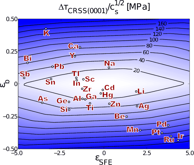
Figure 7: Solid-solution strengthening potency (contours) versus their size ($\varepsilon_{b}$) and chemical ($\varepsilon_{\text{SFE}}$) misfits for 29 different solutes in Mg. The misfits, combined with the screw and edge dislocation geometries (c.f. Figure 3 and Figure 4) determine the maximum interaction forces. In the dilute limit for weak obstacles, the strengthening—characterized by a change in the basal critical-resolved shear stress $\Delta\tau_{\text{CRSS}(0001)}$—scales with $\sqrt{c_{\text{s}}}$ and with the interaction forces to the 3/2 power in Equation 10. We can efficiently predict the solute strengthening for a whole range of solutes from the first-principles core geometry. This “design map” shows solutes with comparable strengthening potency, and also gives a guide to solubility—which decreases with increasing misfit magnitudes.

Figure 7 combines the first-principles data for size and chemical misfits with the simple solid-solution strengthening model of Equation 10 into a “design map” for the strengthening potencies of 29 different solutes. The contours show equal strengthening potency versus size and chemical misfits. The size and chemical misfits can be easily computed for any substitutional solute in the periodic table, and then the screw and edge dislocation maximum interaction forces to predict the change in critical-resolved shear stress for basal slip from Equation 10. This map provides a rational method to select equipotent solutes to replace less “desirable” elements based on high mass, cost, or other processing concerns. In addition, the misfits also give rough qualitative information about solubility, as larger misfit magnitudes lead to lower solubilities. For example, for Zn with a potency $\Delta\tau_{\text{CRSS}(0001)}/\sqrt{c_{\text{s}}}=32.5\text{MPa}$, the corresponding small magnitudes of $\varepsilon_{b}$ and $\varepsilon_{\text{SFE}}$ suggest a high solubility. Alternatively, the much larger potencies of Ir (172MPa) and K (161MPa) are due to the larger magnitudes of $\varepsilon_{b}$ and $\varepsilon_{\text{SFE}}$, giving rise to a much lower solubility. Yttrium represents a reasonable compromise between strength and solubility.

Table 2: Substitutional solutes with pseudopotential valence configuration and energy cutoff, size and chemical misfits, corresponding maximum interaction force with an edge and screw dislocation, and computed interaction forces from Figure 6 and strengthening potency from Equation 10, and from single crystal, low temperature, dilute-concentration experimental measurements where available. In the case of Bi and Pb, low concentration data is not available; instead plateau stress (potency at higher concentration) serves as a lower limit on the dilute-concentration potency.

					F${}_{\text{max}}$ (meV/Å)		potency (MPa)
solute	USPP cutoff (eV)		$\varepsilon_{b}$	$\varepsilon_{\text{SFE}}$	edge	screw	eqn.10	exper.
Ag	[Kr]$4d^{10}5s^{1}$	235	–17.1%	1.93	19.6	19.3	44.1
Al	[Ne]$3s^{2}3p^{1}$	168	–11.5%	–1.25	11.5	11.2	19.6	21.2 [24]
As	([Ar]$3d^{10}$)$4s^{2}4p^{3}$	188	–14.5%	–3.60	19.8	17.1	40.3
Be	[He]$2s^{2}$	327	–25.2%	1.33	26.1	27.1	71.1
Bi	([Xe]$4f^{14}5d^{10}$)$6s^{2}6p^{3}$	138	16.2%	–4.45	23.3	24.5	60.6	$>25.0$ [24]
Ca	[Ar]$4s^{2}$	138	28.2%	–1.39	29.1	30.3	83.8
Cd	[Kr]$4d^{10}5s^{2}$	218	–4.6%	–0.06	4.6	4.8	5.3	6.0 [25]
Ga	([Ar]$3d^{10}$)$4s^{2}4p^{1}$	169	–11.9%	–1.09	11.6	11.8	20.7
Ge	([Ar]$3d^{10}$)$4s^{2}4p^{2}$	181	–13.9%	–2.04	15.2	13.4	27.6
Hg	([Xe]$4f^{14}$)$5d^{10}6s^{2}$	207	–7.3%	–0.18	7.3	7.5	10.5
In	([Kr]$4d^{10}$)$5s^{2}5p^{1}$	138	2.8%	–1.58	5.8	6.2	7.6	9.0 [24]
Ir	([Xe]$4f^{14}$)$5d^{7}6s^{1}$	258	–43.5%	4.33	48.8	48.0	173.1
K	[Ar]$4s^{1}$	138	42.5%	–3.38	46.2	46.4	162.5
Li	[He]$2s^{1}$	138	–5.8%	1.89	8.9	9.4	14.4	11.2 [26]
Mn	[Ar]$3d^{6}4s^{1}$	295	–35.6%	2.12	37.4	38.5	120.8
Na	[Ne]$3s^{1}$	138	12.6%	0.29	12.6	12.9	23.6
Pb	([Xe]$4f^{14}5d^{10}$)$6s^{2}6p^{2}$	138	13.2%	–3.00	17.9	18.5	40.1	$>14.0$ [24]
Pd	[Kr]$4d^{9}5s^{1}$	259	–31.8%	3.75	36.7	36.2	113.5
Pt	([Xe]$4f^{14}$)$5d^{9}6s^{1}$	249	–37.7%	3.39	41.6	41.3	137.5
Ru	[Kr]$4d^{7}5s^{1}$	265	–40.1%	3.92	44.9	44.2	153.0
Sb	([Kr]$4d^{10}$)$5s^{2}5p^{3}$	139	4.6%	–4.65	14.5	15.0	29.3
Sc	[Ar]$3d^{2}4s^{1}$	195	3.5%	–1.20	5.5	5.9	7.0
Si	[Ne]$3s^{2}3p^{2}$	196	–19.9%	–2.03	19.5	19.6	44.5
Sn	([Kr]$4d^{10}$)$5s^{2}5p^{2}$	138	3.7%	–3.08	10.1	10.5	17.1	24.3 [27]
Ti	[Ar]$3d^{3}4s^{1}$	236	–14.9%	–0.81	14.8	15.1	29.8
Tl	([Xe]$4f^{14}$)$5d^{10}6s^{2}6p^{1}$	231	4.7%	–1.61	7.3	7.8	10.8	8.2 [28]
Y	[Kr]$4d^{2}5s^{1}$	155	21.2%	–1.70	23.1	23.2	57.3
Zn	[Ar]$4s^{2}3d^{10}$	272	–15.3%	0.32	15.6	16.1	32.7	31 [29]
Zr	[Kr]$4d^{3}5s^{1}$	195	–3.8%	–1.27	6.0	5.1	6.7

Table 2 provides misfits and potencies for all 29 solutes, as well as comparisons to available experimental data (for Al, Zn, Bi, Cd, In, Li, Pb, Sn, and Tl). For comparison, we look to single-crystal, low temperature measurements of critical resolved shear stress of Mg in the low concentration limit. For example, the available experimental data for potencies of common solutes Al and Zn in Mg extrapolated to 0K[24, 29] give 21.2MPa and 31MPa, versus our first-principles prediction of 19.5MPa and 32.5MPa—validating our computation and modeling approach. For Bi and Pb, only plateau stress data is available—this is the strengthening divided by $\sqrt{c_{\text{s}}}$ at larger concentrations than considered here. We expect the plateau strengthening coefficient to be a lower limit on our dilute concentration potency, and so our data remains consistent with the available experimental data.

5 Conclusions

The basal-slip strengthening design map for Mg represents an important development in predicting chemical effects on strengthening in an accurate and efficient manner. In addition to predicting strength, we find a strong solute interaction with screw dislocations equal to that of edge dislocations: this demonstrates the need for first-principles quantum-mechanical calculations with flexible boundary conditions to reveal defect interactions. Maximizing strength requires careful consideration of the important tradeoff between high strengthening capacity (i.e., large solute misfits) and high solubility (low misfit magnitudes). Predicting strength above dilute concentrations, at higher temperatures and including other mechanisms such as forest strengthening[30] will require the fundamental input from the present solute strengthening predictions. Moreover, cross-slip in Mg depends on the constriction of basal screw dislocations, and should be aided by solutes with positive $\varepsilon_{\text{SFE}}$ to increase the basal stacking-fault energy. By finding solutes that can improve cross-slip while simultaneously strengthening basal slip—as approached here—the strength anisotropy of Mg alloys can be reduced, improving ductility. The natural extension of the computational methodology developed herein is to predict solute effects on slip in prismatic planes, including increasing cross-slip for ductility enhancement. In addition, atomically-resolved strengthening predictions hold great promise for the design of other technologically important HCP metals such as Ti and Zr.

Acknowledgments

The authors thanks W. A. Curtin for helpful discussions. This research was sponsored by NSF through the GOALI program, Grant 0825961, and with the support of General Motors, LLC. This research was supported in part by the National Science Foundation through TeraGrid resources provided by NCSA and TACC, and with a donation from Intel. Computational resources, networking, and support at GM were provided by GM Information Systems and Services. Figure 2 was rendered with VMD[31].

References

- Taylor [1938] Taylor, G.I.. Plastic strain in metals. J Inst Metals 1938;62:307–338.
- Kresse and Hafner [1993] Kresse, G., Hafner, J.. Ab initio molecular dynamics for liquid metals. Phys Rev B 1993;47:558.
- Kresse and Furthmüller [1996] Kresse, G., Furthmüller, J.. Efficient iterative schemes for ab initio total-energy calculations using a plane-wave basis set. Phys Rev B 1996;54:11169.
- Perdew and Wang [1992] Perdew, J.P., Wang, Y.. Accurate and simple analytic representation of the electron-gas correlation energy. Phys Rev B 1992;45:13244.
- Vanderbilt [1990] Vanderbilt, D.. Soft self-consistent pseudopotentials in a generalized eigenvalue formalism. Phys Rev B 1990;41:7892.
- Kresse and Hafner [1994] Kresse, G., Hafner, J.. Norm-conserving and ultrasoft pseudopotentials for first-row and transition elements. J Phys Condens Matter 1994;6:8245.
- Rao et al. [1998] Rao, S., Hernandez, C., Simmons, J.P., Parthasarathy, T.A., Woodward, C.. Green’s function boundary conditions in two-dimensional and three-dimensional atomistic simulations of dislocations. Phil Mag A 1998;77:231–256.
- Trinkle [2008] Trinkle, D.R.. Lattice green function for extended defect calculations: Computation and error estimation with long-range forces. Phys Rev B 2008;78:014110.
- Trinkle and Woodward [2005] Trinkle, D.R., Woodward, C.. The chemistry of deformation: How solutes soften pure metals. Science 2005;310:1665–1667.
- Woodward et al. [2008] Woodward, C., Trinkle, D.R., Hector, L.G., Olmsted, D.L.. Prediction of dislocation cores in aluminum from density functional theory. Phys Rev Lett 2008;100:045507.
- Neuhäuser [1993] Neuhäuser, H.. Problems in solid solution hardening. Physica Scripta 1993;T49:412–419.
- Hull and Bacon [2001] Hull, D., Bacon, D.J.. Introduction to Dislocations. Butterworth-Heinemann, Oxford; ed.; 2001.
- Olmsted et al. [2005] Olmsted, D.L., Hector, L., Curtin, W.A., Clifton, R.. Model Simul Mater Sci Eng 2005;13:371.
- Iyengar et al. [1965] Iyengar, P.K., Venkataraman, G., Vijayaraghavan, P.R., Roy, A.P.. Lattice dynamics of magnesium. In: Inelastic scattering of neutrons; vol. 1. Vienna: I.A.E.A.; 1965, p. 153–179.
- Pynn and Squires [1972] Pynn, R., Squires, G.L.. Measurements of the normal-mode frequencies of magnesium. Proc R Soc London A 1972;326:347–360.
- Chetty and Weinert [1997] Chetty, N., Weinert, M.. Stacking faults in magnesium. Phys Rev B 1997;56:10844–10851.
- Errandonea et al. [2003] Errandonea, D., Meng, Y., Häusermann, D., Uchida, T.. Study of the phase transformations and equation of state of magnesium by synchrotron x-ray diffraction. J Phys: Condens Matter 2003;15:1277–1289.
- Schmunk and Smith [1959] Schmunk, R.E., Smith, C.S.. Pressure derivatives of the elastic constants of aluminum and magnesium. J Phys Chem Solids 1959;9:100–112.
- Sinclair et al. [1978] Sinclair, J.E., Gehlen, P.C., Hoagland, R.G., Hirth, J.P.. Flexible boundary conditions and nonlinear geometric effects in atomic dislocation modeling. J Appl Phys 1978;49:3890–3897.
- Hirth and Lothe [1982] Hirth, J.P., Lothe, J.. Theory of Dislocations. John Wiley & Sons, New York; ed.; 1982.
- Bacon et al. [1980] Bacon, D.J., Barnett, D.M., Scattergood, R.O.. Anisotropic continuum theory of lattice defects. Prog Mater Sci 1980;23:51–262.
- Hartley and Mishin [2005] Hartley, C.S., Mishin, Y.. Characterization and visualization of the lattice misfit associated with dislocation cores. Acta Mater 2005;53:1313–1321.
- Fleischer [1964] Fleischer, R.L.. In: Peckner, D., editor. The Strength of Metals; chap. 3. Reinhold; 1964, p. 93–140.
- Akhtar and Teghtsoonian [1972] Akhtar, A., Teghtsoonian, E.. Substitutional solution hardening of magnesium single crystals. Philos Mag 1972;25:897–916.
- Scharf et al. [1968] Scharf, H., Lucac, P., Bocek, M., Haasen, P.. Dependence of flow stress of magnesium-cadmium single crystals on concentration and temperature. Z Metallk 1968;59:799–804.
- Yoshinaga and Horiuchi [1963] Yoshinaga, H., Horiuchi, R.. On the flow stress of solid solution mg-li alloy single crystals. Trans J Inst Metals 1963;4:134–141.
- der Planken and Deruyttere [1969] der Planken, J.V., Deruyttere, A.. Solution hardening of magnesium single crystals by tin at room temperature. Acta Metall 1969;17:451–454.
- Levine et al. [1959] Levine, E.D., Sheely, W.F., Nash, R.R.. Solid solution strengthening of magnesium single crystals at room temperature. AIME Trans 1959;215:521–526.
- Akhtar and Teghtsoonian [1969] Akhtar, A., Teghtsoonian, E.. Solid solution strengthening of magnesium single crystals—I alloying behavior in basal slip. Acta Metall 1969;17:1339–1349.
- Soare and Curtin [2008] Soare, M., Curtin, W.A.. Solute strengthening of both mobile and forest dislocations: The origin of dynamic strain aging in fcc metals. Acta Mater 2008;56:4046–4061.
- Humphrey et al. [1996] Humphrey, W., Dalke, A., Schulten, K.. VMD – Visual Molecular Dynamics. Journal of Molecular Graphics 1996;14:33–38.