The Coulomb gauge ghost Dyson-Schwinger equation

Abstract

A numerical study of the ghost Dyson-Schwinger equation in Coulomb gauge is performed and solutions for the ghost propagator found. As input, lattice results for the spatial gluon propagator are used. It is shown that in order to solve completely, the equation must be supplemented by a nonperturbative boundary condition (the value of the inverse ghost propagator dressing function at zero momentum) which determines if the solution is critical (zero value for the boundary condition) or subcritical (finite value). The various solutions exhibit a characteristic behavior where all curves follow the same (critical) solution when going from high to low momenta until ‘forced’ to freeze out in the infrared to the value of the boundary condition. The renormalization is shown to be largely independent of the boundary condition. The boundary condition and the pattern of the solutions can be interpreted in terms of the Gribov gauge-fixing ambiguity. The connection to the temporal gluon propagator and the infrared slavery picture of confinement is explored.

I Introduction

The ghost sector in nonperturbative studies of quantum chromodynamics (QCD) has invoked considerable interest over the last decade. One tool for studying nonperturbative QCD is the set of Dyson-Schwinger equations which, since one works in the continuum, is especially suited for discussing the infrared behavior of the Green’s functions where dynamical singularities may be present. Originally, in Landau gauge it was believed that the ghosts are unimportant to the Yang-Mills sector – the conjecture was that it is the three-gluon vertex that is responsible for confinement Mandelstam:1979xd ; BarGadda:1979cz . However, the work of Ref. von Smekal:1997vx turned this conjecture on its head: it was shown that the ghost sector dominates the set of Dyson-Schwinger equations in the infrared, with the three-gluon vertex contributions being subleading.

In order to obtain numerical results, the authors of Ref. von Smekal:1997vx introduced infrared fit functions for the propagator dressing functions that were characterized by powerlaws (in other words, $\sim x^{\kappa}$ for some exponent $\kappa$). Drawing on this idea, it was subsequently shown that one can completely characterize the infrared behavior of Yang-Mills theory in Landau gauge by studying only the ghost sector contributions, with a tree-level ghost-gluon vertex and pure powerlaws Atkinson:1997tu ; Atkinson:1998zc . The powerlaw theme was expanded Watson:2001yv ; Lerche:2002ep ; Alkofer:2004it and it was later shown that the tree-level ghost-gluon vertex truncation was reliable Schleifenbaum:2004id . Two contemporary reviews can be found in Refs. Alkofer:2000wg ; Fischer:2006ub . These results gained some degree of popularity not simply because of their simplicity, but also because they were in agreement with various descriptions of the confinement problem: the results imply positivity violation, such that the propagators cannot correspond to physical states and formalized by the Oehme-Zimmermann superconvergence relations Oehme:1979ai , the results were also in agreement with the Kugo-Ojima Kugo:1979gm and Gribov-Zwanziger Gribov:1977wm ; Zwanziger:1995cv ; Zwanziger:1998ez confinement scenarios (at least insofar as they were understood at that time). The lattice results of the day were in good agreement with the powerlaw description of the infrared (for a detailed discussion, see for example Ref. Fischer:2006ub ). However subsequent lattice studies going further into the infrared cast doubt on and eventually seemed to rule out altogether Cucchieri:2007rg ; Cucchieri:2008fc the existence of infrared powerlaw solutions for the propagator dressing functions in Landau gauge and indicated that the functions should be a finite constant at zero momentum (for a detailed discussion, see Ref. Cucchieri:2010xr ). In addition, it was pointed out that non-powerlaw solutions also exist to the Dyson-Schwinger equations (see, for example, Refs. Boucaud:2008ji ; Boucaud:2008ky and discussions therein). The coexistence of both types of solution to the Dyson-Schwinger equations in Landau gauge was studied in Ref. Fischer:2008uz . The issue at stake is how the confinement mechanism manifests itself at the level of the propagators in Landau gauge and the investigation is ongoing.

The situation in Coulomb gauge studies of nonperturbative QCD is in some respects similar. Coulomb gauge studies come in various guises and indeed, the definition of Coulomb gauge is somewhat different depending on which formalism one uses. Currently, the most widely used continuum formalism is the canonical formalism, based on the Hamilton density operator Szczepaniak:2001rg ; Feuchter:2004mk ; Schleifenbaum:2006bq ; Epple:2006hv ; Epple:2007ut ; Reinhardt:2008ek ; Reinhardt:2009ks . In the canonical approach, one starts by setting Weyl gauge and then ‘rotates’ into Coulomb gauge Christ:1980ku , resolving Gauss’ law to ensure gauge invariance and subsequently minimizing the energy density with an Ansatz for the wavefunctional to arrive at a set of Dyson-Schwinger-like equations. In the canonical formalism, there are no temporal degrees of freedom and the equations refer only to the equaltime correlation functions. The Dyson-Schwinger-like equations closely resemble the Landau gauge Dyson-Schwinger equations in a space with one less dimension. In the canonical approach, there is known to be two types of solution for the propagator dressing functions Epple:2007ut (just like in Landau gauge): critical and subcritical and in the critical case, two different values for the powerlaw exponent have been found. The favored solution is the most singular solution where the ghost propagator dressing function diverges as $1/|\vec{k}|$ in the infrared ($|\vec{k}|\rightarrow 0$) because this solution has a natural interpretation with regards to physical confinement (see the discussions of Refs. Reinhardt:2008ek ; Reinhardt:2009ks ). The corresponding expression for the dressing function of the equaltime spatial gluon propagator is very close to Gribov’s famous formula Gribov:1977wm (see later in the text for the explicit form).

There also exists lattice results for Coulomb gauge Cucchieri:2000gu ; Langfeld:2004qs ; Nakagawa:2009zf ; Burgio:2008jr ; Quandt:2008zj . Again, the definition of Coulomb gauge plays a role. In Refs. Cucchieri:2000gu ; Langfeld:2004qs ; Nakagawa:2009zf , the gauge is implemented separately on each time-slice and the equaltime correlation functions are considered (as in the canonical formalism). However, these results appear to be plagued by scaling violations. Such scaling violations highlight one of the difficulties inherent to Coulomb gauge, namely that as yet there is no complete proof of renormalizability (although there has been some progress in this direction Zwanziger:1998ez ; Baulieu:1998kx ; Niegawa:2006hg ). In an attempt to avoid the scaling violations, the authors of Refs. Burgio:2008jr ; Quandt:2008zj implemented a lattice version of Coulomb gauge that includes the temporal degrees of freedom, thereby studying the full correlation functions and not their equaltime counterparts. All the lattice studies so far agree on certain results: i) the equaltime spatial gluon propagator is well-reproduced by the Gribov formula, ii) the ghost propagator is infrared enhanced with the dressing function diverging like $1/[\vec{k}^{2}]^{\kappa}$ and where $\kappa\approx 0.2-0.25$ (at least for as far as these lattice studies go into the infrared regime), iii) the temporal gluon propagator is strongly infrared enhanced, probably diverging like $1/\vec{k}^{4}$. We should however remind the reader of the earlier situation for Landau gauge studies (discussed in Ref. Cucchieri:2010xr ) – there was a generally agreed infrared result for modest lattice sizes (sizes comparable with the current Coulomb gauge lattice studies) which was later overturned by much larger lattices that probed further into the infrared region. Therefore, one should perhaps take some caution in interpreting the lattice results in isolation. However, one point of note is that the Gribov formula for the equaltime spatial gluon propagator in Coulomb gauge vanishes in the infrared and this was shown to be true in general on the lattice Zwanziger:1991gz (though there are certain caveats with this, see for example Ref. Cucchieri:2000gu for a discussion). Taken alongside the results of Ref. Zwanziger:1991gz , of the continuum canonical approach Feuchter:2004mk ; Epple:2006hv (discussed previously) and in the absence of any direct evidence to the contrary it seems fair to say that there is at least a current agreement about the equaltime spatial gluon propagator having the Gribov form (whether this situation will persist may well prove interesting). Certainly, it appears to us reasonable to use the Gribov formula as input into the work presented here.

A third approach to Coulomb gauge (and that used in this study) is the continuum functional formalism which is based on the Lagrange density of QCD. The importance of the functional formalism in Coulomb gauge lies in the recognition that one can reduce the system to physical degrees of freedom Zwanziger:1998ez . Further, one can formally show the existence of a conserved and vanishing total color charge (along with the absence of the infamous Coulomb gauge energy divergences) Reinhardt:2008pr . This is crucial because a system that spuriously ‘leaks’ color charge cannot be confining. Because of the inherent noncovariance of Coulomb gauge and the fact that one explicitly retains the temporal degrees of freedom in the functional formalism, detailed technical results are difficult to derive. However, steady progress is being made: the Dyson-Schwinger equations have been explicitly derived Watson:2006yq ; Watson:2007vc ; Popovici:2008ty , along with the Slavnov-Taylor identities Watson:2007vc ; Watson:2008fb ; Popovici:2010mb and one-loop perturbative results are available Watson:2007mz ; Watson:2007vc ; Popovici:2008ty . These results include a study of heavy quarks and the corresponding Bethe-Salpeter equation Popovici:2010mb that motivates an extremely simple quark confinement scenario that corresponds to the infrared slavery picture whereby if the temporal gluon propagator diverges like $1/\vec{k}^{4}$ in the infrared (as indicated from lattice results, discussed previously) then one has only colorless finite energy bound states of quarks and antiquarks with a linearly rising potential between them.

In this study, we shall investigate numerical solutions to the Coulomb gauge ghost Dyson-Schwinger equation within the (second order) functional formalism and focus on the issue of critical versus subcritical infrared behavior. As primary input, we utilize the general consensus about the equaltime spatial gluon propagator having the Gribov form, as discussed previously. The paper is organized as follows. In Sec. II, the ghost Dyson-Schwinger equation and its components will be introduced. In Sec. III, the reduction of the equation to a form suitable for numerical analysis will be made explicit, along with a discussion of the asymptotic behavior. The numerical results will be presented in Sec. IV; the comparison of the solutions with available lattice results will also be described. In Sec. V, the results will be discussed and arguments put forward about their connection to the Gribov gauge-fixing ambiguity. In Sec.VI, it will be motivated how the critical ghost solution gives rise to a straightforward interpretation of confinement. The paper closes with a summary and outlook in Sec. VII.

II The ghost equation

Let us begin by reviewing some basic results for the Green’s functions in the standard second order functional formalism as applied to Coulomb gauge Yang-Mills theory. Throughout this work, we shall use the notations and conventions established in Watson:2006yq ; Watson:2008fb ; Watson:2007vc . We work in Minkowski space with metric $g_{\mu\nu}=\mbox{diag}(1,-\vec{1})$ (until such time as it is necessary to analytically continue to Euclidean space). Roman subscripts ($i,j,\ldots$) denote spatial indices (all minus signs associated with covariant/contravariant vectors are explicitly extracted) and superscripts ($a,b,\ldots$) denote color indices in the adjoint representation (with $N_{c}$ colors).

The unrenormalized ghost Dyson-Schwinger equation is given by Watson:2007vc (see also Fig. 1)

Figure 1: The unrenormalized Dyson-Schwinger equation for the ghost two-point proper function, $\Gamma_{\overline{c}c}$. Filled blobs denote dressed two-point functions and empty circles denote dressed proper vertex functions. Wavy lines denote proper functions, springs denote connected (propagator) functions and dashed lines denote the ghost propagator.

$$\Gamma_{\overline{c}c}^{af}(k)=\imath\delta^{af}\vec{k}^{2}+\int\,\,\,\raisebox{-1.72218pt}{\large$\bar{}$}\!\!d\,{\omega}\,\Gamma_{\overline{c}cAi}^{(0)abc}(k,\omega-k,-\omega)W_{\overline{c}c}^{bd}(k-\omega)W_{AAij}^{ce}(\omega)\Gamma_{\overline{c}cAj}^{dfe}(k-\omega,-k,\omega),$$ (2.1)

where $\,\,\,\raisebox{-1.72218pt}{\large$\bar{}$}\!\!d\,{\omega}\,\equiv d^{d+1}\omega/(2\pi)^{d+1}$ and with spatial dimension $d$. The ghost propagator ($W_{\overline{c}c}$) and the ghost proper two-point function ($\Gamma_{\overline{c}c}$) are decomposed as follows:

$$W_{\overline{c}c}^{ab}(k)=-\delta^{ab}\frac{\imath}{\vec{k}^{2}}D_{\overline{c}c}(\vec{k}^{2}),\;\;\;\;\Gamma_{\overline{c}c}^{ab}(k)=\delta^{ab}\imath\vec{k}^{2}\Gamma_{\overline{c}c}(\vec{k}^{2}),$$ (2.2)

and the respective (dimensionless) dressing functions obey the usual relationship:

$$D_{\overline{c}c}(\vec{k}^{2})\Gamma_{\overline{c}c}(\vec{k}^{2})=1.$$ (2.3)

Notice that in general, Coulomb gauge propagators and vertices are not dependent on the (Lorentz invariant) four-momentum squared ($k^{2}=k_{0}^{2}-\vec{k}^{2}$), but rather on the energy squared ($k_{0}^{2}$) and the momentum squared ($\vec{k}^{2}$) separately because of the inherent noncovariance of Coulomb gauge. However, we do know that the ghost propagator dressing function, $D_{\overline{c}c}$, is strictly independent of the energy as a nonperturbative result of the Slavnov-Taylor identities Watson:2007vc ; Watson:2008fb . In addition to the ghost propagator, we have the spatial component of the gluon propagator

$$W_{AAij}^{ab}(k)=\delta^{ab}\frac{\imath}{k^{2}}t_{ij}(\vec{k})D_{AA}(k_{0}^{2},\vec{k}^{2}),$$ (2.4)

where $t_{ij}(\vec{k})=\delta_{ij}-k_{i}k_{j}/\vec{k}^{2}$ is the transverse spatial projector. The above dressing functions ($D_{\overline{c}c}$, $D_{AA}$) reduce to unity at tree-level and the explicit one-loop perturbative expressions are known Watson:2007vc ; Watson:2007mz . The third component of the Dyson-Schwinger equation, Eq. (2.1), is the spatial ghost-gluon vertex which is decomposed as follows

$$\Gamma_{\overline{c}cAi}^{abc}(p_{1},p_{2},p_{3})=-\imath gf^{abc}\Gamma_{\overline{c}cAi}(p_{1},p_{2},p_{3}),$$ (2.5)

and at tree-level

$$\Gamma_{\overline{c}cAi}^{(0)}(p_{1},p_{2},p_{3})=p_{1i}.$$ (2.6)

The spatial ghost-gluon vertex has the property that it reduces to the bare vertex in the limit of vanishing ‘in-ghost’ spatial momentum ($|\vec{p}_{2}|\rightarrow 0$) Watson:2006yq (as in Landau gauge Marciano:1977su ). With these decompositions, the ghost Dyson-Schwinger equation, Eq. (2.1), can be rewritten in terms of the dressing functions (still unrenormalized and in Minkowski space):

$$\Gamma_{\overline{c}c}(\vec{k}^{2})=1-\imath g^{2}N_{c}\int\frac{\,\,\,\raisebox{-1.72218pt}{\large$\bar{}$}\!\!d\,{\omega}\,D_{AA}(\omega_{0}^{2},\vec{\omega}^{2})D_{\overline{c}c}((\vec{k}-\vec{\omega})^{2})}{\vec{k}^{2}\omega^{2}(\vec{k}-\vec{\omega})^{2}}k_{i}t_{ij}(\vec{\omega})\Gamma_{\overline{c}cAj}(k-\omega,-k,\omega).$$ (2.7)

We immediately notice that in order that the loop integral be independent of the external energy ($k_{0}$), the spatial ghost-gluon vertex (or more properly, its contraction within the integral) can only be dependent on the energy of the gluon leg ($\omega_{0}$), i.e.,

$$\Gamma_{\overline{c}cAj}(k-\omega,-k,\omega)\rightarrow\Gamma_{\overline{c}cAj}(\vec{k}-\vec{\omega},-\vec{k};\omega).$$ (2.8)

This is entirely consistent with the vertex Slavnov-Taylor identities in Coulomb gauge Watson:2008fb . Further, we notice that the infrared limit of the Dyson-Schwinger equation coincides with the known infrared limit of the dressed vertex. This allows us to specify the truncation scheme whereby the fully dressed vertex is replaced with its tree-level counterpart:

$$\Gamma_{\overline{c}cAj}(\vec{k}-\vec{\omega},-\vec{k};\omega)\rightarrow(k-\omega)_{j}.$$ (2.9)

This truncation is known to be robust in Landau gauge studies Watson:2001yv ; Lerche:2002ep , since it reproduces both the infrared and ultraviolet behavior of the vertex; the dynamical corrections to the dressed vertex in the mid-momentum region have been demonstrated to be very modest Schleifenbaum:2004id . Because the ghost couples in both Landau and Coulomb gauge to transverse gluon degrees of freedom, we can reasonably assume (though this should of course be verified at some stage) that this truncation will work well in Coulomb gauge. Indeed, it has been successfully employed in the analyses performed in the canonical approach Feuchter:2004mk ; Epple:2006hv ; Epple:2007ut .

Before continuing, let us briefly introduce some aspects of the renormalization that are relevant specifically for the ghost Dyson-Schwinger equation. We assume that the functional approach to Coulomb gauge is (nonperturbatively) multiplicatively renormalizable in this study, although as mentioned in the introduction, there is currently no complete proof. When renormalizing the theory, the process of regularization introduces a nontrivial scale. Recalling the noncovariant nature of Coulomb gauge, we initially choose to renormalize at the purely spatial momentum point $k_{0}^{2}=0$, $\vec{k}^{2}=\mu$ (where $\mu$ is finite) and assign the fields $\vec{A}$, $\overline{c}$, $c$ (we will discuss the temporal component of the gluon field, $\sigma\equiv A_{0}$, later) and coupling ($g$) the renormalization coefficients $\sqrt{Z_{A}}$, $\sqrt{Z_{c}}$, and $Z_{g}$ (the ghost and antighost fields share the same coefficient). We define the renormalized coupling via the spatial ghost-gluon vertex; that means that in the effective action term for this vertex $\sim g\overline{c}c\vec{A}$ with the corresponding renormalization coefficient $\tilde{Z}_{A}$, we identify $\tilde{Z}_{A}=Z_{g}Z_{c}\sqrt{Z_{A}}$, or

$$Z_{g}=\frac{\tilde{Z}_{A}}{Z_{c}\sqrt{Z_{A}}},\;\;\;\;g=\overline{g}Z_{g}(\mu;\overline{g}),$$ (2.10)

where $\overline{g}$ is the renormalized coupling (and is a function of $\mu$ in the sense that with a different renormalization point, one would extract a different value for the coupling) and the renormalization coefficients are all functions of $\mu$ and $\overline{g}$. We leave the question of the regularization procedure (and possible scale) to one side for now. For the propagator dressing functions we then have

$$D_{AA}(k_{0}^{2},\vec{k}^{2};g)=Z_{A}(\mu;\overline{g})D_{AA}^{R}(k_{0}^{2},\vec{k}^{2};\mu,\overline{g}),\;\;\;\;D_{\overline{c}c}=Z_{c}D_{\overline{c}c}^{R}$$ (2.11)

(we shall leave aside the common arguments for notational convenience where appropriate). Conventionally, all renormalized propagator dressing functions are defined via the renormalization point: $D^{R}(k_{0}^{2}=0,\vec{k}^{2}=\mu;\mu,\overline{g})=1$ (although this will not be explicitly required in this work). As mentioned above, we define the renormalized coupling via the spatial ghost-gluon vertex. To be more precise, we demand that at the renormalization point ($p_{3}^{0}=0$, $\vec{p}_{2}=0$, $\vec{p}_{1}^{2}=\vec{p}_{3}^{2}=\mu$) the renormalized vertex is bare, i.e.,

$$\Gamma_{\overline{c}cAi}^{R}(p_{3}^{0}=0,\vec{p}_{2}=0,\vec{p}_{1}^{2}=\vec{p}_{3}^{2}=\mu;\mu,\overline{g})=p_{1i}.$$ (2.12)

However, the unrenormalized vertex is also bare at this point and we have that

$$\tilde{Z}_{A}(\mu,\overline{g})=1\;\;\Rightarrow Z_{g}\sqrt{Z_{A}}Z_{c}=1.$$ (2.13)

Clearly, this is the same situation as in Landau gauge Marciano:1977su .

As mentioned in the introduction, the spatial gluon propagator in Coulomb gauge takes definite meaning only when one specifies within which formalism one is working. In the second order functional formalism used here, because there is no gauge restriction on the temporal component of the gluon field, the spatial gluon propagator retains its full temporal dependence. The Fourier transform associated with the complete spatial gluon propagator reads ($\,\,\,\raisebox{-1.72218pt}{\large$\bar{}$}\!\!d\,{\vec{k}}\,\equiv d^{d}\vec{k}/(2\pi)^{d}$):

$$W_{AAij}^{ab}(x_{1}^{0},\vec{x}_{1};x_{2}^{0},\vec{x}_{2}) = \int\,\,\,\raisebox{-1.72218pt}{\large$\bar{}$}\!\!d\,{k}\,e^{-\imath k_{0}(x_{1}^{0}-x_{2}^{0})+\imath\vec{k}\cdot(\vec{x}_{1}-\vec{x}_{2})}W_{AAij}^{ab}(k)$$ (2.14)

$$= \delta^{ab}\int\,\,\,\raisebox{-1.72218pt}{\large$\bar{}$}\!\!d\,{\vec{k}}\,e^{\imath\vec{k}\cdot(\vec{x}_{1}-\vec{x}_{2})}t_{ij}(\vec{k})\imath\int_{-\infty}^{\infty}\frac{dk_{0}}{2\pi}e^{-\imath k_{0}(x_{1}^{0}-x_{2}^{0})}\frac{D_{AA}(k_{0}^{2},\vec{k}^{2})}{(k_{0}^{2}-\vec{k}^{2}+\imath 0_{+})}.$$

In the above, we have made use of the translational invariance and inserted the Feynman prescription for dealing with the poles of the propagator. Note that the multiplicative renormalizability of the theory (discussed above) refers to the complete propagator. Now let us further consider the equaltime case $x_{1}^{0}=x_{2}^{0}$. This is the spatial gluon propagator that one considers within the canonical (Hamiltonian) formalism Feuchter:2004mk and on the lattice where Coulomb gauge is fixed separately on each time-slice Cucchieri:2000gu ; Langfeld:2004qs ; Nakagawa:2009zf . Thus, we require that the integral (which will play a crucial role in the ghost self-energy studied in detail in the next Section)

$$D_{AA}^{T}(\vec{k}^{2})=\imath\int_{-\infty}^{\infty}\frac{dk_{0}}{2\pi}\frac{D_{AA}(k_{0}^{2},\vec{k}^{2})}{(k_{0}^{2}-\vec{k}^{2}+\imath 0_{+})}=\int_{-\infty}^{\infty}\frac{dk_{4}}{2\pi}\frac{D_{AA}(-k_{4}^{2},\vec{k}^{2})}{(k_{4}^{2}+\vec{k}^{2})}$$ (2.15)

(the second form arising from the Wick rotation: $k_{0}\rightarrow\imath k_{4}$, which we assume to be possible) be well-defined. This places a weak restriction on the large (Euclidean) energy behavior of the dressing function $D_{AA}$ for arbitrary, finite, momentum $\vec{k}^{2}$. One important observation about this restriction concerns the perturbative limit and highlights a difficult technical problem associated with the functional approach to Coulomb gauge. Perturbation theory is only valid in the vicinity of the renormalization point (chosen here to be purely spacelike, i.e., $k_{0}^{2}=0$); away from this point, the corrections grow logarithmically. When integrating over the energy, one is extending into the high (Euclidean) energy region where the perturbative result is invalid. Thus for example, in order to compare a numerical result for $D_{AA}$ with the (large momentum) perturbative expression for $D_{AA}^{T}$ in the canonical approach, one already requires nonperturbative information about $D_{AA}$, although the asymptotic series expansions still agree at one-loop Campagnari:2009km . Similar observations apply for the temporal component of the gluon propagator Cucchieri:2000hv .

In the next section, it will be seen that in order to solve the ghost Dyson-Schwinger equation, one requires $D_{AA}^{T}$ as input, as opposed to $D_{AA}$. As was discussed in the introduction, there is a current consensus that $D_{AA}^{T}$ takes a form consistent with the Gribov formula. For definiteness however, let us begin by discussing the results of one particular lattice study of $D_{AA}$ Burgio:2008jr (to our knowledge the only calculation of this quantity to date). These results can be summarized as follows:

$$D_{AA}(-k_{4}^{2},\vec{k}^{2})=\left[1+\frac{k_{4}^{2}}{\vec{k}^{2}}\right]^{\alpha(g_{l})}\frac{\vec{k}^{2}}{\sqrt{\vec{k}^{4}+m^{4}}}.$$ (2.16)

The lattice data are in Euclidean space, with the gauge group $SU(2)$ and with a lattice coupling $g_{l}$. The scale $m\approx 0.88\mbox{GeV}\sim 2\sqrt{\sigma_{w}}$ where $\sigma_{w}$ is the Wilsonian string tension. It is observed that $m$ is not dependent on the renormalization scale. The exponent $\alpha(g_{l})$ has the following behavior:

$$\alpha(g_{l})\approx\left\{\begin{array}[]{ll}0,&g_{l}\;\mbox{`small'}\\ 1,&g_{l}\;\mbox{`large'}\end{array}\right..$$ (2.17)

Importantly, the temporal behavior of the dressing function factorizes into a dimensionless function and one obtains with Eq. (2.15)

$$D_{AA}^{T}(\vec{k}^{2})=\frac{\Gamma(1/2-\alpha(g_{l}))}{\Gamma(1/2)\Gamma(1-\alpha(g_{l}))}\frac{1}{2}\frac{\sqrt{\vec{k}^{2}}}{\sqrt{\vec{k}^{4}+m^{4}}}.$$ (2.18)

The temporal behavior of $D_{AA}$ collapses to an overall constant prefactor which will be seen in the next section to be largely irrelevant. The restriction, following the definition of $D_{AA}^{T}$, Eq. (2.15), on the large (Euclidean) energy behavior of $D_{AA}$ is related to whether or not this constant prefactor is finite or divergent. Clearly, the ‘small’ coupling result: $\alpha(g_{l})=0$ is more pertinent since we are interested in the physical regime where the (renormalized) coupling is small and for ‘large’ coupling, the system undergoes various nontrivial phase transitions on the lattice. Let us thus write

$$D_{AA}^{T}(\vec{k}^{2})=\frac{1}{2}\frac{\sqrt{\vec{k}^{2}}}{\sqrt{\vec{k}^{4}+m^{4}}}$$ (2.19)

such that $D_{AA}^{T}\rightarrow 1/(2|\vec{k}|)$ as $\vec{k}^{2}\rightarrow\infty$ as an arbitrary normalization condition for now (it corresponds to the tree-level result in the canonical formalism Feuchter:2004mk ; Campagnari:2009km ).

The expression Eq. (2.19) is of course Gribov’s original formula for the equaltime spatial gluon propagator Gribov:1977wm and as discussed in the introduction, there is a current consensus that this is the correct (or close to correct) result. Notice that the above lattice result is already renormalized and there is no reference to the renormalization scale (as mentioned, the Gribov scale $m$ is observed to be independent of the renormalization scale) except implicitly through the normalization. Interestingly (and unlike in Landau gauge), for large momenta there is no evidence on the lattice for a perturbative gluon anomalous dimension within $D_{AA}^{T}$, i.e., the coefficient of the perturbative logarithms is consistent with zero Burgio:2008jr and this is consistent with the other lattice studies Cucchieri:2000gu ; Langfeld:2004qs ; Nakagawa:2009zf .

III Analytic framework

Inserting the truncated form for the dressed ghost-gluon vertex, Eq. (2.9), and rewriting in terms of renormalized two-point dressing functions, the ghost Dyson-Schwinger equation, Eq. (2.7) now reads

$$\Gamma_{\overline{c}c}^{R}(\vec{k}^{2})=Z_{c}-\overline{g}^{2}N_{c}\int\frac{\,\,\,\raisebox{-1.72218pt}{\large$\bar{}$}\!\!d\,{\vec{\omega}}\,D_{\overline{c}c}^{R}((\vec{k}-\vec{\omega})^{2})}{\vec{k}^{2}(\vec{k}-\vec{\omega})^{2}}k_{i}k_{j}t_{ij}(\vec{\omega})\imath\int_{-\infty}^{\infty}\frac{d\omega_{0}}{2\pi}\frac{D_{AA}^{R}(\omega_{0}^{2},\vec{\omega}^{2})}{\left(\omega_{0}^{2}-\vec{\omega}^{2}+\imath 0_{+}\right)}.$$ (3.1)

Because the truncated form of the vertex is not dependent on the energy, we immediately recognize $D_{AA}^{T}$, given by Eq. (2.15) and inserting our lattice input, Eq. (2.19), we then have

$$\Gamma_{\overline{c}c}^{R}(\vec{k}^{2})=Z_{c}-\frac{1}{2}\overline{g}^{2}N_{c}\int\frac{\,\,\,\raisebox{-1.72218pt}{\large$\bar{}$}\!\!d\,{\vec{\omega}}\,\sqrt{\vec{\omega}^{2}}D_{\overline{c}c}^{R}((\vec{k}-\vec{\omega})^{2})}{\vec{k}^{2}\sqrt{\vec{\omega}^{4}+m^{4}}(\vec{k}-\vec{\omega})^{2}}k_{i}k_{j}t_{ij}(\vec{\omega}).$$ (3.2)

Recall that $D_{AA}^{T}$ was arbitrarily normalized to remove the coefficient (the combination of gamma-functions) resulting from the energy dependence of $D_{AA}$. Were we to relax this normalization condition, we would have some overall (constant) prefactor for the ghost self-energy.

Before continuing, let us consider the perturbative treatment of Eq. (3.2) at one-loop (obtained by setting $m=0$ and $D_{\overline{c}c}$ within the integral to unity). Using dimensional regularization, we get the standard result Watson:2007vc

$$\Gamma_{\overline{c}c}^{R}(\vec{k}^{2})=Z_{c}+\frac{4}{3}N_{c}\frac{\overline{g}^{2}}{(4\pi)^{2}}\ln{\left(\frac{\vec{k}^{2}}{\mu}\right)}-\frac{4}{3}N_{c}\frac{\overline{g}^{2}}{(4\pi)^{2}}\left[\frac{1}{\varepsilon}-\gamma+\frac{7}{3}-2\ln{2}+\ln{(4\pi)}\right]$$ (3.3)

from which one can identify ($\lambda\equiv\overline{g}^{2}/(4\pi)^{2}=\alpha_{s}/(4\pi)$)

$$\Gamma_{\overline{c}c}^{R}(\vec{k}^{2})=1+\frac{4}{3}\lambda N_{c}\ln{\left(\frac{\vec{k}^{2}}{\mu}\right)}+{\cal O}(g^{4}).$$ (3.4)

At this level in perturbation theory, one need not consider the running of the coupling (i.e., $\overline{g}=g$). Assuming that $\alpha_{s}$ is small and $\vec{k}^{2}$ is close to $\mu$ so that the logarithm is also small, the leading order expression can be resummed and inverted to give

$$D_{\overline{c}c}^{R}(\vec{k}^{2};\mu,\overline{g})=\left(\frac{\vec{k}^{2}}{\mu}\right)^{\gamma_{g}},\;\;\;\;\gamma_{g}=-\frac{4}{3}\lambda N_{c},$$ (3.5)

where $\gamma_{g}$ is the leading order expression for the ghost anomalous dimension.

As it stands, Eq. (3.2) contains logarithmically UV-divergent pieces. To eliminate the divergences, we use a nonperturbative subtraction. Taking the finite renormalization scale $\mu$ as our subtraction point, we then have

$$\Gamma_{\overline{c}c}^{R}(\vec{k}^{2})=\Gamma_{\overline{c}c}^{R}(\vec{k}^{2}=\mu)$$ (3.6)

$$-\frac{1}{2}\overline{g}^{2}N_{c}\int\frac{\,\,\,\raisebox{-1.72218pt}{\large$\bar{}$}\!\!d\,{\vec{\omega}}\,\sqrt{\vec{\omega}^{2}}}{\sqrt{\vec{\omega}^{4}+m^{4}}}\left\{\frac{D_{\overline{c}c}^{R}((\vec{k}-\vec{\omega})^{2})}{(\vec{k}-\vec{\omega})^{2}}\frac{k_{i}k_{j}}{\vec{k}^{2}}t_{ij}(\vec{\omega})-\left.\frac{D_{\overline{c}c}^{R}((\vec{k}-\vec{\omega})^{2})}{(\vec{k}-\vec{\omega})^{2}}\frac{k_{i}k_{j}}{\vec{k}^{2}}t_{ij}(\vec{\omega})\right|_{\vec{k}^{2}=\mu}\right\}.$$

One can see that (as long as $D_{\overline{c}c}^{R}(x)$ is smoothly varying for $\vec{k}^{2},\mu\ll x\rightarrow\infty$) the integrand then falls faster than $1/|\vec{\omega}|^{3}$ at large $|\vec{\omega}|$ to ensure convergence. Translating the integration variable $\vec{\omega}\rightarrow\vec{k}-\vec{\omega}$, the integral can be conveniently rewritten using a UV-cutoff ($\Lambda$) and introducing some notation, we write:

$$x = \vec{k}^{2},\;\;\;\;y=\vec{\omega}^{2},\;\;\;\;{\vec{k}}\!\cdot\!{\vec{\omega}}=\sqrt{xy}z,$$

$$\int\,\,\,\raisebox{-1.72218pt}{\large$\bar{}$}\!\!d\,{\vec{\omega}}\, \rightarrow \frac{2}{(4\pi)^{2}}\int_{-1}^{1}dz\int_{0}^{\Lambda}dy\sqrt{y},\;\;\;\;\Lambda\rightarrow\infty,$$ (3.7)

to give (we reinsert the renormalization scale dependence of the functions and drop the sub- and superscript notation for $\Gamma_{\overline{c}c}^{R}$ for clarity)

$$\Gamma(x;\mu)=\Gamma(\mu;\mu)-\lambda N_{c}\int_{0}^{\Lambda}\frac{dy}{y}\Gamma(y;\mu)^{-1}\left[I(x,y;m)-I(\mu,y;m)\right],$$ (3.8)

where the (angular integral) function $I$ reads

$$I(x,y;m)=\int_{-1}^{1}dz(1-z^{2})\left[1+\frac{x}{y}-2\sqrt{\frac{x}{y}}z\right]^{-1/2}\left[(1+\frac{x}{y}-2\sqrt{\frac{x}{y}}z)^{2}+\frac{m^{4}}{y^{2}}\right]^{-1/2}.$$ (3.9)

Note that after the UV-divergence has been subtracted, the above representation of the self-energy integral is exact, as long as $\Lambda\rightarrow\infty$. Also, when the Gribov scale $m=0$, one recovers the free gluon propagator. For $m=0$, the angular integral can be performed analytically and

$$I(x,y;m=0)=\frac{4}{3}\left[\Theta(x-y)\left(\frac{y}{x}\right)^{3/2}+\Theta(y-x)\right].$$ (3.10)

With this, one recovers the perturbative result, Eq. (3.4), when expanding in $\alpha_{s}$:

$$\Gamma(x;\mu)=\Gamma(\mu;\mu)+\frac{4}{3}\lambda N_{c}\ln{\left(\frac{x}{\mu}\right)}.$$ (3.11)

At this stage, one can make a preliminary infrared analysis of Eq. (3.8). For fixed $\overline{g}^{2}$ and $m$, given that the dressing functions are dimensionless, one can make the initial Ansatz that $\Gamma(x;\mu)=\Gamma(x/\mu)$, disregarding for now the influence of the Gribov scale $m$. One can also infer from the sign of the perturbative logarithm that $\Gamma(x/\mu)$ increases with $x$, discounting for now the possibility that the function has some turning point (this will be seen numerically not to be the case). Thus, we can write for $x/\mu\rightarrow 0$

$$\Gamma(x/\mu)=a_{0}+a_{1}\left(\frac{x}{\mu}\right)^{\alpha},\;\;\;a_{0},a_{1}\geq 0,\;\alpha>0.$$ (3.12)

The constant $a_{0}$ is determined by the constant part of Eq. (3.8). To get the powerlaw solution, we assume that this constant vanishes (meaning that $\Gamma(x/\mu)\sim(x/\mu)^{\alpha}$) and rewrite Eq. (3.8) in terms of $x/\mu$ and $y/\mu$:

$$\Gamma(x/\mu)=\Gamma(1)-\lambda N_{c}\int_{0}^{\Lambda}\frac{dy}{y}\Gamma(y/\mu)^{-1}\left[I(x/\mu,y/\mu;m/\sqrt{\mu})-I(1,y/\mu;m/\sqrt{\mu})\right],$$ (3.13)

noting that the function $I$ is dimensionless. The integrals (angular and radial) will not alter the exponent of the infrared expansion since they are independent of $x$ and $\mu$, so to get the leading powerlaw relationship for the exponent, one must simply remove $dy/y$ and replace $y/\mu$ in the integral with $x/\mu$, similarly removing $dz$ and setting $z=0$ (in other words, dimensional analysis!) and then let $x/\mu\rightarrow 0$. Explicitly

$$\Gamma(x/\mu)\sim\Gamma(x/\mu)^{-1}\left[I(x/\mu,x/\mu;m\sqrt{\mu})-I(1,x/\mu;m\sqrt{\mu})\right]$$ (3.14)

where

$$I(x/\mu,x/\mu;m/\sqrt{\mu})-I(1,x/\mu;m\sqrt{\mu})\sim\left[\left(\frac{x}{\mu}\right)^{1}-\left(\frac{x}{\mu}\right)^{3/2}\right]\left[\frac{x^{2}}{\mu^{2}}+\frac{m^{4}}{\mu^{2}}\right]^{-1/2}\sim\left(\frac{x}{m^{2}}\right)$$ (3.15)

so that the powerlaw relationship reads

$$\left(\frac{x}{\mu}\right)^{\alpha}\sim\left(\frac{x}{\mu}\right)^{-\alpha+1}\frac{\mu}{m^{2}}$$ (3.16)

or $\alpha=1/2$ if one counts the powers of $x$ ($=\vec{k}^{2}$). If one counts instead the powers of $\mu$, then one has $\alpha=0$ which is the constant solution. To summarize, we would expect that if the dressing function $\Gamma$ vanishes in the infrared, there is a leading powerlaw behavior given with the exponent $\alpha=1/2$. This is in agreement with the results obtained within the canonical formalism Feuchter:2004mk ; Epple:2006hv ; Epple:2007ut . We will see later that the numerical result (derived independently of this crude analysis) confirms this behavior.

Returning to Eq. (3.8), for $m\neq 0$ the $\mu$-subtracted equation is still not suitable for numerical analysis because for general $\Gamma^{-1}(y;\mu)$ within the integral, the integral can become negative - this is obvious from the (not resummed) perturbative result, Eq. (3.4), (for which $\Gamma^{-1}(y;\mu)=1$) when $x\ll\mu$, where $\ln{(x/\mu)}\rightarrow-\infty$ . Therefore, an iterative procedure to solve will automatically fail since we require $\Gamma^{-1}(y;\mu)$ to be finite and positive within the integration domain (it can have at most an integrable singularity at $y=0$). To avoid such a situation, we subtract Eq. (3.8) once more but now at the position $x=0$ to get

$$\Gamma(x;\mu)=\Gamma(0;\mu)+\lambda N_{c}\int_{0}^{\Lambda}\frac{dy}{y}\Gamma(y;\mu)^{-1}\left[I(0,y;m)-I(x,y;m)\right].$$ (3.17)

Note that the above equation is still formally renormalized at the scale $\mu\neq 0$. The bracketed combination of angular integrals is however positive definite for all $x>0$ (and zero for $x=0$). The dependence of the above equation on the original renormalization point is now only implicitly given within the coupling (and the normalization condition for $D_{AA}^{T}$). Further, one can rescale the variables $x\rightarrow xm^{2}$, $y\rightarrow ym^{2}$ such that the new (dimensionless) $x,y$ are in units of $[\mbox{GeV}]^{2}/m^{2}$. This is a consequence of the fact that the form of the renormalized gluon propagator was fixed from the beginning. The rescaling proportional to $m^{2}$ also means that the comparison with the leading order perturbative result (where $m=0$) will at most be for asymptotically large $x$. Thus, for fixed $\alpha_{s}=4\pi\lambda$ as input, the solution is independent of $\mu$ and we can write

$$\Gamma(x)=\Gamma(0)+\lambda N_{c}\int_{0}^{\Lambda}\frac{dy}{y}\Gamma(y)^{-1}\left[\frac{4}{3}\frac{y}{\sqrt{1+y^{2}}}-I(x,y;1)\right],$$ (3.18)

where we have evaluated $I(0,y;1)$. There are now only two input parameters, $\lambda N_{c}$ and $\Gamma(0)$. For definiteness, we choose the physical values $\alpha_{s}(M_{z})=0.1187$ and $N_{c}=3$ and consider the solution with a range of values for $\Gamma(0)$. From the above equation, it is now obvious that the overall normalization of $D_{AA}^{T}$ can be absorbed into an irrelevant constant prefactor for $\Gamma(x)$. (This observation also applies to the comparison of the case $N_{c}=2$ with $N_{c}=3$.) Thus we observe that the only relevant information about the original input gluon propagator is that it had the Gribov form at equal times, the values of the Gribov scale and normalization condition will not affect the overall features of the ghost solution. The numerical solutions to Eq. (3.18) will be discussed in the next section.

Having discussed the renormalized ghost Dyson-Schwinger equation, let us now briefly discuss the associated renormalization coefficient $Z_{c}(\mu,\overline{g})$. Inserting the form for the spatial gluon propagator dressing function, Eq. (3.2) can be written in terms of the angular integral and the rescaled variables in the following way

$$Z_{c}(\Lambda,[\alpha_{s},\Gamma(0)])=\Gamma(x)+\lambda N_{c}\int_{0}^{\Lambda}\frac{dy}{y\Gamma(y)}I(x,y,1).$$ (3.19)

In the above, we have recognized that $Z_{c}$ is dependent on $\Lambda$, $\lambda=4\pi\alpha_{s}$ and $\Gamma(0)$. The renormalization scale ($\mu$) dependence is implicit within $\alpha_{s}$, which is here fixed. If the Dyson-Schwinger equation is multiplicatively renormalizable, then $Z_{c}$ should be observed to be independent of $x$ and this is numerically verified (the deviations are of the same order as the tolerance for the convergence of the iterative solution to Eq. (3.18)). It is also seen that $Z_{c}$ is independent of the numerical IR cutoff. Since $Z_{c}$ is independent of $x$, then we could equivalently set $x=0$ and use the simple form

$$Z_{c}(\Lambda,[\alpha_{s},\Gamma(0)])=\Gamma(0)+\frac{4}{3}\lambda N_{c}\int_{0}^{\Lambda}\frac{dy}{\sqrt{1+y^{2}}\Gamma(y)}.$$ (3.20)

IV Numerical Results

The results (for $\Gamma(x)$ and $D(x)=\Gamma(x)^{-1}$) are shown in Fig. 2 along with a fit to the supposed infrared powerlaw and the asymptotic perturbative result. Numerically, the solution is stable apart for the deep infrared region in the case of small $\Gamma(0)$. In this case one has an integrable singularity and we explicitly do not include the deeper level of numerical sophistication required to deal with the problem since this would necessarily involve an assumption about the infrared behavior of the solution. However, the features of the solution are clearly evident.

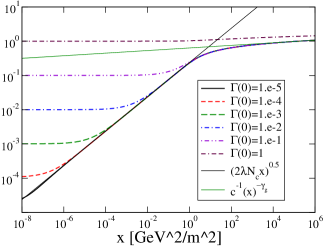
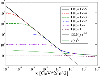
Figure 2: Results for the ghost dressing functions $\Gamma(x)$ [left panel] and $D(x)$ [right panel]. See text for details.

In the UV region, all solutions with different $\Gamma(0)<0.1$ tend to the same curve (the case $\Gamma(0)=1$ will be discussed presently). Asymptotically, it is seen that these solutions obey

$$\Gamma(x)^{-1}=D_{\overline{c}c}^{R}(x)=cx^{\gamma_{g}},$$ (4.1)

where $c\approx 1.581$ and confirming that one recovers the (resummed) perturbative behavior for large $x$. That all curves have the same asymptotic large $x$ behavior suggests that for a large renormalization scale $\mu$ (and after scaling variables with $m^{2}$, $\mu$ would have to be asymptotically large), there is a unique value of $\Gamma(\mu)$ (or vanishingly small differences between different values) for arbitrary input $\Gamma(0)$. We can thus infer that our input $\Gamma(0)$ (at least for moderate values) has nothing to do with the perturbative regime and its renormalization – it is genuinely nonperturbative in origin.

Continuing with the UV region, results for $Z_{c}$ are given in Table 1. Effectively, $Z_{c}\sim 1$ and for the $\Lambda$ and $\Gamma(0)$ values sampled is slowly varying, increasing with $\Lambda$ like $Z_{c}(\Lambda)\sim\ln{\Lambda}$ as one would have expected from the perturbative result (and with fixed spatial gluon input and a tree-level vertex, this is not surprising). Noticing the behavior of $Z_{c}$ for different values of input $\Gamma(0)$, we plot $Z_{c}$ as a function of $\Gamma(0)$ for fixed $\Lambda=10^{6}[\mbox{GeV}]^{2}/m^{2}$ in Fig. 3. It is seen that $Z_{c}$ is roughly constant for input values less than $\Gamma(0)\sim 0.3$ and this gives an estimate of the largest value of $\Gamma(0)$ for which the ghost solution does not change in the UV. This maximum value of $\Gamma(0)$ loosely corresponds to the situation where the solution curve $\Gamma(x)$ loses contact with the common (asymptotic) large $x$ curve in Fig. 2 (as illustrated for the case $\Gamma(0)=1$). The inference is that there is a region of values $0\leq\Gamma(0)<0.3$ for which the input constant $\Gamma(0)$ is unimportant to the UV. We shall discuss this later in more detail.

$\Gamma(0)$	$1$	$1$	$10^{-2}$	$10^{-2}$	$10^{-4}$	$10^{-4}$	$0$	$0$	$0$	$0$
$\Lambda$	$10^{6}$	$10^{8}$	$10^{6}$	$10^{8}$	$10^{6}$	$10^{8}$	$10^{6}$	$10^{7}$	$10^{8}$	$10^{9}$
$Z_{c}$	$1.45$	$1.57$	$1.09$	$1.24$	$1.09$	$1.24$	$1.09$	$1.17$	$1.24$	$1.31$

Table 1: Numerical results for the renormalization coefficient $Z_{c}$. Dimensionful quantities are in units of $[\mbox{GeV}]^{2}/m^{2}$, see text for details.

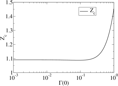
Figure 3: Plot of the ghost renormalization coefficient $Z_{c}$ as a function of $\Gamma(0)$. See text for details.

Returning to Fig. 2, in the infrared region for small $\Gamma(0)$ ($<0.1$) the solution has a region for which the naive powerlaw solution holds and as $\Gamma(0)$ is decreased, one can see that this region extends further into the infrared. Moreover, extrapolating to the case $\Gamma(0)=0$ by eye, one can see that the pure powerlaw solution does exist. Let us emphasize that the powerlaw has not been artificially introduced into the numerical solution via sophisticated techniques (and for which the numerical stability could be improved to an arbitrary degree). The results are obtained using iteration and a direct numerical integration grid: the observed infrared behavior is an independent result. The ‘fitted’ (i.e., fitted by eye) form of the powerlaw solution has one input parameter - the coefficient (the exponent was fixed from the earlier analysis). Clearly, the coefficient must have the factor $\sqrt{\lambda N_{c}}$ but that the factor $\sqrt{2}$ works so well is not explained (and given the previous discussions about the normalization of $D_{AA}^{T}$ is not really relevant). To summarize the IR behavior: the most notable feature of the various solutions is that when going from the common UV asymptotic solution towards small $x$, for a given input boundary condition $\Gamma(0)$ the system has a ‘preferred’ dynamical curve corresponding to the powerlaw case $\Gamma(0)=0$ until ‘forced’ to deviate to the constant boundary value (if $\Gamma(0)\neq 0$).

In the case of the pure powerlaw solution (numerically here, the lowest value of $\Gamma(0)=10^{-5}$), we find that the ghost propagator dressing function solution can be well reproduced over the entire momentum range by the form

$$D_{\overline{c}c}(x)=\frac{1}{\sqrt{2\lambda N_{c}}}\sqrt{\frac{(1-a)}{x}+\frac{a}{\ln{(1+x)}}},$$ (4.2)

with a single parameter, $a\approx 0.689$ (we find that $a$ is slightly dependent on $\Lambda$, which has here the value $\Lambda=10^{6}$ in the scaled units). The comparison is shown in Fig. 4. One can see that the form given in Eq. (4.2) will exactly reproduce the known infrared behavior because of the small $x$ expansion of the logarithm. That the large momentum behavior is, up to a constant, given by $1/\sqrt{\ln{x}}$ was also found in Ref. Feuchter:2004mk . Recall that it was earlier seen that the propagator dressing function behaves as $\sim x^{\gamma_{g}}$ for asymptotically large $x$: the $1/\sqrt{\ln{x}}$ behavior represents an alternative description to the naive perturbative anomalous dimension and indeed appears superior since it is valid over a wide range of momenta.

Figure 4: Plot of the ghost propagator dressing function in the case $\Gamma(0)=10^{-5}$ (indistinguishable from the powerlaw for the scales shown) compared with the fit formula Eq. (4.2). See text for details.

IV.1 Comparison with lattice results

We have seen that using a lattice inspired result Burgio:2008jr as input for the spatial gluon propagator, the ghost propagator dressing function either has an infrared divergence characterized by the exponent $1/2$, or is constant in the infrared depending on the boundary condition $\Gamma(0)$. This result could be compared to the corresponding lattice results. Various studies Cucchieri:2000gu ; Langfeld:2004qs ; Nakagawa:2009zf ; Quandt:2008zj have reported an infrared divergence, i.e., a propagator dressing function of the form $x^{-\kappa}$ for small $x$, but with an exponent $\kappa\approx 0.2-0.25$ (all studies agree on the Gribov form for the equaltime spatial gluon propagator), apparently in contradiction to the results here and from the canonical approach Feuchter:2004mk ; Schleifenbaum:2006bq (where $\kappa=1/2$).

The aforementioned lattice studies naturally involve a smallest infrared spatial momentum scale $\vec{k}^{2}/m^{2}=x_{min}$ and $x_{min}\approx 0.25-0.5$. To extract the infrared exponent $\kappa$, one requires a range of momenta for which the powerlaw relationship holds (or the constant $\Gamma(0)$ is clearly visible). However, taking this range to be, for example, one order of magnitude (i.e., $x=[0.25,2.5]$) and comparing with the results displayed in Fig. 2, one sees that all curves (with $0\leq\Gamma(0)<0.3$) are still within the transition region where the exponent changes from the perturbative value ($x^{\gamma_{g}}$) to the infrared ($x^{-1/2}$). In other words, it may be that the lattice results have not yet genuinely probed far enough into the infrared to see the full exponent.

There is however the possibility that the lattice results might be infrared constant. In Fig. 5, as an illustrative example, we compare the results for the infrared divergent ghost propagator dressing function (numerical and infrared powerlaw, corresponding to $\kappa=0.5$) with the numerical curve for $\Gamma(0)=0.2$ and a fit form with $\kappa=0.2$. Also shown is the perturbative asymptotic result. Importantly, for a wide range of values ($x\approx[0.25,10]$) the curves with $\Gamma(0)=0.2$ and $\kappa=0.2$ are indistinguishable. Whilst this is only an illustration, it does give an alternative explanation to the lower lattice value of $\kappa$ as corresponding to a nonzero value of $\Gamma(0)$ whilst not contradicting the earlier infrared analysis. Again, the deciding factor is that $x_{min}$ cannot be arbitrarily lowered. Note also that since the lattice results with $x_{min}\sim 0.25$ do see an infrared enhancement with $\kappa=0.2$ rather than a constant behavior for the dressing function, this would presumably place an upper bound on the value of the boundary condition: roughly $\Gamma(0)\leq 0.2$.

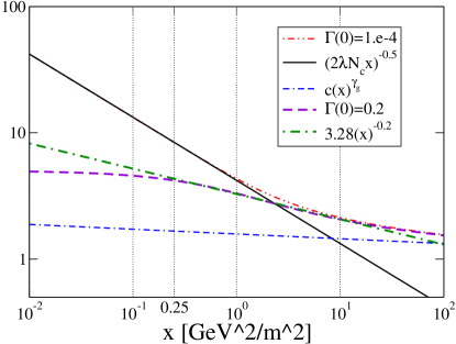
Figure 5: Plot of the ghost propagator dressing function in the case $\Gamma(0)=10^{-4}$ (indistinguishable from $\Gamma(0)=0$ on the scales shown) and $\Gamma(0)=0.2$ compared with the powerlaws characterized by the exponents $\kappa=-\gamma_{g}$ (perturbative), $\kappa=0.2$ (illustrative lattice result) and $\kappa=1/2$ (infrared analysis). The scale $x=0.25$ roughly corresponds to the lowest lattice momenta. See text for details.

To summarize, it would appear that in order to discriminate between the various infrared solutions, the lattice studies have not yet gone far enough into the infrared to give a clear signal that one has a particular value of the exponent $\kappa$, or a particular boundary condition $\Gamma(0)$. Such studies are planned mqgb and using the analysis of the ghost Dyson-Schwinger equation presented in this study may be of help in the extraction of the infrared behavior.

V Discussion of the results

In this Section, we shall present and discuss arguments for the possible interpretation of the numerical results. To this purpose, we shall draw on various different ideas and concepts. In order to aid clarity, we split the discussion into different parts. The first part reiterates the identification of $\Gamma(0)$ as a boundary condition. The second then addresses the issue of the physical interpretation of such a boundary condition and its connection to the Gribov gauge fixing ambiguity. The third part then continues by turning the arguments round, resulting in a conjecture that physical results may actually be independent of the value of the boundary conditions. The final part then discusses an alternate interpretation of $\Gamma(0)$ as being concerned with the renormalization scheme and why this is seemingly ruled out by the results here.

V.0.1 $\Gamma(0)$ as a boundary condition.

That the various infrared solutions of the ghost Dyson-Schwinger equation are delineated by some constant, $\Gamma(0)$, should not come as a surprise. Indeed, this has been explicitly seen in the canonical approach to Coulomb gauge Epple:2007ut and there is a similar situation in Landau gauge as discussed in the Introduction. The Dyson-Schwinger equations are derived as functional differential equations that can only relate Green’s functions and as such, require (functional) boundary conditions to finally specify a value for a given Green’s function. Clearly the solutions should agree with the asymptotic perturbative expansion in the vicinity of the renormalization point and the functions should be smooth and continuous for finite, non-zero momenta (a feature naturally present for an iterative numerical solution). The remaining boundary condition in the case of the ghost Dyson-Schwinger equation is then the value of $\Gamma(0)$. Normally, one would be considering a coupled system of Dyson-Schwinger equations whereby the solution for the gluon propagator is also being sought and the issue of the existence of the boundary condition is invariably obscured by technical details (such as the truncation scheme); here we have utilized the general consensus about the Gribov form for the equaltime spatial gluon propagator to fix this sector so that the existence of the boundary condition as input to choosing the relevant solution is made explicit. Indeed, this is particularly relevant in Coulomb gauge within the functional integral formalism, where the energy divergence of the ghost-loop and the necessary nonperturbative cancellation prohibits a direct back-coupling of the ghost to the gluon polarization.

V.0.2 $\Gamma(0)$ and the Gribov problem.

Having established the requirement for a boundary condition, the important question is thus: is there a particular physical value? To answer this question we obviously need to know to what physics the different solutions correspond to. The most pertinent aspect of the numerical results presented here is that for a wide range of values ($0\leq\Gamma(0)<0.3$), the UV solution and the ghost renormalization coefficient are unaltered and meaning that the boundary condition has nothing to do with either the perturbative region or the renormalization condition (at least conventionally where the renormalization scale is chosen to be perturbative). We can thus conclude that the boundary condition, at least for the ghost Dyson-Schwinger equation in isolation, is connected only to the nonperturbative (infrared) physics. Additionally, that the various solutions exhibit a particular infrared behavior where as one goes from large to small momenta, the curves follow the dynamical solution until ‘forced’ to deviate to the constant boundary value suggests that the boundary condition is connected to a freezing of the dynamics below a particular scale.

Let us now introduce some aspects of Coulomb gauge and the Gribov problem relevant to the discussion here. In the functional approach to Coulomb gauge (within the first order formalism, but the same applies here), the system can be shown to reduce to the ‘would-be-physical’ degrees of freedom Zwanziger:1998ez ; Watson:2006yq ; Reinhardt:2008pr : that is, after resolving Gauss’ law only two transverse spatial gluon degrees of freedom remain (in quantum electrodynamics these would be the physical photon polarization states) and the longitudinal, temporal, and ghost degrees of freedom cancel. In the Gribov-Zwanziger confinement picture Gribov:1977wm ; Zwanziger:1998ez ; Zwanziger:1995cv , the transverse spatial propagator (given by the Gribov formula here) is infrared suppressed and subsequently drops out of the physical spectrum. The reduction to transverse spatial degrees of freedom has the Faddeev-Popov (FP) operator as a central element and the ghost propagator is precisely the expectation value of the inverse of this operator. However, the known existence of zero modes of the FP operator and the associated Gribov ambiguities complicate matters Gribov:1977wm . The Gribov problem is a result of the fact that the gauge is not completely specified. The lack of complete gauge fixing manifests itself in gauge-variant quantities (i.e., the propagators) and implies an ambiguity in the definition of the underlying functional integral. Given that the spatial gluon propagator in Coulomb gauge corresponds to the ‘would-be-physical’ degrees of freedom (in the above sense), one might expect that the Gribov problem would be relatively unimportant – we have, after all, the Gribov form as input; on the other hand, the ghost propagator would be entirely dependent on the resolution of the incomplete gauge-fixing (explicitly found to be the case in 1+1 dimensions Reinhardt:2008ij ). This scenario is the case here with a fixed spatial gluon propagator (the Gribov form) and a ghost that must be specified with further input but that does not directly back-couple to the gluon.

The first part of the argument for a connection between the Gribov problem and the boundary condition $\Gamma(0)$ goes as follows. In the presence of the Gribov ambiguity, the form of the Dyson-Schwinger equations (at least in more than one spatial dimension for Coulomb gauge) is unchanged Zwanziger:2003cf . The implication is that the dynamical behavior of the solutions would not be affected by the existence of Gribov copies and this is consistent with the characteristic pattern of the results here (Fig. 2) where with various values of $\Gamma(0)$ (at least for the range $0\leq\Gamma(0)<0.3$) as $\Gamma(0)$ is lowered, the solutions follow the same dynamical curve further into the infrared before freezing out to the value $\Gamma(0)$ imposed as the boundary condition.

The second part of the argument connecting $\Gamma(0)$ and the Gribov ambiguity concerns the following observation. Generally, when (improperly) integrating over the gauge group, gauge-dependent functional integrals (propagators) would be suppressed by averaging over the gauge copies. This is an important point: gauge copies either have the same phase in group space when contributing to the functional integral in which case the integration over the gauge copies is merely an unobservable constant in the normalization; or if the gauge copies have a different phase then the integration over the group space can only reduce a gauge-dependent functional integral. Gribov copies are accompanied by zero modes of the Faddeev-Popov operator, which for Coulomb gauge reads

$$-{\vec{\nabla}}\!\cdot\!{\vec{D}^{ab}[\vec{A}]},\;\;\;\;\vec{D}^{ab}[\vec{A}]=\delta^{ab}\vec{\nabla}-gf^{acb}\vec{A}^{c}(x).$$ (5.1)

Perturbatively, in the sense of an expansion in the gauge field ($\vec{A}$) around zero there are no Gribov copies such that the perturbative regime would be insensitive. The ghost propagator results are insensitive to $\Gamma(0)$ at large momenta where perturbation theory is valid (as explicitly demonstrated previously). In the nonperturbative case, for low momenta, there are ‘more’ Gribov copies (we do not know how to count the number, but from the form of the Faddeev-Popov operator, the large fields $\vec{A}$ within the covariant derivative that account for the existence of Gribov copies are large in the sense of their relationship to the spatial differential operator, which in momentum space translates, loosely speaking, to the spatial momentum). There are two plausible signals for the possible presence of Gribov copies within the functional integral for the ghost propagator arising from improper gauge averaging: 1) below a certain momentum scale, the averaging over the gauge group induced by the existence of Gribov copies might serve to freeze the functional integral to a specific value and 2) for successively lower momenta, the difference between a functional integral affected by Gribov copies and one that isn’t would increase. The results in this study show that for finite $\Gamma(0)$, there is precisely such a freezing below a particular scale whereas for $\Gamma(0)=0$ there isn’t. Also, the difference between the various solutions with finite and zero values of $\Gamma(0)$ does increase with successively lower momenta. Now, $\Gamma(0)$ is a boundary condition specifying a particular allowed solution of the Dyson-Schwinger equation and thereby implicitly selecting a definition of the ghost propagator functional integral from the various possibilities given that there is an ambiguity in the gauge fixing. That for different values of $\Gamma(0)$, the results explicitly exhibit the characteristics that one would expect in the possible presence of Gribov copies suggests that $\Gamma(0)$ is indeed intimately connected to the Gribov problem. The case $\Gamma(0)=0$ would appear to correspond to that implicit definition of the functional integral for the ghost where the Gribov copies have no effect, i.e., the curve is purely dynamical and there is no freezing in the infrared. For finite $\Gamma(0)$, the dynamical curve freezes below a certain scale indicating the influence of Gribov copies and their averaging.

There are two further arguments connecting $\Gamma(0)$ and the Gribov problem that are known in Coulomb gauge: Gribov’s original work Gribov:1977wm and the case of $1+1$-dimensions Reinhardt:2008ij . In Ref. Gribov:1977wm , the perturbative aspects of the ghost propagator were discussed. In the language used here, in order to ensure the absence of gauge copies (in the sense that the FP operator be positive definite), the restriction $\Gamma(0)\geq 0$ was introduced. In the case of $1+1$-dimensional Coulomb gauge (where because the ‘physical’ transverse spatial propagator cannot exist, the system reduces to purely a discussion of the gauge-fixing and Gribov copies) it was seen explicitly that the ghost propagator functional integral after resolving the Gribov problem was that with effectively the lowest allowed positive value of the boundary condition (due to the spatial compactification of the underlying manifold employed there, one could not assign a value of $\Gamma(x)$ for $x=0$). Functional integrals constructed to include Gribov copies had different boundary conditions, but obeyed the same Dyson-Schwinger equation.

One objection to the above assertion that $\Gamma(0)=0$ corresponds to the situation where Gribov copies have no effect is of course that the lattice data may be consistent with the solution for $\Gamma(0)\sim 0.2$ as discussed earlier. That the ghost dressing function is infrared finite seems to be the case in Landau gauge on the lattice (see for example Ref. Cucchieri:2010xr and references therein). However, it could be that the different results are not in conflict but are results for different problems. Gribov copies are the consequence of an incomplete gauge fixing, which manifests itself in the eigenspectrum of the Faddeev-Popov operator and this eigenspectrum is obviously dependent on the boundary conditions one assigns to the eigenfunctions. Namely, the Gribov problem may be different for a compact manifold (the lattice with periodic boundary conditions) or in the continuum (with a flat Minkowski/Euclidean metric and boundary conditions at infinity) and also different when comparing Coulomb and Landau gauges Greensite:2010hn . When inserted into the functional integral, it is then currently an open question as to what effect this might have.

V.0.3 $\Gamma(0)$ as an implicit gauge choice.

Another way to view the connection between $\Gamma(0)$ and the Gribov problem is that it can be conjectured that the additional (nonlocal) gauge fixing required to eliminate Gribov copies is linked to the discussion of a specific choice for $\Gamma(0)$. However, turning the argument around, one could interpret $\Gamma(0)$ as a choice of gauge, as was proposed in Ref. Maas:2009se . More properly, the interpretation of $\Gamma(0)$ would be as a choice of gauge completion: the overall gauge choice (Landau or Coulomb gauge, for example) is required to have a well-defined perturbative propagator and because the dynamical solution to the Dyson-Schwinger equation must be smoothly and continuously connected to this perturbative expression in the ultraviolet, then the lack of complete gauge fixing does not mean that the Green’s function is ill-defined, rather that there exist multiple solutions and the choice of gauge completion defines the nonperturbative component of the propagator in the sense that a specific solution (corresponding to a particular value of the boundary condition) is chosen. Indeed, the interpretation of the boundary condition $\Gamma(0)$ as an implicit choice of gauge is rather convenient since as long as one can show that the different choices are physically equivalent, one can choose the gauge so as to make specific calculations more straightforward. That is to say that whilst the elimination of Gribov copies may indeed provide a definite value for $\Gamma(0)$, the arbitrariness is to do with the gauge fixing and one may specify any gauge one desires. This provides a possible answer to the original question about the existence of a particular physical value for the boundary condition $\Gamma(0)$ – there may be no unique physical value, just as propagators are different in different gauges. Furthermore, issues such as the confinement mechanism may appear different for different choices of $\Gamma(0)$. The task would of course be to eventually show that the same physical results can be obtained with different boundary conditions. We shall briefly discuss the case $\Gamma(0)=0$ below.

V.0.4 $\Gamma(0)$ as a renormalization scheme.

As a final remark here, another interpretation of the boundary condition is that the value of $\Gamma(0)$ is a choice of the renormalization scheme to absorb constants into the renormalization coefficient $Z_{c}$, and which again is a free choice (and which has no impact on the perturbative renormalization). The Gribov-Zwanziger confinement scenario Gribov:1977wm ; Zwanziger:1998ez ; Zwanziger:1995cv motivates the choice $\Gamma(0)=0$. However, that the renormalization coefficient $Z_{c}$ is seen to be stable for a range of values, $\Gamma(0)$ (see Fig. 3), would seem to rule out this interpretation of $Z_{c}$ for this aspect of the Gribov-Zwanziger scenario in Coulomb gauge.

VI Critical ghost confinement and infrared slavery

As has been seen, when the boundary condition $\Gamma(0)=0$, the ghost propagator dressing function behaves like $1/|\vec{k}|$ in the infrared. This is of course the result for the so-called critical solutions obtained in the canonical formalism and provides a very simple picture for many aspects of confinement Reinhardt:2008ek ; Reinhardt:2009ks . In the functional formalism, the infrared critical (powerlaw) ghost solution provides an important possible addition to this list, as we shall now motivate.

The ghost and spatial gluon propagators have been discussed so far, but in the functional approach to Coulomb gauge there is a third propagator – the temporal gluon propagator corresponding to the temporal component of the gluon field ($\sigma\equiv A^{0}$). In the canonical approach to Coulomb gauge, one starts with Weyl gauge ($\sigma=0$) and then imposes Coulomb gauge Christ:1980ku ; Feuchter:2004mk , so the temporal gluon propagator does not exist in this sense (the analogous quantity to the temporal gluon propagator in the canonical formalism is the non-Abelian color potential). Within the functional formalism in the heavy quark limit, it has been shown that when the temporal gluon propagator diverges like $1/\vec{k}^{4}$ (or equivalently, that the dressing function goes like $1/\vec{k}^{2}$) in the infrared, one directly obtains a linear rising potential (and bound states) for color singlet quark-antiquark and diquark (for $N_{c}=2$ colors) configurations with no finite energy colored states permitted and corresponding precisely to the old infrared slavery picture of confinement Popovici:2010mb . The lattice results for the temporal gluon propagator do exhibit this infrared behavior Quandt:2008zj ; Cucchieri:2000gu .

The decomposition of the temporal gluon propagator and proper two-point function reads Watson:2007vc :

$$W_{\sigma\sigma}^{ab}(k)=\imath\delta^{ab}\frac{D_{\sigma\sigma}(k_{0}^{2},\vec{k}^{2})}{\vec{k}^{2}},\;\;\;\;\Gamma_{\sigma\sigma}^{ab}(k)=-\imath\delta^{ab}\vec{k}^{2}\Gamma_{\sigma\sigma}(k_{0}^{2},\vec{k}^{2}),\;\;\;\;D_{\sigma\sigma}(k_{0}^{2},\vec{k}^{2})\Gamma_{\sigma\sigma}(k_{0}^{2},\vec{k}^{2})=1.$$ (6.1)

In addition, the decomposition of the proper spatial gluon two-point function (the spatial gluon polarization) is

$$\Gamma_{AAij}^{ab}(k)=-\imath\delta^{ab}\left[k^{2}t_{ij}(\vec{k})\Gamma_{AA}(k_{0}^{2},\vec{k}^{2})+k_{0}^{2}\frac{k_{i}k_{j}}{\vec{k}^{2}}\overline{\Gamma}_{AA}(k_{0}^{2},\vec{k}^{2})\right],$$ (6.2)

where the dressing function $\Gamma_{AA}$ is the inverse of $D_{AA}$ and $\overline{\Gamma}_{AA}$ is the longitudinal dressing function component of the polarization (in Coulomb gauge, this quantity is emphatically not vanishing unlike in Landau gauge). Importantly, the Slavnov-Taylor identity for the two-point functions tells us that Watson:2008fb

$$\Gamma_{\sigma\sigma}(k_{0}^{2},\vec{k}^{2})=\overline{\Gamma}_{AA}(k_{0}^{2},\vec{k}^{2})\left[\Gamma_{\overline{c}c}(\vec{k}^{2})\right]^{2}$$ (6.3)

(we replace the subscripts for $\Gamma_{\overline{c}c}$ to avoid confusion). On general grounds, it can be shown that $D_{\sigma\sigma}$ (and consequently, $\Gamma_{\sigma\sigma}$) must have a nontrivial instantaneous (energy independent, or $\sim\delta(x_{1}^{0}-x_{2}^{0})$ in configuration space) component Cucchieri:2000hv . In fact, lattice results indicate that there is only a very weak energy dependence for $D_{\sigma\sigma}$ Quandt:2008zj and so it appears that neglecting the non-instantaneous component is a good approximation. In other words

$$D_{\sigma\sigma}(k_{0}^{2},\vec{k}^{2})=D_{\sigma\sigma}(\vec{k}^{2}),\;\;\;\;\Gamma_{\sigma\sigma}(k_{0}^{2},\vec{k}^{2})=\Gamma_{\sigma\sigma}(\vec{k}^{2}),\;\;\;\;\overline{\Gamma}_{AA}(k_{0}^{2},\vec{k}^{2})=\overline{\Gamma}_{AA}(\vec{k}^{2}).$$ (6.4)

Assuming multiplicative renormalizability and assigning the renormalization coefficient $\sqrt{Z_{\sigma}}$ to the temporal gluon field $\sigma$ as before, since both the longitudinal and transverse components of the spatial polarization share the same renormalization coefficient, then we immediately see that

$$Z_{\sigma}=Z_{A}Z_{c}^{2}$$ (6.5)

as a consequence of the Slavnov-Taylor identity, as has been known for some time Zwanziger:1998ez . With Eq. (2.13), the product $g^{2}D_{\sigma\sigma}$ is thus a renormalization group invariant, just as $g^{2}D_{AA}D_{\overline{c}c}^{2}$ is. Taking the infrared powerlaw form for the ghost propagator dressing function (noting the scaling of the variables with $m^{2}$), one infers that

$$g^{2}D_{\sigma\sigma}(\vec{k}^{2})\stackrel{{\scriptstyle\vec{k}^{2}\rightarrow 0}}{{\sim}}\frac{m^{2}}{\vec{k}^{2}\overline{\Gamma}_{AA}(\vec{k}^{2})}$$ (6.6)

meaning that if $\overline{\Gamma}_{AA}$ is a constant in the infrared, one has exactly the temporal gluon interaction required for a linear rising potential in Coulomb gauge. Recall that the lattice results for the spatial gluon propagator indicate that the Gribov scale $m$ is not dependent on the renormalization scale Burgio:2008jr and one had the approximate relationship $m\sim 2\sqrt{\sigma_{w}}$ where $\sigma_{w}$ is the Wilsonian string tension. The numerator factor $m^{2}$ arising from the Gribov formula would be thus entirely consistent with the coefficient of the linear rising potential discussed in Ref. Popovici:2010mb . Also recall that in Coulomb gauge, the spatial gluon propagator corresponds to the ‘would-be-physical’ transverse degrees of freedom which indeed suggests that the Gribov scale should be related to a physically observable scale. So, if $\overline{\Gamma}_{AA}$ were to be a constant in the infrared, there would be a direct connection between the spatial gluon propagator and the confinement potential even though the spatial gluon propagator is infrared vanishing (as suggested by the Gribov-Zwanziger confinement scenario Gribov:1977wm ; Zwanziger:1998ez ; Zwanziger:1995cv ).

That $\overline{\Gamma}_{AA}$ is a constant can be argued by appealing to the dimensional type of infrared analysis employed earlier for the ghost Dyson-Schwinger equation and general arguments for Dyson-Schwinger results seen in Landau gauge. In terms of renormalized quantities and recognizing that the renormalization coefficients are dependent on the regularization scale, $\Lambda$, the ghost Dyson-Schwinger equation reads schematically

$$\Gamma_{\overline{c}c}^{R}(\vec{k}^{2};\mu,\overline{g})=Z_{c}(\mu,\overline{g};\Lambda)+\tilde{Z}_{A}(\mu,\overline{g};\Lambda)\Sigma_{\overline{c}c}(\vec{k}^{2};\mu,\overline{g};\Lambda).$$ (6.7)

Now, with the result that $\tilde{Z}_{A}=1$, the self-energy integral must separate into two components, i.e.,

$$\Sigma_{\overline{c}c}(\vec{k}^{2};\mu,\overline{g};\Lambda)\rightarrow\Sigma_{\overline{c}c}^{fin}(\vec{k}^{2};\mu,\overline{g})+\Sigma_{\overline{c}c}^{div}(\mu,\overline{g};\Lambda)$$ (6.8)

such that the equation can be renormalizable. The earlier dimensional analysis for the infrared could then be performed without reference to the (large) scale $\Lambda$ and $\Sigma_{\overline{c}c}^{div}$ after a straightforward subtraction of the equation for $\vec{k}^{2}=\mu$. Then, counting the powers of $\vec{k}^{2}$ led directly to the powerlaw exponent if one assumed the absence of the infrared constant solution and disregarded the Gribov scale $m$. In the case of the Dyson-Schwinger equation for $\overline{\Gamma}_{AA}$, one has the similar schematic form

$$\overline{\Gamma}_{AA}^{R}(\vec{k}^{2};\mu,\overline{g})=Z_{A}(\mu,\overline{g};\Lambda)+\sum_{i}Z_{i}(\mu,\overline{g};\Lambda)\Sigma_{i}(\vec{k}^{2};\mu,\overline{g};\Lambda)$$ (6.9)

but with many more loop self-energy terms (labeled with the index $i$). The renormalization coefficients $Z_{i}$ are the coefficients for the dressed vertices that enter the corresponding loop integrals and can be explicitly derived from the Slavnov-Taylor identities Watson:2008fb . The important information is that only the spatial ghost-gluon vertex coefficient is trivial ($\tilde{Z}_{A}=1$). Thus, only the ghost loop of the Dyson-Schwinger equation for $\overline{\Gamma}_{AA}$ has a form similar to the ghost self-energy above, as is also the case in Landau gauge. However, in Coulomb gauge this loop is explicitly energy divergent and must cancel. Therefore, one cannot separate the finite ($\Lambda$-independent) and divergent ($\vec{k}^{2}$-independent) parts of any of the loop integrals $\Sigma_{i}$ and the dimensional analysis, which relies on this decomposition, cannot hold. This argument would also be true for the Dyson-Schwinger equations for $\Gamma_{AA}$ (the transverse part of the polarization). Actually, the lack of such a separation between infrared and ultraviolet parts of the self-energy terms is another of the difficult technical problems associated with the functional approach to Coulomb gauge and is an explicit demonstration of the difference to Landau gauge (where it is the ghost loop that is the important infrared contribution to the polarization von Smekal:1997vx ).

In the absence of the dimensional analysis, the infrared character of the Dyson-Schwinger equations cannot be directly inferred. However, one can use the experience gained from Landau gauge to anticipate the likely outcome. It has been known for a long time that in Landau gauge, there exist potential quadratic UV divergences in the tensor component of the polarization that is proportional to the metric, which here would be the transverse part of the spatial gluon polarization (i.e., the Dyson-Schwinger equation for $\Gamma_{AA}$) Brown:1988bn (see also Ref. Fischer:2008uz and references therein). Thus, one would naively expect terms in the unrenormalized equation for the dimensionless dressing function that behave like $\Lambda/\vec{k}^{2}$, but which should cancel with a proper regularization procedure (and ignoring in this case the energy dependence). After regularization and renormalization (which doesn’t alter the $\vec{k}^{2}$-dependence), such terms can only be of the form $m^{2}/\vec{k}^{2}$ or $\mu/\vec{k}^{2}$, with any other terms being infrared subleading. Thus, one would expect an infrared behavior for $D_{AA}=\Gamma_{AA}^{-1}$ of the form

$$D_{AA}\stackrel{{\scriptstyle\vec{k}^{2}\rightarrow 0}}{{\sim}}\vec{k}^{2},$$ (6.10)

which is exactly the case for the Gribov formula (and observed on the lattice). For the longitudinal part of the polarization, one would expect logarithmic UV divergences and in the presence of the additional Gribov scale $m$, this would indeed favor a constant type of infrared solution, just as is the case for the dressing functions in the fermion sector of QCD (see for example Ref. Alkofer:2002bp ):

$$\overline{\Gamma}_{AA}\stackrel{{\scriptstyle\vec{k}^{2}\rightarrow 0}}{{\sim}}\mbox{const}.$$ (6.11)

In other words, one can justify that $\overline{\Gamma}_{AA}$ is indeed constant in the infrared such that with the ghost boundary condition $\Gamma(0)=0$, the temporal propagator would be precisely that required for a linearly rising confinement potential.

Obviously, the discussion of this section is somewhat speculative and is certainly intended more to discuss the plausibility of a simple confinement scenario in Coulomb gauge than as a quantitative calculation. One example of a technical complication that might arise in such a quantitative study is that the Slavnov-Taylor identities are in general deformed by the presence of a UV cutoff scale $\Lambda$: in Landau gauge, this has been explicitly studied in Ref. Fischer:2008uz (and references therein). However, what should be amply clear is that the confinement mechanism in Coulomb gauge is certainly dependent on the ghost boundary condition $\Gamma(0)$, underscoring the necessity of pursuing the understanding of the ghost propagator in the infrared further.

VII Summary and outlook

In this study, the ghost Dyson-Schwinger equation in Coulomb gauge has been considered numerically using lattice input for the spatial gluon propagator. It is demonstrated that the dynamical solution must be explicitly supplemented by a nonperturbative boundary condition (the value of the inverse ghost propagator dressing function at zero spatial momentum). With various values of this boundary condition, the solutions have a characteristic behavior: in the ultraviolet, all solutions lie on top of each other and agree with the asymptotic leading order perturbative result; going from high to low momenta, the solutions follow the common dynamical curve into the infrared until freezing out at a point determined by the boundary condition. In this way, it is seen that both critical (powerlaw) and subcritical (infrared finite) solutions exist. It was seen that the critical solution is characterized in the infrared by the exponent $\alpha=1/2$. The ghost renormalization coefficient was observed to be largely independent of the boundary condition. A qualitative comparison to lattice results for the ghost propagator dressing function was illustrated, with the conclusion that it would be desirable to have lattices that go further into the infrared in order to discriminate between the critical and subcritical solutions. The characteristic pattern of the solutions for different boundary conditions can be naturally interpreted in terms of the Gribov gauge fixing ambiguity and it is conjectured that if the boundary condition is related to a choice of gauge fixing completion, then physical (gauge invariant) results should not be dependent on the choice. Plausibility arguments are put forward that connect the critical solution for the ghost propagator dressing function with the temporal gluon propagator and the confinement mechanism.

Whilst the aim of this study was to demonstrate the explicit requirement for a nonperturbative boundary condition to supplement the dynamical solution of the ghost Dyson-Schwinger equation in Coulomb gauge and to present numerical results, the characteristic behavior that was found led to two primary conjectures. Clearly then, the task will be to investigate further. The first conjecture is that the boundary condition studied here is connected to the resolution of the Gribov problem in Coulomb gauge. Work is currently underway to study this connection explicitly prog . The second conjecture concerns the connection of the ghost propagator to confinement via the temporal and longitudinal spatial gluon proper two-point functions courtesy of the Slavnov-Taylor identities. This is a formidable task because of the inherent technical difficulties of solving the Dyson-Schwinger equations within the noncovariant Coulomb gauge functional formalism; however, these technical problems are being steadily overcome and one may hope for concrete results within a reasonable timeframe.

- (1) S. Mandelstam, Phys. Rev. D 20, 3223 (1979).
- (2) U. Bar-Gadda, Nucl. Phys. B 163, 312 (1980).
- (3) L. von Smekal, A. Hauck and R. Alkofer, Annals Phys. 267, 1 (1998) [Erratum-ibid. 269, 182 (1998)] [arXiv:hep-ph/9707327].
- (4) D. Atkinson and J. C. R. Bloch, Phys. Rev. D 58, 094036 (1998) [arXiv:hep-ph/9712459].
- (5) D. Atkinson and J. C. R. Bloch, Mod. Phys. Lett. A 13, 1055 (1998) [arXiv:hep-ph/9802239].
- (6) P. Watson and R. Alkofer, Phys. Rev. Lett. 86, 5239 (2001) [arXiv:hep-ph/0102332].
- (7) C. Lerche and L. von Smekal, Phys. Rev. D 65, 125006 (2002) [arXiv:hep-ph/0202194].
- (8) R. Alkofer, C. S. Fischer and F. J. Llanes-Estrada, Phys. Lett. B 611, 279 (2005) [Erratum-ibid. 670, 460 (2009)] [arXiv:hep-th/0412330].
- (9) W. Schleifenbaum, A. Maas, J. Wambach and R. Alkofer, Phys. Rev. D 72, 014017 (2005) [arXiv:hep-ph/0411052].
- (10) R. Alkofer and L. von Smekal, Phys. Rept. 353, 281 (2001) [arXiv:hep-ph/0007355].
- (11) C. S. Fischer, J. Phys. G 32, R253 (2006) [arXiv:hep-ph/0605173].
- (12) R. Oehme and W. Zimmermann, Phys. Rev. D 21, 471 (1980).
- (13) T. Kugo and I. Ojima, Prog. Theor. Phys. Suppl. 66, 1 (1979); N. Nakanishi and I. Ojima, World Sci. Lect. Notes Phys. 27, 1 (1990).
- (14) V. N. Gribov, Nucl. Phys. B 139 (1978) 1.
- (15) D. Zwanziger, Nucl. Phys. B 485, 185 (1997) [arXiv:hep-th/9603203].
- (16) D. Zwanziger, Nucl. Phys. B 518 (1998) 237.
- (17) A. Cucchieri and T. Mendes, Phys. Rev. Lett. 100, 241601 (2008) [arXiv:0712.3517 [hep-lat]].
- (18) A. Cucchieri and T. Mendes, Phys. Rev. D 78, 094503 (2008) [arXiv:0804.2371 [hep-lat]].
- (19) A. Cucchieri and T. Mendes, PoS QCD-TNT09, 026 (2009) [arXiv:1001.2584 [hep-lat]].
- (20) P. Boucaud, J. P. Leroy, A. L. Yaouanc, J. Micheli, O. Pene and J. Rodriguez-Quintero, JHEP 0806, 012 (2008) [arXiv:0801.2721 [hep-ph]].
- (21) Ph. Boucaud, J. P. Leroy, A. Le Yaouanc, J. Micheli, O. Pene and J. Rodriguez-Quintero, JHEP 0806, 099 (2008) [arXiv:0803.2161 [hep-ph]].
- (22) C. S. Fischer, A. Maas and J. M. Pawlowski, Annals Phys. 324, 2408 (2009) [arXiv:0810.1987 [hep-ph]].
- (23) A. P. Szczepaniak and E. S. Swanson, Phys. Rev. D 65, 025012 (2002) [arXiv:hep-ph/0107078].
- (24) C. Feuchter and H. Reinhardt, Phys. Rev. D 70 (2004) 105021 [arXiv:hep-th/0408236]; C. Feuchter and H. Reinhardt, arXiv:hep-th/0402106.
- (25) W. Schleifenbaum, M. Leder and H. Reinhardt, Phys. Rev. D 73, 125019 (2006) [arXiv:hep-th/0605115].
- (26) D. Epple, H. Reinhardt and W. Schleifenbaum, Phys. Rev. D 75, 045011 (2007) [arXiv:hep-th/0612241].
- (27) D. Epple, H. Reinhardt, W. Schleifenbaum and A. P. Szczepaniak, Phys. Rev. D 77, 085007 (2008) [arXiv:0712.3694 [hep-th]].
- (28) H. Reinhardt et al., PoS QCD-TNT09, 038 (2009) [arXiv:0911.0613 [hep-th]].
- (29) H. Reinhardt, Phys. Rev. Lett. 101, 061602 (2008) [arXiv:0803.0504 [hep-th]].
- (30) N. H. Christ and T. D. Lee, Phys. Rev. D 22, 939 (1980) [Phys. Scripta 23, 970 (1981)].
- (31) A. Cucchieri and D. Zwanziger, Phys. Rev. D 65, 014001 (2001) [arXiv:hep-lat/0008026].
- (32) K. Langfeld and L. Moyaerts, Phys. Rev. D 70, 074507 (2004) [arXiv:hep-lat/0406024].
- (33) Y. Nakagawa et al., Phys. Rev. D 79, 114504 (2009) [arXiv:0902.4321 [hep-lat]].
- (34) G. Burgio, M. Quandt and H. Reinhardt, Phys. Rev. Lett. 102, 032002 (2009) [arXiv:0807.3291 [hep-lat]].
- (35) M. Quandt, G. Burgio, S. Chimchinda and H. Reinhardt, PoS CONFINEMENT8, 066 (2008) [arXiv:0812.3842 [hep-th]].
- (36) L. Baulieu and D. Zwanziger, Nucl. Phys. B 548, 527 (1999) [arXiv:hep-th/9807024].
- (37) A. Niegawa, M. Inui and H. Kohyama, Phys. Rev. D 74, 105016 (2006) [arXiv:hep-th/0607207].
- (38) D. Zwanziger, Nucl. Phys. B 364, 127 (1991).
- (39) H. Reinhardt and P. Watson, Phys. Rev. D 79, 045013 (2009) [arXiv:0808.2436 [hep-th]].
- (40) P. Watson and H. Reinhardt, Phys. Rev. D 75, 045021 (2007) [arXiv:hep-th/0612114].
- (41) P. Watson and H. Reinhardt, Phys. Rev. D 77, 025030 (2008) [arXiv:0709.3963 [hep-th]].
- (42) C. Popovici, P. Watson and H. Reinhardt, Phys. Rev. D 79, 045006 (2009) [arXiv:0810.4887 [hep-th]].
- (43) P. Watson and H. Reinhardt, Eur. Phys. J. C 65, 567 (2010) [arXiv:0812.1989 [hep-th]].
- (44) C. Popovici, P. Watson and H. Reinhardt, Phys. Rev. D 81, 105011 (2010) [arXiv:1003.3863 [hep-th]].
- (45) P. Watson and H. Reinhardt, Phys. Rev. D 76, 125016 (2007) [arXiv:0709.0140 [hep-th]].
- (46) W. J. Marciano and H. Pagels, Phys. Rept. 36, 137 (1978).
- (47) D. R. Campagnari, H. Reinhardt and A. Weber, Phys. Rev. D 80, 025005 (2009) [arXiv:0904.3490 [hep-th]].
- (48) A. Cucchieri and D. Zwanziger, Phys. Rev. D 65, 014002 (2001) [arXiv:hep-th/0008248].
- (49) M. Quandt and G. Burgio, private communication.
- (50) H. Reinhardt and W. Schleifenbaum, Annals Phys. 324, 735 (2009) [arXiv:0809.1764 [hep-th]].
- (51) D. Zwanziger, Phys. Rev. D 69, 016002 (2004) [arXiv:hep-ph/0303028].
- (52) J. Greensite, Phys. Rev. D 81, 114011 (2010) [arXiv:1001.0784 [hep-th]].
- (53) A. Maas, Phys. Lett. B 689, 107 (2010) [arXiv:0907.5185 [hep-lat]].
- (54) N. Brown and M. R. Pennington, Phys. Rev. D 39, 2723 (1989).
- (55) R. Alkofer, P. Watson and H. Weigel, Phys. Rev. D 65, 094026 (2002) [arXiv:hep-ph/0202053].
- (56) P. Watson, and H. Reinhardt, work in progress.