Perturbations in Matter Bounce with Non-minimal Coupling

Abstract

In this paper, we investigate the perturbations in matter bounce induced from Lee-Wick lagrangian with the involvement of non-minimal coupling to the Einstein Gravity. We find that this extra non-minimal coupling term can cause a red-tilt on the primordial metric perturbation at extremely large scales. It can also lead to large enhancement of reheating of the normal field particles compared to the usual minimal coupling models.

I introduction

Non-singular bouncing cosmology [1] has become one of the important alternative scenarios of inflation [2] as a description of the early universe. In terms of a bounce scenario, the universe travels from a contracting phase to an expanding phase through a non-vanishing minimal size, avoiding the singularity problem which plagues the Standard Big Bang theory [3] or inflationary theory [4]. Moreover, a bounce can occur much below the Planck scale, eliminating the “Transplanckian” problem of which the wavelength of the fluctuation mode we see today will be even smaller than Planck scale and thus in “the zone of ignorance” where high energy effects are robust and Einstein equations might be invalid [5]. In bounce models, fluctuations were generated in contracting phase and transferred into expanding phase through bouncing point, which can give rise to a scale invariant power spectrum as expected by the current observational data [6]. In order to connect the perturbations in contracting phase and expanding phase at the crossing point, the joint condition of Hwang-Vishniac [7] (Deruelle-Mukhanov [8]) can be applied. Besides, bouncing scenario can also be originated from non-relativistic gravity theories [9] and give rise to gravitational waves with running signature and large non-Gaussianities [10].

In the previous studies, a kind of “matter bounce” has been proposed where before and after the bounce, the universe could behave as non-relativistic matter. This scenario can be realized by a kind of “Lee-Wick” (LW) Lagrangian which contains higher derivatives of the field, or equivalently by two scalar fields with an opposite sign of potential. This scenario can give rise to scale invariant power spectrum at large scales, which is consistent with the data [11]. However, one may expect that there are some non-minimal couplings of the matter in the universe to Einstein Gravity in the early universe . In fact, it is argued that the existence of the non-minimal coupling term is required by the quantum corrections and renormalization [12] in quantum gravity in curved space-time. This effect may, by means of modifying Einstein equations, alter the previous result and leave some signals on the power spectrum that can be detected by observations such as CMB analysis. The non-minimal coupling can also be reduced from higher dimensional theories such as brane theory and can get rid of the Big Bang Singularity, which lead to a bouncing universe [18], or lead to the cosmic acceleration, which can be utilized as inflaton in the early time [19] and dark energy at current epoch [20].

This paper aims at investigating the perturbations in the matter bounce model involving the non-minimal coupling. The paper is organized as follows: we first review the model of matter bounce in Sec. II. After that, in Sec. III we take the non-minimal coupling term into account. We investigate the perturbation through the process in detail, and show the solutions for each stage. We also analyze the particle production due to the resonance. All the analytical calculations are done with help of numerical computations. Finally Sec. IV contains conclusions and discussions.

II review of the matter bounce model

In this section, we will start with the matter bounce model carried out in [11]. This model consists of a single scalar field with a high derivative term of a minus sign. Due to this term, the equation of state (EoS) $w$ is possible to go down below $-1$ and violates the null energy condition, which behaves as a “Quintom” matter [21] and makes it possible to realize a bounce. It is useful to have such a term added in the lagrangian. For example, in the well known Lee-Wick theory which was constructed by T.D. Lee and G. C. Wick [22] (see also [23] for the extensive “Lee-Wick standard model” ), the higher derivative term is used to cancel the quadratic divergence of the Higgs mass and thus address the “hierarchy problem”. It is also possible to construct an ultraviolet complete theory which preserves Lorentz invariance and unitarity in terms of Lee-Wick theory [24].

We begin with the Lagrangian in our model to be in the form:

$${\cal L}=\frac{1}{2}\partial_{\mu}\hat{\phi}\partial^{\mu}\hat{\phi}-\frac{1}{2M^{2}}(\partial^{2}\hat{\phi})^{2}-\frac{1}{2}m^{2}\hat{\phi}^{2}-V(\hat{\phi})~{},$$ (1)

where $m$ is the mass of the scalar field $\hat{\phi}$ and $V(\hat{\phi})$ is the potential. A higher derivative term with minus sign is introduced with some new mass scale $M$. For the Higgs sector of Lee-Wick theory, the hierarchy problem is solved if we require that $M\gg m$. After some field rotations, one can write down the effective Lagrangian:

$${\cal L}=\frac{1}{2}\partial_{\mu}\phi\partial^{\mu}\phi-\frac{1}{2}\partial_{\mu}\tilde{\phi}\partial^{\mu}\tilde{\phi}+\frac{1}{2}M^{2}\tilde{\phi}^{2}-\frac{1}{2}m^{2}\phi^{2}-V(\phi,\tilde{\phi})~{},$$ (2)

where $\tilde{\phi}$ is some auxiliary field and $\phi$ is defined as $\phi\equiv\hat{\phi}+\tilde{\phi}$ . Here the mass matrix of the fields has been diagonalized due to the rotation. Usually there may be some interaction terms between the two fields, or some higher order self-interaction terms like $\phi^{4}$, $\tilde{\phi}^{4}$, $\phi^{2}\tilde{\phi}^{2}$ and so on, but here for simplicity and without losing generality, we will have all of them ignored by setting $V(\phi,\tilde{\phi})=0$. In framework of Friedmann-Robertson-Walker (FRW) metric,

$$ds^{2}=dt^{2}-a(t)^{2}d{\bf x}^{2}~{},$$ (3)

it is easy to get the Friedmann equation as:

$$H^{2}=\frac{\kappa^{2}}{3}\bigl{[}\frac{1}{2}{\dot{\phi}}^{2}-\frac{1}{2}{\dot{\tilde{\phi}}}^{2}+\frac{1}{2}m^{2}\phi^{2}-\frac{1}{2}M^{2}\tilde{\phi}^{2}\bigr{]}~{},$$ (4)

where $\kappa^{2}\equiv 8\pi G$, and the equations of motion of the two fields are

$$\ddot{\phi}+3H\dot{\phi}+m^{2}\phi = 0~{},$$

$$\ddot{\tilde{\phi}}+3H\dot{\tilde{\phi}}+M^{2}\tilde{\phi} = 0~{},$$ (5)

respectively.

Let us now take a close look at how the model works to give rise to a bouncing scenario. The bounce happens by the conditions $H=0$ and $\dot{H}>0$, which requires that the total energy density vanish at some point in the universe evolution. Starting off in the contracting phase, both the two fields $\phi$ and $\tilde{\phi}$ oscillate around the extrema of their potential with a growing amplitude due to the anti-friction of the negative Hubble parameter. Therefore, the energy densities of both fields will grow as $a^{-3}(t)$, which behaves like non-relativistic matter. Note that the energy density of $\tilde{\phi}$ is negative and its growth will cancel that of the total energy density of the universe. At the beginning, we assume that it is subdominant than that of $\phi$, but as $M\gg m$, it will grow faster and eventually catch up, canceling all the positive energy density with its kinetic energy overwhelming that of $\phi$, which makes $\dot{H}>0$ and cause bounce to happen. Thus we can see that before and after the bounce, the universe can be viewed as “matter domination” with the effective equation of state $w=0$, while in the neighborhood of the bounce point, the equation of state goes down to $-\infty$ . It is a good approximation to parameterize $w$ in such a way for the following calculations.

In the following section, we will reinvestigate the scenario by taking into account the coupling of the field to Einstein Gravity. We assume that the normal scalar couples to the curvature through some non-minimal coupling term such as $\frac{1}{2}\xi R\phi^{2}$. We will analyze in detail the evolution of the perturbations in presence of this term, including the metric perturbations as well as the effects on particle production. To support our analytical calculations, we will also perform the numerical investigations.

III adding non-minimal coupling term to the LW bounce

III.1 background

In this section, we investigate the system with the inclusion of the non-minimally coupled term. Generally, we can modify Lagrangian (1) in a very general form such as:

$${\cal L}=\frac{1}{2}\partial_{\mu}\hat{\phi}\partial^{\mu}\hat{\phi}-\frac{1}{2M^{2}}(\partial^{2}\hat{\phi})^{2}-\frac{1}{2}m^{2}\hat{\phi}^{2}-V(\hat{\phi})-f(R)h(\hat{\phi})~{},$$ (6)

where $f(R)$ and $h(\hat{\phi})$ are functions of the Ricci scalar $R$ and scalar field $\hat{\phi}$, respectively. By writing it in terms of $\phi$ and $\tilde{\phi}$ in analogy to (2), we can always have:

$${\cal L}=\frac{1}{2}\partial_{\mu}\phi\partial^{\mu}\phi-\frac{1}{2}\partial_{\mu}\tilde{\phi}\partial^{\mu}\tilde{\phi}+\frac{1}{2}M^{2}\tilde{\phi}^{2}-\frac{1}{2}m^{2}\phi^{2}-V(\phi,\tilde{\phi})-f_{1}(R)h_{1}(\phi)-f_{2}(R)h_{2}(\tilde{\phi})~{},$$ (7)

where $f_{1}(R)$, $f_{2}(R)$, $h_{1}(\phi)$ and $h_{2}(\tilde{\phi})$ are inherited from $f(R)h(\hat{\phi})$ in the original Lagrangian. Usually, these functions are very complicated and difficult to analyze. For the sake of simplicity, we adopt a kind of parametrization form in which the coupling of $\phi$ has a very simple form such as $\frac{1}{2}\xi R\phi^{2}$ with a coefficient $\xi$, while that of $\tilde{\phi}$ vanishes. The parameterized Lagrangian is:

$${\cal S}=\int d^{4}x\sqrt{-g}\bigl{[}\frac{R}{2\kappa^{2}}+\frac{1}{2}\partial_{\mu}\phi\partial^{\mu}\phi-\frac{1}{2}\partial_{\mu}\tilde{\phi}\partial^{\mu}\tilde{\phi}+\frac{1}{2}M^{2}\tilde{\phi}^{2}-\frac{1}{2}m^{2}\phi^{2}-\frac{1}{2}\xi R\phi^{2}\bigr{]}~{}.$$ (8)

From this Lagrangian, we obtain the Einstein Equations as:

$$\frac{1-\kappa^{2}\xi\phi^{2}}{\kappa^{2}}G_{\mu\nu}=g_{\mu\nu}[\frac{1}{2}{\dot{\phi}}^{2}-\frac{1}{2}{\dot{\tilde{\phi}}}^{2}+\frac{1}{2}m^{2}\phi^{2}-\frac{1}{2}M^{2}\tilde{\phi}^{2}\bigr{]}-\nabla_{\mu}\phi\nabla_{\nu}\phi+\nabla_{\mu}\tilde{\phi}\nabla_{\nu}\tilde{\phi}-2\xi g_{\mu\nu}({\dot{\phi}}^{2}+\phi\Box\phi)+2\xi(\nabla_{\mu}\phi\nabla_{\nu}\phi+\phi\nabla_{\mu}\nabla_{\nu}\phi)~{},$$ (9)

and the equations of motion of $\phi$ and $\tilde{\phi}$:

$$\ddot{\phi}+3H\dot{\phi}+m^{2}\phi+\xi R\phi = 0~{},$$

$$\ddot{\tilde{\phi}}+3H\dot{\tilde{\phi}}+M^{2}\tilde{\phi} = 0~{},$$ (10)

respectively. In deriving these equations we have made use of the definition $R\equiv g^{\mu\nu}R_{\mu\nu}=6(\dot{H}+2H^{2})$.

Eq. (9) yields equation for Hubble parameter straightforwardly, which is:

$$H^{2}=\frac{\kappa^{2}}{3(1-\kappa^{2}\xi\phi^{2})}[\frac{1}{2}{\dot{\phi}}^{2}-\frac{1}{2}{\dot{\tilde{\phi}}}^{2}+\frac{1}{2}m^{2}\phi^{2}-\frac{1}{2}M^{2}\tilde{\phi}^{2}+6\xi H\phi\dot{\phi}\bigr{]}~{},$$ (11)

and the Ricci scalar is:

$$R=\frac{\kappa^{2}}{1-\kappa^{2}\xi\phi^{2}(1-6\xi)}\bigl{[}-(1-6\xi){\dot{\phi}}^{2}+2(1-3\xi)m^{2}\phi^{2}+{\dot{\tilde{\phi}}}^{2}-2M^{2}\tilde{\phi}^{2}\bigr{]}~{}.$$ (12)

Generally, the additional term will affect the background evolution by modifying the field equations. This may make the analysis sophisticated and undoable. Moreover, if the modification is too large, the bounce may even be prevented. However, for the case of weak coupling, it is still suitable for us to preserve the bounce and take assumption that the background evolution is hardly affected. Thus it will be safe to use all the results obtained in the above section without losing fidelity.

To be more accurate, we test the background evolution numerically. We choose the parameters and initial conditions to be the same as in [11]. We find that up to $|\xi|\sim 0.05$, the background evolution will not be affected very much and a bounce can still happen. But there may be a little difference, where the universe may enter into a small stage with $w\simeq-1$ before bounce, as have been shown in Fig. 1. This is easy to understand from the field equation. In the additional term, $\xi R$ can be viewed as an effective correction to the original mass squared $m^{2}$. At the initial stage where $R$ is not very large, the correction is negligible, and the field evolves as it does without the additional term. But as the universe evolves like pressureless matter, $R$ will get larger and larger. When the Hubble parameter is about to its maximal value, $H\sim m$, the second scalar $\tilde{\phi}$ will begin to dominate the universe where $\dot{H}$ transfers from negative to positive. At this moment, from the definition of $R$, we can see that it suddenly jumps by the amount of $2|\dot{H}|$. This behavior makes the energy density dominate the universe again for a short while, leading to $w\simeq-1$ in this period. As the energy density of $\tilde{\phi}$ grows up and totally dominates the universe, the equation of state goes down to be below $-1$ and drives the bounce to happen. At the bouncing point where the total energy density of the universe vanishes, one can see from Fig. 1 that the equation of state goes down to negative infinity, and as stated before (in the footnote), it is not a real divergence. After the bounce, the EoS will come up to above $-1$ again as the time reversal of the pre-bounce process.

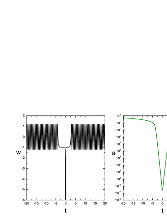
Figure 1: (Color online) Evolution of the background equation of state parameter $w$ and scale factor $a(t)$ in a non-minimal coupling matter bounce model as a function of cosmic time $t$ (horizontal axis). The background fields are plotted in dimensionless units by normalizing by the mass $M_{rec}=10^{-6}m_{pl}$, and the time axis is displayed in units of $M_{rec}^{-1}$. The mass parameters $m$ and $M$ are chosen to be $m=5.0M_{rec}$ and $M=10.0M_{rec}$. The initial conditions are $\phi_{i}=-370.514M_{rec}$, $\dot{\phi}_{i}=-6752.791M_{rec}^{2}$, $\tilde{\phi}_{i}=-4.818\times 10^{-11}M_{rec}$, $\dot{\tilde{\phi}}_{i}=-8.837\times 10^{-11}M_{rec}^{2}$.

III.2 perturbation

In this section we will focus on the perturbation evolution of our model. We begin with the perturbed metric,

$$ds^{2}=a(\eta)^{2}[(1+2\Phi)d\eta^{2}-(1-2\Psi)d{\bf x}^{2}]~{},$$ (13)

in the conformal form. Here $\eta\equiv\int\frac{dt}{a}$ is the conformal time, and $\Phi$ and $\Psi$ are scalar perturbations of the metric. Note that with existence of the non-minimal coupling term, $\Phi$ and $\Psi$ are no longer equivalent. Similarly, the fields can be represented as homogeneous and fluctuation parts as:

$$\phi = \phi_{0}+\delta\phi~{},$$

$$\tilde{\phi} = \tilde{\phi}_{0}+\delta\tilde{\phi}~{}.$$ (14)

In the following, we will neglect the subscript “0” and take $\phi$ and $\tilde{\phi}$ as background components. Then we will solve the perturbed Einstein Equations to see their evolutions.

III.2.1 general solution

From the perturbed Einstein Equation,

$$\delta G_{\mu\nu}=-\kappa^{2}\delta T_{\mu\nu}~{},$$ (15)

we obtain the following equations for perturbation variables:

$$\Phi=\Psi-\frac{\delta F}{F}~{},$$ (16)

$$\dot{\Psi}+(H-\frac{\dot{F}}{2F})\Phi=\frac{\kappa^{2}}{2F}(-\dot{\phi}\delta\phi+\dot{\tilde{\phi}}\delta\tilde{\phi})+\frac{\dot{\delta F}}{2F}+\frac{H\delta F}{2F}~{},$$ (17)

$$\ddot{\Psi}+3(H+\frac{\dot{F}}{2F})\dot{\Psi}+\left\{\frac{\kappa^{2}}{F}\bigl{[}(\dot{\phi}^{2}+12\xi H\phi\dot{\phi})+2\xi\dot{\phi}^{2}\bigr{]}-(2\dot{H}+3H^{2})-\frac{\kappa^{2}m^{2}\phi^{2}}{2F}-\frac{\ddot{F}}{F}\right\}\Psi$$ (18)

$$= \frac{\delta F}{F}\left\{\frac{3}{2}(2\dot{H}+3H^{2})-\frac{\kappa^{2}}{F}\bigl{[}(\frac{\dot{\phi}^{2}}{2}+6\xi H\phi\dot{\phi})+2\xi\dot{\phi}^{2}\bigr{]}+\frac{k^{2}}{2a^{2}}+\frac{\dot{F}^{2}}{2F^{2}}\right\}+\frac{\ddot{\delta F}}{2F}+\frac{\dot{F}\dot{\delta F}}{2F^{2}}$$

$$+ (\frac{\kappa^{2}m^{2}\phi}{F}+\frac{3\kappa^{2}H\dot{\phi}}{F})\delta\phi-\frac{\kappa^{2}}{F}(\frac{\dot{\phi}}{2}+2H\xi\phi)\dot{\delta\phi}~{},$$

$$\ddot{\delta\phi}+3H\dot{\delta\phi}+\left\{\bigl{(}\frac{k}{a}\bigr{)}^{2}+m^{2}+6\xi(\dot{H}+2H^{2})\right\}\delta\phi$$ (19)

$$= 6\xi\phi\ddot{\Psi}+24\xi H\phi\dot{\Psi}+3\dot{\phi}\dot{\Psi}+6\xi H\phi\dot{\Phi}+\dot{\phi}\dot{\Phi}+\frac{4\xi k^{2}\phi\Psi}{a^{2}}+2\xi\phi\bigl{[}6(\dot{H}+2H^{2})-\bigl{(}\frac{k}{a}\bigr{)}^{2}\bigr{]}\Phi-2(m^{2}\phi+\xi R\phi)\Phi~{},$$

where we have defined $F\equiv 1-\kappa^{2}\xi\phi^{2}$.

Since the equations are too sophisticated and there is no hope to solve it directly, we resort to the Einstein frame by a conformal transformation of the metric [27]:

$$\hat{g}_{\mu\nu}=Fg_{\mu\nu}~{}.$$ (20)

The action (8) is then transformed into the form:

$${\cal S}=\int d^{4}x\sqrt{-\hat{g}}\bigl{[}\frac{\hat{R}}{2\kappa^{2}}+\frac{1-(1-6\xi)\kappa^{2}\xi\phi^{2}}{2F^{2}}\hat{\partial}_{\mu}\phi\hat{\partial}^{\mu}\phi-\frac{1}{2F}\hat{\partial}_{\mu}\tilde{\phi}\hat{\partial}^{\mu}\tilde{\phi}+\frac{1}{F^{2}}(\frac{1}{2}M^{2}\tilde{\phi}^{2}-\frac{1}{2}m^{2}\phi^{2})\bigr{]}~{}.$$ (21)

We introduce two new variables, $\chi$ and $\tilde{\chi}$, which are defined as:

$$\chi \equiv \int\frac{\sqrt{1-(1-6\xi)\kappa^{2}\xi\phi^{2}}}{F}d\phi~{},$$

$$\tilde{\chi} \equiv \int\frac{1}{F}d\tilde{\phi}~{},$$ (22)

and rewrite the above action as:

$${\cal S}=\int d^{4}x\sqrt{-\hat{g}}\bigl{[}\frac{\hat{R}}{2\kappa^{2}}+\frac{1}{2}\hat{\partial}_{\mu}\chi\hat{\partial}^{\mu}\chi-\frac{1}{2}\hat{\partial}_{\mu}\tilde{\chi}\hat{\partial}^{\mu}\tilde{\chi}+\frac{1}{F^{2}}(\frac{1}{2}M^{2}\tilde{\phi}(\tilde{\chi})^{2}-\frac{1}{2}m^{2}\phi(\chi)^{2})\bigr{]}~{}.$$ (23)

The perturbed metric will be:

$$ds^{2}=\hat{a}^{2}(\eta)[(1+2\hat{\Phi})d\eta^{2}-(1-2\hat{\Psi})d{\bf x}^{2}]~{},$$ (24)

where $\hat{a}(\eta)=\sqrt{F}a(\eta)$.

For the perturbed metric in Einstein Frame where the off-diagonal components of the perturbed Einstein equations vanishes, we have $\hat{\Phi}=\hat{\Psi}$. This can also be obtained when we consider up to the first order approximation of the perturbed metric, which gives $\hat{\Phi}=\Phi+\frac{\delta F}{2F}$, and $\hat{\Psi}=\Psi-\frac{\delta F}{2F}$ where relation between $\Phi$ and $\Psi$ has already been given in Eq. (16). Moreover, Eq. (17) gives the direct relationship between $\hat{\Phi}$ and the field perturbation,

$$\phi^{\prime}\delta\phi-\tilde{\phi}^{\prime}\delta\tilde{\phi}=\frac{2F^{\frac{3}{2}}(a\sqrt{F}\hat{\Phi})^{\prime}}{\kappa^{2}a[1-(1-6\xi)\kappa^{2}\xi\phi^{2}]}~{},$$ (25)

which is convenient for us to calculate $\hat{\Phi}$ in Einstein frame and then transform into the original Jordan frame.

The equation for $\hat{\Phi}$ is:

$$\hat{\Phi}^{\prime\prime}+2\bigl{(}\hat{\cal H}-\frac{\chi^{\prime\prime}}{\chi^{\prime}}\bigr{)}\hat{\Phi}^{\prime}+2\bigl{(}\hat{\cal H}^{\prime}-\hat{\cal H}\frac{\chi^{\prime\prime}}{\chi^{\prime}}\bigr{)}\hat{\Phi}+k^{2}\hat{\Phi}=\kappa^{2}\bigl{(}2\hat{\cal H}+\frac{\chi^{\prime\prime}}{\chi^{\prime}}\bigr{)}\tilde{\chi}^{\prime}\delta\tilde{\chi}~{},$$ (26)

where $\hat{\cal H}=\hat{a}^{\prime}/\hat{a}$. The right-hand side (r.h.s.) of the equation is assumed to be small and negligible except at the bounce point. Moreover, it is also convenient to define the curvature perturbation $\hat{\zeta}$ in terms of $\hat{\Phi}$:

$$\hat{\zeta}=\hat{\Phi}+\frac{\hat{\cal H}}{\hat{\cal H}^{2}-\hat{\cal H}^{\prime}}(\hat{\Phi}^{\prime}+\hat{\cal H}\hat{\Phi})~{},$$ (27)

which is expected to be conserved on super-Hubble scales in the inflationary universe by the condition that the entropy perturbations are small and $(1+w)\neq 0$:

$$(1+w)\hat{\zeta}^{\prime}=0~{}.$$ (28)

At the next step we will solve Eq. (26) for each stage to get the perturbations $\Phi$, $\Psi$ and $\delta\phi$, and see how it is effected by the non-minimal coupling term.

III.2.2 contracting phase

In contracting phase, the universe is dominated by the normal scalar $\phi$. Since $F$ deos not vary significantly, we roughly have $\tilde{\chi}\sim\tilde{\phi}$ which does not play an important role in the evolution. Then by neglecting the r.h.s. of Eq. (26), we consider it as a homogeneous equation. It is useful to define a new variable $u\equiv\hat{a}\hat{\Phi}/\chi^{\prime}$ and rewrite Eq. (26) as:

$$u^{\prime\prime}+(k^{2}-\frac{\theta^{\prime\prime}}{\theta})u=0~{},$$ (29)

where $\theta=\hat{\cal H}/(\hat{a}\chi^{\prime})$. The solution can be split into two limits: short-wavelength $(k^{2}\gg\theta^{\prime\prime}/\theta)$ and long-wavelength $(k^{2}\ll\theta^{\prime\prime}/\theta)$ where $\theta^{\prime\prime}/\theta$ is the potential. For the short-wavelength perturbations where the potential term can be neglected, we have:

$$u=Ce^{ik\eta}+c.c.~{},$$ (30)

where $C$ is a constant and $c.c.$ stands for the complex conjugate. For long-wavelength perturbations, one gets:

$$u=\theta(S+D\int\frac{d\eta}{\theta^{2}})~{}.$$ (31)

From the above argument of $\Phi$ and $\Psi$ as well as the definition of $u$, one can find the solutions for perturbation variables in terms of $u$ which are:

$$\Phi = \frac{u\hat{\cal H}}{\hat{a}^{2}\theta}-\frac{F^{\prime}}{2\hat{a}F(\hat{\cal H}^{2}-\hat{\cal H}^{\prime})}(\frac{u\hat{\cal H}}{\hat{a}\theta})^{\prime}~{},$$ (32)

$$\Psi = \frac{u\hat{\cal H}}{\hat{a}^{2}\theta}+\frac{F^{\prime}}{2\hat{a}F(\hat{\cal H}^{2}-\hat{\cal H}^{\prime})}(\frac{u\hat{\cal H}}{\hat{a}\theta})^{\prime}~{},$$ (33)

$$\delta\phi = \frac{\phi^{\prime}}{\hat{a}(\hat{\cal H}^{2}-\hat{\cal H}^{\prime})}(\frac{u\hat{\cal H}}{\hat{a}\theta})^{\prime}~{},$$ (34)

where in the last formula we have neglected the contribution arising from $\delta\tilde{\phi}$ in (25), and we have used the approximation $\chi^{\prime 2}\simeq 2(\hat{\cal H}^{2}-\hat{\cal H}^{\prime})/\kappa^{2}$. Substituting (30) or (31) to (32), (33) and (34), we get these variables in Jordan frame:

$$\Phi = C\sqrt{\frac{2}{\kappa^{2}}}\frac{e^{ik\eta}}{\sqrt{-\stackrel{{\scriptstyle\circ}}{{\hat{H}}}}}\left\{-\stackrel{{\scriptstyle\circ}}{{\hat{H}}}-\frac{\stackrel{{\scriptstyle\circ}}{{F}}}{2F}\bigl{(}\hat{H}+\frac{\stackrel{{\scriptstyle\circ\circ}}{{\hat{H}}}}{2\stackrel{{\scriptstyle\circ}}{{\hat{H}}}}+\frac{ik}{\hat{a}}\bigr{)}\right\}+c.c.~{},$$ (35)

$$\Psi = C\sqrt{\frac{2}{\kappa^{2}}}\frac{e^{ik\eta}}{\sqrt{-\stackrel{{\scriptstyle\circ}}{{\hat{H}}}}}\left\{-\stackrel{{\scriptstyle\circ}}{{\hat{H}}}+\frac{\stackrel{{\scriptstyle\circ}}{{F}}}{2F}\bigl{(}\hat{H}+\frac{\stackrel{{\scriptstyle\circ\circ}}{{\hat{H}}}}{2\stackrel{{\scriptstyle\circ}}{{\hat{H}}}}+\frac{ik}{\hat{a}}\bigr{)}\right\}+c.c.~{},$$ (36)

$$\delta\phi = C\stackrel{{\scriptstyle\circ}}{{\phi}}\sqrt{\frac{2}{\kappa^{2}}}\frac{e^{ik\eta}}{\sqrt{-\stackrel{{\scriptstyle\circ}}{{\hat{H}}}}}\bigl{(}\hat{H}+\frac{\stackrel{{\scriptstyle\circ\circ}}{{\hat{H}}}}{2\stackrel{{\scriptstyle\circ}}{{\hat{H}}}}+\frac{ik}{\hat{a}}\bigr{)}+c.c.$$ (37)

for the short-wavelength case, where $\hat{H}$ is the Hubble parameter in Einstein Frame and the symbol $``\circ^{\prime\prime}$ denotes cosmic time derivative in Einstein frame (for details see Appendix A), or

$$\Phi = (\frac{H}{aF}+\frac{\dot{F}}{aF^{2}})S+\frac{2}{\kappa^{2}}D\bigl{[}\frac{1}{F}(\frac{1}{a}\int aFdt)\dot{}-\frac{\dot{F}}{aF^{2}}\int aFdt\bigr{]}~{},$$ (38)

$$\Psi = \frac{H}{aF}S+\frac{2}{\kappa^{2}}D\bigl{[}\frac{1}{F}(\frac{1}{a}\int aFdt)\dot{}\bigr{]}~{},$$ (39)

$$\delta\phi = -\frac{\dot{\phi}}{aF}(S-\frac{2}{\kappa^{2}}D\int aFdt)$$ (40)

for the long-wavelength case. The sketch plot of fluctuation modes compared to $\theta^{\prime\prime}/\theta$ are shown in Fig. 2.

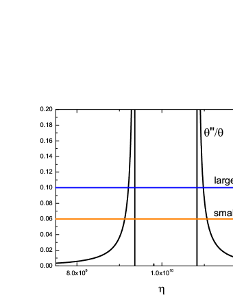
Figure 2: (Color online) A sketch of the evolution of fluctuation modes compared to the potential $\theta^{\prime\prime}/\theta$ in a bouncing universe. The vertical axis is co-moving spatial coordinate, and the horizontal axis is the conformal time. The orange line denotes the fluctuations with small comoving wavenumber $k$ while the blue line is for those with large $k$.

For the case that the universe evolves with some constant equation of state $w$, the scale factor can be parameterized as:

$$a(t)\sim t^{p}~{},$$ (41)

where $p$ is defined as $p\equiv 2/[3(1+w)]$. This will be the case in the whole process except for the bouncing point. During the contracting phase before the non-minimal term dominates the universe, the fields oscillate around their extrema which made the universe behave like non-relativistic matter. The average value of the equation of state of the universe is $<w>=0$ (see from Fig. 1), and the scale factor $a(t)$ scales as $t^{2/3}$. Since in this period the factor $F$ does not evolve significantly, it can be approximately viewed as a constant. Therefore the scaling of $\Phi$, $\Psi$ and $\delta\phi$ are given as:

$$\Phi \simeq \Psi\simeq C\sqrt{\frac{4}{3\kappa^{2}}}\frac{1}{t}e^{-i\frac{k}{a_{0}}t^{\frac{1}{3}}}+c.c.~{},$$ (42)

$$\delta\phi \simeq \frac{2C}{\kappa^{2}\sqrt{F}}(-\frac{1}{3t}+\frac{ik}{a_{0}t^{\frac{2}{3}}})e^{-i\frac{k}{a_{0}}t^{\frac{1}{3}}}+c.c.~{}$$ (43)

for short-wavelength case, and

$$\Phi \simeq \Psi\simeq\frac{2S_{c}^{-}}{3a_{0}Ft^{\frac{5}{3}}}+\frac{6D_{c}^{-}}{5\kappa^{2}}~{},$$ (44)

$$\delta\phi \simeq -\frac{S_{c}^{-}}{a_{0}F}\sqrt{\frac{4}{3\kappa^{2}}}t^{-\frac{5}{3}}+\frac{6D_{c}^{-}}{5\kappa^{2}}\sqrt{\frac{4}{3\kappa^{2}}}~{}$$ (45)

for long-wavelength case, where $a_{0}$ is some normalization constant. Here the subscript $``c"$ denotes the contracting phase and superscript $``-"$ means the matter-like region which happens earlier. Note that $\Phi$, $\Psi$ and $\delta\phi$ have magnitudes of the same order which should be much less than $m_{pl}$, so the difference between $\Phi$ and $\Psi$ (proportional to $\delta\phi$) will be severely suppressed.

However, when the non-minimal term begins to dominate the universe, the equation of state approaches to $-1$. During this period one could define a slow roll parameter $\epsilon\equiv-\dot{H}/H^{2}$ which should be very small. Thus we can have $a=a_{1}t^{1/\epsilon}$ and $H=(\epsilon t)^{-1}$. Moreover, we have from the Einstein Equations that $\dot{\phi}\sim\sqrt{\frac{4}{3\kappa^{2}}}\frac{1}{(t-t_{\ast})}$ and $\phi\sim\sqrt{\frac{4}{3\kappa^{2}}}\ln{(t-t_{\ast})}$, which results in $F=1-\frac{4\xi\phi_{0}}{3}(\ln{(t-t_{\ast})})^{2}$, where $\phi_{0}$ is some constant. From this we can have:

$$\Phi \simeq \Bigl{(}\frac{1}{a_{1}\epsilon(t-t_{\ast})^{1+\frac{1}{\epsilon}}[1-\frac{4\xi\phi_{0}}{3}(\ln{(t-t_{\ast})})^{2}]}-\frac{8\xi\phi_{0}\ln{(t-t_{\ast})}}{3a_{1}(t-t_{\ast})^{1+\frac{1}{\epsilon}}[1-\frac{4\xi\phi_{0}}{3}(\ln{(t-t_{\ast})})^{2}]^{2}}\Bigr{)}S_{c}^{+}$$ (46)

$$+ \frac{2}{\kappa^{2}}\{\epsilon\Bigl{(}\frac{1}{1+\epsilon}+\frac{8\xi\phi_{0}[\epsilon-(1+\epsilon)\ln{(t-t_{\ast})}]}{3(1+\epsilon)^{3}[1-\frac{4\xi\phi_{0}}{3}(\ln{(t-t_{\ast})})^{2}]}\Bigr{)}$$

$$+ \frac{8\epsilon\xi\phi_{0}\ln{(t-t_{\ast})}}{3[1-\frac{4\xi\phi_{0}}{3}(\ln{t})^{2}]}\Bigl{(}\frac{1}{1+\epsilon}-\frac{8\epsilon\xi\phi_{0}[\epsilon+(1+\epsilon)\ln{(t-t_{\ast})}]}{3(1+\epsilon)^{3}[1-\frac{4\xi\phi_{0}}{3}(\ln{(t-t_{\ast})})^{2}]}\Bigr{)}\}D_{c}^{+}~{},$$

$$\Psi \simeq \frac{S_{c}^{+}}{a_{1}\epsilon(t-t_{\ast})^{1+\frac{1}{\epsilon}}[1-\frac{4\xi\phi_{0}}{3}(\ln{(t-t_{\ast})})^{2}]}+\frac{2\epsilon}{\kappa^{2}}\Bigl{(}\frac{1}{1+\epsilon}+\frac{8\xi\phi_{0}[\epsilon-(1+\epsilon)\ln{(t-t_{\ast})}]}{3(1+\epsilon)^{3}[1-\frac{4\xi\phi_{0}}{3}(\ln{(t-t_{\ast})})^{2}]}\Bigr{)}D_{c}^{+}~{},$$ (47)

$$\delta\phi \simeq -\frac{\sqrt{\frac{4}{3\kappa^{2}}}}{a_{1}(t-t_{\ast})^{1+\frac{1}{\epsilon}}[1-\frac{4\xi\phi_{0}}{3}(\ln{(t-t_{\ast})})^{2}]}$$ (48)

$$\left\{S_{c}^{+}-\frac{2a_{1}\epsilon(t-t_{\ast})^{1+\frac{1}{\epsilon}}}{\kappa^{2}(1+\epsilon)^{3}}\Bigl{(}(1+\epsilon)^{2}[1-\frac{4\xi\phi_{0}}{3}(\ln{(t-t_{\ast})})^{2}]-\frac{8\epsilon\xi\phi_{0}}{3}[\epsilon+(1+\epsilon)\ln{(t-t_{\ast})}]\Bigr{)}D_{c}^{+}\right\}~{}$$

for long-wavelength case, where the superscript $``+"$ stands for the deflationary region which comes later.

III.2.3 bouncing phase

When the universe is dominated by the auxiliary scalar $\tilde{\phi}$, the equation of state drops down to below $-1$, and the total energy density of the unverse turns to decrease. When it goes to zero a bounce will happen. It is rather complicated to solve the equation (26) directly, however, we can make some modeling of the evolution to have it simplified without losing fidelity. Generalizing the parametrization method in [11] (see also [28]), we parameterize the Hubble parameter near the bouncing point of the form:

$$H=\alpha_{1}t+\beta_{1}t^{3}+...~{},$$ (49)

with positive constants $\alpha_{1}$ and $\beta_{1}$ of proper dimensions whose magnitudes are determined by the microphysics of the bounce. Note that it is unnecessary to contain terms with even power-laws of $t$. In our case, it can be estimated that $\alpha_{1}\sim m^{2}$. From the relations of variables between Jordan and Einstein frames, we can also obtain the approximate value of $\hat{H}$ with respect to $\hat{t}$ up to first order of $t$:

$$\hat{H}=\alpha\hat{t}+~{}higher~{}order~{}terms~{},$$ (50)

where $\alpha\simeq 4\alpha_{1}/9$. Since this parametrization is only valid during bounce phase where we can neglect the higher order terms of $|\eta-\eta_{B}|$ with $\eta_{B}$ being the comoving time at the bounce point, we obtain the equation for $\hat{\Phi}$ of this phase as:

$$\hat{\Phi}^{\prime\prime}+2y(\eta-\eta_{B})\hat{\Phi}^{\prime}+(k^{2}+\frac{2y}{3})\hat{\Phi}\simeq 0~{},$$ (51)

where $y\equiv 12\alpha a_{B}^{2}/\pi$ and $a_{B}$ is the scale factor at the bounce point. The solution is:

$$\hat{\Phi}=e^{-y(\eta-\eta_{B})^{2}}\left\{EH_{l}(\sqrt{y}(\eta-\eta_{B}))+F_{1}F_{1}\bigl{(}-\frac{l}{2},\frac{1}{2},y(\eta-\eta_{B})^{2}\bigr{)}\right\}~{},$$ (52)

where $H_{l}$ and ${}_{1}F_{1}$ denotes the $l$-th Hermite polynomial and confluent hypergeometric function respectively, with

$$l\equiv-\frac{2}{3}+\frac{k^{2}}{2y}~{}.$$ (53)

The short- and long-wavelength limits of the solution are quite different. For short wavelength $(k^{2}\gg y)$, it reads:

$$\hat{\Phi}=e^{-\frac{y(\eta-\eta_{B})^{2}}{2}}\{\frac{\hat{E}}{\sqrt{2l}}\sin{[k(\eta-\eta_{B})]}+\hat{F}\cos{[k(\eta-\eta_{B})]}\}~{},$$ (54)

while for long wavelength $(k^{2}\ll y)$, it is:

$$\hat{\Phi}=\hat{F}+\hat{E}\sqrt{y}(\eta-\eta_{B})-(1+l)\hat{F}(\eta-\eta_{B})^{2}+{\cal O}((\eta-\eta_{B})^{3})~{},$$ (55)

where $\hat{E}\equiv-2^{1+l}\sqrt{\pi}E/\Gamma(-\frac{l}{2})$ and $\hat{F}\equiv F+2^{l}\sqrt{\pi}E/\Gamma(\frac{1-l}{2})$.

III.2.4 expanding phase

The expanding phase can be viewed as time reversal process of the contracting phase. In this period, both the two fields will roll down along their potentials and begin to oscillate with a decaying amplitude and redshifted energy density. Similar to the case of contracting phase, at the beginning of expansion of the universe, the non-minimal coupling term still remains large and dominate over the mass term of the $\phi$ field, and thus $\phi$ can be approximated as a slow-rolling field. This drives the total equation of state $w$ to approach $-1$, and lead to a short period of inflation. But soon, when the non-minimal coupling term becomes less important, both fields will oscillate around their minimum, behaving like non-relativistic matter again.

One can also get the short and long wavelength solutions of the metric and field perturbations $\Phi$, $\Psi$ and $\delta\phi$ for the expanding phase. We only care about the long-wavelength case which make sense for observation today. As similar to the contracting case just except for replacing the scripts, one gets:

$$\Phi \simeq \Bigl{(}\frac{1}{a_{2}\epsilon(t-t_{{\dagger}})^{1+\frac{1}{\epsilon}}[1-\frac{4\xi\phi_{0}}{3}(\ln{(t-t_{{\dagger}})})^{2}]}-\frac{8\xi\phi_{0}\ln{(t-t_{{\dagger}})}}{3a_{2}(t-t_{{\dagger}})^{1+\frac{1}{\epsilon}}[1-\frac{4\xi\phi_{0}}{3}(\ln{(t-t_{{\dagger}})})^{2}]^{2}}\Bigr{)}S_{e}^{-}$$ (56)

$$+ \frac{2}{\kappa^{2}}\{\epsilon\Bigl{(}\frac{1}{1+\epsilon}+\frac{8\xi\phi_{0}[\epsilon-(1+\epsilon)\ln{(t-t_{{\dagger}})}]}{3(1+\epsilon)^{3}[1-\frac{4\xi\phi_{0}}{3}(\ln{(t-t_{{\dagger}})})^{2}]}\Bigr{)}~{}$$

$$+ \frac{8\epsilon\xi\phi_{0}\ln{(t-t_{{\dagger}})}}{3[1-\frac{4\xi\phi_{0}}{3}(\ln{(t-t_{{\dagger}})})^{2}]}\Bigl{(}\frac{1}{1+\epsilon}-\frac{8\epsilon\xi\phi_{0}[\epsilon+(1+\epsilon)\ln{(t-t_{{\dagger}})}]}{3(1+\epsilon)^{3}[1-\frac{4\xi\phi_{0}}{3}(\ln{(t-t_{{\dagger}})})^{2}]}\Bigr{)}\}D_{e}^{-}~{},$$

$$\Psi \simeq \frac{S_{e}^{-}}{a_{2}\epsilon(t-t_{{\dagger}})^{1+\frac{1}{\epsilon}}[1-\frac{4\xi\phi_{0}}{3}(\ln{(t-t_{{\dagger}})})^{2}]}+\frac{2\epsilon}{\kappa^{2}}\Bigl{(}\frac{1}{1+\epsilon}+\frac{8\xi\phi_{0}[\epsilon-(1+\epsilon)\ln{(t-t_{{\dagger}})}]}{3(1+\epsilon)^{3}[1-\frac{4\xi\phi_{0}}{3}(\ln{(t-t_{{\dagger}})})^{2}]}\Bigr{)}D_{e}^{-}~{},$$ (57)

$$\delta\phi \simeq -\frac{\sqrt{\frac{4}{3\kappa^{2}}}}{a_{2}(t-t_{{\dagger}})^{1+\frac{1}{\epsilon}}[1-\frac{4\xi\phi_{0}}{3}(\ln{(t-t_{{\dagger}})})^{2}]}$$ (58)

$$\left\{S_{e}^{-}-\frac{2a_{2}\epsilon(t-t_{{\dagger}})^{1+\frac{1}{\epsilon}}}{\kappa^{2}(1+\epsilon)^{3}}\Bigl{(}(1+\epsilon)^{2}[1-\frac{4\xi\phi_{0}}{3}(\ln{(t-t_{{\dagger}})})^{2}]-\frac{8\epsilon\xi\phi_{0}}{3}[\epsilon+(1+\epsilon)\ln{(t-t_{{\dagger}})}]\Bigr{)}D_{e}^{-}\right\}~{}$$

for the short inflationary period, and

$$\Phi \simeq \Psi\simeq\frac{2S_{e}^{+}}{3a_{3}F(t-t_{{\dagger}})^{\frac{5}{3}}}+\frac{6D_{e}^{+}}{5\kappa^{2}}~{},$$ (59)

$$\delta\phi \simeq -\frac{S_{e}^{+}}{a_{3}F}\sqrt{\frac{4}{3\kappa^{2}}}(t-t_{{\dagger}})^{-\frac{5}{3}}+\frac{6D_{e}^{+}}{5\kappa^{2}}\sqrt{\frac{4}{3\kappa^{2}}}~{}$$ (60)

for the matter-like expanding phase. Here the subscript $``e"$ denotes expanding phase and superscripts $``-"$ and $``+"$ stand for inflationary and matter-like regions separately.

III.2.5 spectrum

Having in hand the solutions in the above sections which stand for different phases, now it is time to connect all of them using matching conditions. According to [7] and [8], we can require that for each point which joins two phases together, the three-metric as well as its extrinsic curvature should be continuous. In conformal Newtonian gauge which is used in this paper, this indicates that

$$\Psi\Big{|}_{\pm}=0~{},~{}~{}~{}\frac{\nabla^{2}\Psi-3{\cal H}(\Psi^{\prime}+{\cal H}\Phi)}{3{\cal H}({\cal H}^{\prime}-{\cal H}^{2})}\Big{|}_{\pm}=0~{},$$ (61)

where $\pm$ means the difference before and after the transition point. Substituting solutions for perturbations of each period into (61) we can get the final results for them. From the last paragraph we can see that at last the solution is divided by two parts, one is constant ($D_{e}^{+}$ mode) and the other is decaying ($S_{e}^{+}$ mode). We are only interested in the first mode, which dominates over the other one. Since the calculation is rather straightforward and tedious, we only list the final result as follows:

$$D_{e}^{+} = S_{c}^{-}({}^{(0)}G_{c}^{+}{}^{(0)}M_{e}^{+}+{}^{(0)}M_{c}^{+}{}^{(0)}N_{e}^{+})+D_{c}^{-}({}^{(0)}K_{c}^{+}{}^{(0)}M_{e}^{+}-{}^{(0)}N_{c}^{+}{}^{(0)}N_{e}^{+})$$ (62)

$$+ \frac{k^{2}}{a^{2}}[(S_{c}^{-}({}^{(1)}M_{c}^{+}{}^{(0)}N_{e}^{+}-{}^{(0)}M_{c}^{+}{}^{(1)}N_{e}^{+}-{}^{(1)}G_{c}^{+}{}^{(0)}M_{e}^{+}-{}^{(0)}G_{c}^{+}{}^{(1)}M_{e}^{+})$$

$$+ D_{c}^{-}({}^{(1)}N_{c}^{+}{}^{(0)}N_{e}^{+}-{}^{(1)}K_{c}^{+}{}^{(0)}M_{e}^{+}-{}^{(0)}K_{c}^{+}{}^{(1)}M_{e}^{+}+{}^{(0)}N_{c}^{+}{}^{(1)}N_{e}^{+})]$$

$$+ {\cal O}(\frac{k^{4}}{a^{4}})~{}.$$

For all the coefficients that appear above, we refer the readers to Appendix B. These coefficients are all the specific value at the joint point, so they are independent on $k$. Moreover, the mode in contracting phase $D_{c}^{-}$ and $S_{c}^{-}$ can be easily read from the initial conditions. If we set up with the Bunch-Davies vacuum which implies $\Psi\sim k^{-\frac{3}{2}}t^{-1}$, we can obtain that $D_{c}^{-}\sim k^{\frac{3}{2}}$ and $S_{c}^{-}\sim k^{-\frac{7}{2}}$. Substituting them into (62), we can see that at large scales $D_{c}^{-}$ vanishes. The contributions of $S_{c}^{-}$ in the first order in $k^{2}$ will be blue-tilted by exactly the right amount to yield a scale invariant spectrum. This is the same behavior as the normal case of matter bounce without non-minimal coupling.

However, different from the normal case, we find that the $S_{c}^{-}$ mode also has contributions in the zeroth order in $k^{2}$ to the final spectrum. As we know, in the standard case of minimal coupling, the constant mode after the transfer point cannot be inherited from the running mode before the transfer. Actually, one may find that the coefficients ${}^{(0)}M_{e}^{+}$ and ${}^{(0)}M_{c}^{+}$ vanish except for those terms containing $\xi$ (information from non-minimal coupling term), which is consistent with its minimal coupling limit $\xi\rightarrow 0$, but when non-minimal coupling terms are introduced, a mixing between the two will happen. In our case, since the remaining terms cannot be very large due to the small $\xi$, the amplitude of $S_{c}^{-}$ will be suppressed, and in a considerable region of large scales, we can also obtain a scale-invariant spectrum . Nevertheless, for extremely large scales, the contribution of $S_{c}^{-}$ of zeroth order in $k$ will become non-negligible, and the spectrum will have a red-tilt.

III.2.6 numerical results

In order to support our analysis above, we also perform the numerical calculation for the perturbations. Fig. 3 is the numerical results for the dependence of the metric power spectrum ${\cal P}_{\Psi}$ on the cosmic time $t$ for different comoving $k$ modes, where we use the normal definition of power spectrum as:

$${\cal P}_{\Psi}(k)\equiv\frac{k^{3}}{2\pi^{2}}|\Psi|^{2}\simeq\frac{k^{3}}{2\pi^{2}}|D_{e}^{+}|^{2}~{}.$$ (63)

We choose the zero point on the horizontal axis to be the bouncing point, and set the initial conditions to be Bunch-Davies vacuum. One can see from our plot that before the bounce point, the perturbation is dominated by their growing modes, and after the bounce, it is dominated by the constant modes, which fits the analytical results very well. As for the $k$ dependence, we see that for medium $k$ modes, the power spectrum takes on scale invariance while in the extremely small $k$ modes where $k\lesssim 10^{-6}m_{pl}$, the spectrum will present a slightly red tilt. This is because the non trivial inheritance of the growing mode in contracting phase to the constant mode in expanding phase at zeroth order of $k$ due to the non-minimal coupling effects. Since the scale variance happens only in extreme large scales, we expect that it could be tested in the future observational data.

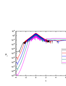
Figure 3: (Color online) Results of the numerical evolutions of the curvature perturbations with different comoving wavenumbers $k$ in non-minimal coupling matter bounce as function of cosmic time $t$. The initial values of the background parameters are the same as in Figure 1. The units of the time axis are $M_{rec}^{-1}$, the comoving wavenumber $k$ is unity for $k=m_{pl}$.

Furthermore, we calculate numerically the evolution of the particle production $\delta\phi$ with respect to $t$ and plot the result in Fig. 4. Particle production is expected in the region where the squared value of momentum scales of the perturbation modes are larger than the potential so that the WKB approximation becomes valid, such as the reheating process at the end of inflation [29]. Here at the bouncing point crossing, there is also possibilities to produce particles. In the usual case, we can define another variable $\varphi\equiv a^{\frac{3}{2}}\delta\phi$, which satisfies equation of motion as:

$$\ddot{\varphi}+\omega_{k}^{2}\varphi=...,$$ (64)

where $\omega_{k}^{2}=\frac{k^{2}}{a^{2}(t)}+m^{2}-\frac{3}{2}\dot{H}-\frac{9}{4}H^{2}$. From above we can see that, although the first two terms are positive-determined, there will remain some additional terms due to the geometry of the universe, which would cause $\omega_{k}^{2}$ to be less than zero. If this is the case, the field will have tachyonic behavior and will blow up with particle production (which can be called as tachyonic reheating [30]). However, if there is a non-minimal coupling term with a negative coupling constant $\xi$, this effect will get larger since $\omega_{k}^{2}$ gets a more negative value. This can be seen from the modified equation of motion which becomes:

$$\ddot{\varphi}+[\frac{k^{2}}{a^{2}(t)}+m^{2}-\frac{3}{2}\dot{H}-\frac{9}{4}H^{2}-\xi R]\varphi=...$$ (65)

This is usually called geometric reheating [31]. In Fig. 4 we can see that indeed the particle production gets much enhancement in the non-minimal coupling case than its minimal coupling counterparts. This is another interesting result in our case which are expected to be tested by the future experiments.

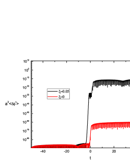
Figure 4: (Color online) Results of the numerical evolutions of the field particle production with and without non-minimal coupling term for matter bounce. The initial values of the background parameters are the same as in Figure 1.

IV conclusions and discussions

Non-minimal coupling is a very popular subject in cosmology and has been widely studied in the literature. In this paper, we have investigated the possibility of generating a matter bounce by the Lee-Wick type scalar field with a non-minimal coupling term involved, and studied its perturbations. As in the previous work done in [11], a bounce was obtained when the non-minimal coupling is not too large to have unexpected effects. However, as it gives correction to the effective mass of the field, a short period of deflation/inflation before/after the bounce will happen.

Using the standard techniques of calculating perturbations of bounce developed from previous works, we have calculated the perturbations of the model in detail. One of the big differences from previous one for minimal coupling is that the non-minimal coupling to gravity causes the difference between the two scalar perturbations $\Phi$ and $\Psi$, which will cause very interesting consequences. We have obtained the solution for each stage of evolution and compiled them together using proper matching conditions. We have found that the final dominant mode can be inherited nontrivially from the subdominant mode in the zero-th order of wave number $k$ due to this difference. This will lead to the red-tilt of the power spectrum at very large scales, which can be justified in future observation .

Another result we obtained is that due to the non-minimal coupling, the particle production of the scalar will get greatly enhanced. In the region of validity of the WKB approximation when the quantum effects become significant, the field will get excited and produce particles. This is very common in reheating process. When there is a negative effective mass squared term in the field equation, the particle production will get enhanced due to tachyonic resonance. In usual cases, the averaged value of perturbations of the scalar field will get an enhancement through bounce time due to geometrical effects. When a non-minimal coupling term is involved in the field equation, the mass of the field will be corrected. In the case of negative coupling coefficient, the field will get a more negative effective mass squared, and the particle production will get more efficiently enlarged. This is also very interesting phenomenon and can be tested by experiments on particle physics.

Finally we would like to close with some remarks on future works. The bounce with non-minimal coupling is very interesting topic since in the early epoch, Einstein’s gravity is likely to be modified, which can give some valuable effects to the evolution of our universe. It is deserved to pay attention to this project both from the theoretical side such as the perturbation, non-Gaussianity, effects on CMB and so on, and from observational side, such as the constraints, confirmation or even exclusion from experimental data. All these works are expected to take on in the future.

Appendix A Hubble parameter in Jordan and Einstein frames

This appendix is set to claim the relation between Hubble parameter in the two frames used in the text. As is well known, the differentiations of comoving time $d\eta$ are the same in the two frames, while that of cosmic time $dt$ are not. By definition, we have $d\hat{t}=\sqrt{F}dt$ where $\hat{t}$ denotes the cosmic time in Einstein frame. Due to this difference, one should be careful when using variables with derivatives in terms of $t$ such as Hubble parameter $H$. As is already mentioned in the previous sections, the Hubble parameter defined in Jordan frame is:

$$H\equiv\frac{\dot{a}}{a}=\frac{da}{adt}~{}.$$ (66)

However, we can also define a Hubble parameter in Einstein frame, which is:

$$\hat{H}\equiv\frac{\stackrel{{\scriptstyle\circ}}{{\hat{a}}}}{\hat{a}}=\frac{d\hat{a}}{\hat{a}d\hat{t}}~{},$$ (67)

where we have introduced the symbol $``\stackrel{{\scriptstyle\circ}}{{}}^{\prime\prime}$ to represent the cosmic time derivative in Einstein frame: $\stackrel{{\scriptstyle\circ}}{{}}=\frac{d}{d\hat{t}}$, $\stackrel{{\scriptstyle\circ\circ}}{{}}=\frac{d^{2}}{d\hat{t}^{2}}$, etc. We can see from the definitions that the two Hubble parameters have the same type of relation to the comoving Hubble parameters in their frames: ${\cal H}=aH$ and $\hat{\cal H}=\hat{a}\hat{H}$. Reminding the relation $\hat{a}=a\sqrt{F}$, it is easy to find the description of $\hat{H}$ in terms of $H$ and $F$:

$$\hat{H} = \frac{d(a\sqrt{F})}{aFdt}~{}$$ (68)

$$= \frac{H}{\sqrt{F}}-(\frac{1}{\sqrt{F}})\dot{}~{}.$$

Furthermore, we can derive its derivatives with respect to cosmic time $\hat{t}$ which are:

$$\stackrel{{\scriptstyle\circ}}{{\hat{H}}} = \frac{\dot{H}}{F}+H(\frac{1}{2F})\dot{}-\frac{1}{\sqrt{F}}(\frac{1}{\sqrt{F}})\ddot{}~{},$$ (69)

$$\stackrel{{\scriptstyle\circ\circ}}{{\hat{H}}} = \frac{\ddot{H}}{F\sqrt{F}}+\dot{H}(\frac{1}{F\sqrt{F}})\dot{}+\frac{H}{\sqrt{F}}(\frac{1}{2F})\ddot{}-\frac{1}{F}(\frac{1}{\sqrt{F}})^{\dddot{}}-(\frac{1}{2F})\dot{}(\frac{1}{\sqrt{F}})\ddot{}~{}.$$ (70)

Appendix B coefficients for the perturbation modes

This appendix indicates all the coefficients that appear in (62). These are calculated using the Hwang-Vishniac (Dueruelle-Mukhanov) matching conditions [7, 8]:

$${}^{(0)}G_{c}^{+}=\frac{\frac{2}{3aFt^{\frac{5}{3}}A_{c}^{+}}+B_{c}^{+}F[(\frac{20\epsilon}{9aFt^{\frac{8}{3}}}+\frac{2\dot{A_{c}^{+}}}{aFt^{\frac{5}{3}}A_{c}^{+}})H+(16\sqrt{\frac{1}{3}}\frac{\epsilon\kappa\xi\phi}{aF^{2}t^{\frac{5}{3}}}+\frac{2}{aFt^{\frac{5}{3}}}-\frac{4\epsilon}{3aFt^{\frac{5}{3}}}-\frac{4C_{c}^{+}}{aF^{2}t^{\frac{5}{3}}A_{c}^{+}})H^{2}]}{(-3B_{c}^{+}\dot{A_{c}^{+}}FH+3A_{c}^{+}\dot{B_{c}^{+}}FH+6B_{c}^{+}C_{c}^{+}H^{2}-6A_{c}^{+}E_{c}^{+}H^{2})}\Big{|}_{t_{c}}~{},$$ (71)

$${}^{(0)}K_{c}^{+}=\frac{\frac{6}{5\kappa^{2}A_{c}^{+}}-B_{c}^{+}F[\frac{18\dot{A_{c}^{+}}H}{5\kappa^{2}A_{c}^{+}}+(2.4\frac{\epsilon}{\kappa^{2}}+6.4\sqrt{3}\frac{\epsilon\xi\phi}{F\kappa}+\frac{18}{5\kappa^{2}}-\frac{36C_{c}^{+}}{5\kappa^{2}A_{c}^{+}F})H^{2}]}{(-3B_{c}^{+}\dot{A_{c}^{+}}FH+3A_{c}^{+}\dot{B_{c}^{+}}FH+6B_{c}^{+}C_{c}^{+}H^{2}-6A_{c}^{+}E_{c}^{+}H^{2})}\Big{|}_{t_{c}}~{},$$ (72)

$${}^{(1)}G_{c}^{+}=\frac{B_{c}^{+}F(\frac{4\epsilon}{9aFt^{\frac{5}{3}}}-\frac{2}{3aFt^{\frac{5}{3}}})}{(-3B_{c}^{+}\dot{A_{c}^{+}}FH+3A_{c}^{+}\dot{B_{c}^{+}}FH+6B_{c}^{+}C_{c}^{+}H^{2}-6A_{c}^{+}E_{c}^{+}H^{2})}\Big{|}_{t_{c}}~{},$$ (73)

$${}^{(1)}K_{c}^{+}=\frac{B_{c}^{+}F(\frac{4\epsilon}{5\kappa^{2}}-\frac{6}{5\kappa^{2}})}{(-3B_{c}^{+}\dot{A_{c}^{+}}FH+3A_{c}^{+}\dot{B_{c}^{+}}FH+6B_{c}^{+}C_{c}^{+}H^{2}-6A_{c}^{+}E_{c}^{+}H^{2})}\Big{|}_{t_{c}}~{},$$ (74)

$${}^{(0)}M_{c}^{+}=\frac{-A_{c}^{+}F[(\frac{20\epsilon}{9aFt^{\frac{8}{3}}}+\frac{2\dot{A_{c}^{+}}}{aFt^{\frac{5}{3}}A_{c}^{+}})H+(16\sqrt{\frac{1}{3}}\frac{\epsilon\kappa\xi\phi}{aF^{2}t^{\frac{5}{3}}}+\frac{2}{aFt^{\frac{5}{3}}}-\frac{4\epsilon}{3aFt^{\frac{5}{3}}}-\frac{4C_{c}^{+}}{aFt^{\frac{5}{3}}})H^{2}]}{(-3B_{c}^{+}\dot{A_{c}^{+}}FH+3A_{c}^{+}\dot{B_{c}^{+}}FH+6B_{c}^{+}C_{c}^{+}H^{2}-6A_{c}^{+}E_{c}^{+}H^{2})}\Big{|}_{t_{c}}~{},$$ (75)

$${}^{(0)}N_{c}^{+}=\frac{A_{c}^{+}F[\frac{18\dot{A_{c}^{+}}H}{5\kappa^{2}A_{c}^{+}}-(2.4\frac{\epsilon}{\kappa^{2}}+6.4\sqrt{3}\frac{\epsilon\xi\phi}{F\kappa}-\frac{18}{5\kappa^{2}}+\frac{36C_{c}^{+}}{5\kappa^{2}A_{c}^{+}F})H^{2}]}{(-3B_{c}^{+}\dot{A_{c}^{+}}FH+3A_{c}^{+}\dot{B_{c}^{+}}FH+6B_{c}^{+}C_{c}^{+}H^{2}-6A_{c}^{+}E_{c}^{+}H^{2})}\Big{|}_{t_{c}}~{},$$ (76)

$${}^{(1)}M_{c}^{+}=\frac{A_{c}^{+}F(\frac{4\epsilon}{9aFt^{\frac{5}{3}}}-\frac{2}{3aFt^{\frac{5}{3}}})}{(-3B_{c}^{+}\dot{A_{c}^{+}}FH+3A_{c}^{+}\dot{B_{c}^{+}}FH+6B_{c}^{+}C_{c}^{+}H^{2}-6A_{c}^{+}E_{c}^{+}H^{2})}\Big{|}_{t_{c}}~{},$$ (77)

$${}^{(1)}N_{c}^{+}=\frac{A_{c}^{+}F(\frac{4\epsilon}{5\kappa^{2}}-\frac{6}{5\kappa^{2}})}{(-3B_{c}^{+}\dot{A_{c}^{+}}FH+3A_{c}^{+}\dot{B_{c}^{+}}FH+6B_{c}^{+}C_{c}^{+}H^{2}-6A_{c}^{+}E_{c}^{+}H^{2})}\Big{|}_{t_{c}}~{},$$ (78)

$${}^{(0)}M_{e}^{+}=\frac{\kappa^{2}(2\dot{A_{e}^{-}}Ft^{\frac{8}{3}}-4C_{e}^{-}Ht^{\frac{8}{3}}+\frac{20}{9}t^{\frac{5}{3}}\epsilon A_{e}^{-}F+2A_{e}^{-}HFt^{\frac{8}{3}}-\frac{4}{3}\epsilon A_{e}^{-}HFt^{\frac{8}{3}}+8A_{e}^{-}\kappa^{2}\xi\phi Ht^{\frac{8}{3}}\epsilon\sqrt{\frac{4}{3\kappa^{2}}})}{\epsilon(\frac{8}{3}Ft^{\frac{5}{3}}+16\kappa^{2}\xi\phi Ht^{\frac{8}{3}}\sqrt{\frac{4}{3\kappa^{2}}})}\Big{|}_{t_{e}}~{},$$ (79)

$${}^{(0)}N_{e}^{+}=\frac{\kappa^{2}(2\dot{B_{e}^{-}}Ft^{\frac{8}{3}}-4E_{e}^{-}Ht^{\frac{8}{3}}+\frac{20}{9}t^{\frac{5}{3}}\epsilon B_{e}^{-}F+2B_{e}^{-}HFt^{\frac{8}{3}}-\frac{4}{3}\epsilon B_{e}^{-}HFt^{\frac{8}{3}}+8B_{e}^{-}\kappa^{2}\xi\phi Ht^{\frac{8}{3}}\epsilon\sqrt{\frac{4}{3\kappa^{2}}})}{\epsilon(\frac{8}{3}Ft^{\frac{5}{3}}+16\kappa^{2}\xi\phi Ht^{\frac{8}{3}}\sqrt{\frac{4}{3\kappa^{2}}})}\Big{|}_{t_{e}}~{},$$ (80)

$${}^{(1)}M_{e}^{+}=\frac{\kappa^{2}Ft{}^{\frac{8}{3}}(-\frac{2}{3}+\frac{4}{9}\epsilon)A_{e}^{-}}{H\epsilon(\frac{8}{3}Ft^{\frac{5}{3}}+16\kappa^{2}\xi\phi Ht^{\frac{8}{3}}\sqrt{\frac{4}{3\kappa^{2}}})}\Big{|}_{t_{e}}~{},$$ (81)

$${}^{(1)}N_{e}^{+}=\frac{\kappa^{2}Ft{}^{\frac{8}{3}}(-\frac{2}{3}+\frac{4}{9}\epsilon)B_{e}^{-}}{H\epsilon(\frac{8}{3}Ft^{\frac{5}{3}}+16\kappa^{2}\xi\phi Ht^{\frac{8}{3}}\sqrt{\frac{4}{3\kappa^{2}}})}\Big{|}_{t_{e}}~{},$$ (82)

where

$$A_{c}^{+}=\frac{1}{a_{1}\epsilon(t-t_{\ast})^{1+\frac{1}{\epsilon}}[1-\frac{4\xi\phi_{0}}{3}(\ln{(t-t_{\ast})})^{2}]}~{},~{}B_{c}^{+}=\frac{2\epsilon}{\kappa^{2}}\Bigl{(}\frac{1}{1+\epsilon}+\frac{8\xi\phi_{0}[\epsilon-(1+\epsilon)\ln{(t-t_{\ast})}]}{3(1+\epsilon)^{3}[1-\frac{4\xi\phi_{0}}{3}(\ln{(t-t_{\ast})})^{2}]}\Bigr{)}~{},$$ (83)

$$C_{c}^{+}=\frac{\frac{4}{\sqrt{3\kappa^{2}}}\kappa^{2}\xi\phi}{a_{1}(t-t_{\ast})^{1+\frac{1}{\epsilon}}[1-\frac{4\xi\phi_{0}}{3}(\ln{(t-t_{\ast})})^{2}]}~{},$$ (84)

$$E_{c}^{+}=-\frac{8\epsilon\xi\phi\{(1+\epsilon)^{2}[1-\frac{4\xi\phi_{0}}{3}(\ln{(t-t_{\ast})})^{2}]-\frac{8\epsilon\xi\phi_{0}}{3}[\epsilon+(1+\epsilon)\ln{(t-t_{\ast})}]\}}{\sqrt{3\kappa^{2}}(1+\epsilon)^{3}[1-\frac{4\xi\phi_{0}}{3}(\ln{(t-t_{\ast})})^{2}]}~{},$$ (85)

$$A_{e}^{-}=\frac{1}{a_{2}\epsilon(t-t_{{\dagger}})^{1+\frac{1}{\epsilon}}[1-\frac{4\xi\phi_{0}}{3}(\ln{(t-t_{{\dagger}})})^{2}]}~{},~{}B_{e}^{-}=\frac{2\epsilon}{\kappa^{2}}\Bigl{(}\frac{1}{1+\epsilon}+\frac{8\xi\phi_{0}[\epsilon-(1+\epsilon)\ln{(t-t_{{\dagger}})}]}{3(1+\epsilon)^{3}[1-\frac{4\xi\phi_{0}}{3}(\ln{(t-t_{{\dagger}})})^{2}]}\Bigr{)}~{},$$ (86)

$$C_{e}^{-}=\frac{\frac{4}{\sqrt{3\kappa^{2}}}\kappa^{2}\xi\phi}{a_{2}(t-t_{{\dagger}})^{1+\frac{1}{\epsilon}}[1-\frac{4\xi\phi_{0}}{3}(\ln{(t-t_{{\dagger}})})^{2}]}~{},$$ (87)

$$E_{e}^{-}=-\frac{8\epsilon\xi\phi\{(1+\epsilon)^{2}[1-\frac{4\xi\phi_{0}}{3}(\ln{(t-t_{{\dagger}})})^{2}]-\frac{8\epsilon\xi\phi_{0}}{3}[\epsilon+(1+\epsilon)\ln{(t-t_{{\dagger}})}]\}}{\sqrt{3\kappa^{2}}(1+\epsilon)^{3}[1-\frac{4\xi\phi_{0}}{3}(\ln{(t-t_{{\dagger}})})^{2}]}~{}.$$ (88)

The constants $t_{\ast}$ and $t_{\dagger}$ are set to guarantee the continuity of $H$ at the joint point $t_{c}$ and $t_{e}$, and one can straightforwardly check that in the limit of $\xi=0$, we have ${}^{(0)}M_{c}^{+}$ and ${}^{(0)}M_{e}^{+}$=0, and a scale-invariant power spectrum can be obtained for the whole region of large scales.

References

• [1] V. F. Mukhanov and R. H. Brandenberger, Phys. Rev. Lett.  68, 1969 (1992); R. H. Brandenberger, V. F. Mukhanov and A. Sornborger, Phys. Rev.  D 48, 1629 (1993); For recent review see M. Novello and S. E. P. Bergliaffa, Phys. Rept.  463, 127 (2008).
• [2] A. H. Guth, Phys. Rev.  D 23, 347 (1981); A. Albrecht and P. J. Steinhardt, Phys. Rev. Lett.  48, 1220 (1982); A. D. Linde, Phys. Lett.  B 108, 389 (1982).
• [3] S. W. Hawking, and G. F. R. Ellis, The large scale structure of space-time, Cambridge University Press (1973); A. Borde and A. Vilenkin, Phys. Rev. Lett.  72, 3305 (1994).
• [4] A. Borde and A. Vilenkin, Phys. Rev. Lett.  72, 3305 (1994).
• [5] J. Martin and R. H. Brandenberger, Phys. Rev.  D 63, 123501 (2001); R. H. Brandenberger and J. Martin, Mod. Phys. Lett.  A 16, 999 (2001).
• [6] For calculations of perturbations in a bounce scenario, we draw readers’ attentions to e. g. D. Wands, Phys. Rev.  D 60, 023507 (1999); P. Peter and N. Pinto-Neto, Phys. Rev.  D 66, 063509 (2002); F. Finelli, JCAP 0310, 011 (2003); L. E. Allen and D. Wands, Phys. Rev.  D 70, 063515 (2004); F. Finelli, P. Peter and N. Pinto-Neto, Phys. Rev.  D 77, 103508 (2008); A. Cardoso and D. Wands, Phys. Rev.  D 77, 123538 (2008).
• [7] J. c. Hwang and E. T. Vishniac, Astrophys. J.  382, 363 (1991).
• [8] N. Deruelle and V. F. Mukhanov, Phys. Rev.  D 52, 5549 (1995).
• [9] Y. F. Cai and E. N. Saridakis, JCAP 0910, 020 (2009); K. i. I. Maeda, Y. Misonoh and T. Kobayashi, arXiv:1006.2739 [hep-th].
• [10] Y. F. Cai and X. Zhang, JCAP 0906, 003 (2009); Y. F. Cai, W. Xue, R. Brandenberger and X. Zhang, JCAP 0905, 011 (2009).
• [11] Y. F. Cai, T. t. Qiu, R. Brandenberger and X. m. Zhang, Phys. Rev. D 80, 023511 (2009).
• [12] N. A. Chernikov and E. A. Tagirov, Annales Poincare Phys. Theor. A 9 (1968) 109; C. G. . Callan, S. R. Coleman and R. Jackiw, Annals Phys. 59 (1970) 42; N. D. Birrell and P. C. W. Davies, Quantum Fields In Curved Space, Cambridge University Press (1982).
• [13] Y. Fujii and K. Maeda, The Scalar-Tensor Theory of Gravitation,” Cambridge University Press (2003); B. Boisseau, G. Esposito-Farese, D. Polarski and A. A. Starobinsky, Phys. Rev. Lett.  85, 2236 (2000).
• [14] C. Brans and R. H. Dicke, Phys. Rev.  124, 925 (1961).
• [15] M. Gasperini and G. Veneziano, Astropart. Phys.  1, 317 (1993); M. Gasperini and G. Veneziano, Phys. Rept.  373, 1 (2003).
• [16] S. Nojiri, S. D. Odintsov and M. Sasaki, Phys. Rev.  D 71, 123509 (2005) and the following literature.
• [17] T. P. Sotiriou and V. Faraoni, Rev. Mod. Phys.  82, 451 (2010); A. De Felice and S. Tsujikawa, Living Rev. Rel.  13, 3 (2010); A. De Felice and S. Tsujikawa, arXiv:1005.0868 [astro-ph.CO].
• [18] M. R. Setare, J. Sadeghi and A. Banijamali, Phys. Lett.  B 669, 9 (2008); J. Sadeghi, M. R. Setare, A. R. Amani and S. M. Noorbakhsh, Phys. Lett.  B 685, 229 (2010); T. Qiu, arXiv:1007.2929 [hep-ph].
• [19] V. Faraoni, Phys. Rev.  D 53, 6813 (1996).
• [20] V. Faraoni, Phys. Rev.  D 62, 023504 (2000); S. Nojiri and S. D. Odintsov, eConf C0602061, 06 (2006) [Int. J. Geom. Meth. Mod. Phys. 4, 115 (2007)]; M. R. Setare and E. N. Saridakis, Phys. Lett.  B 671, 331 (2009).
• [21] B. Feng, X. L. Wang and X. M. Zhang, Phys. Lett.  B 607, 35 (2005); M. z. Li, B. Feng and X. m. Zhang, JCAP 0512, 002 (2005). See also Y. F. Cai, E. N. Saridakis, M. R. Setare and J. Q. Xia, arXiv:0909.2776 [hep-th]; T. Qiu, Mod. Phys. Lett.  A 25, 909 (2010) for reviews.
• [22] T. D. Lee and G. C. Wick, Nucl. Phys.  B 9, 209 (1969); T. D. Lee and G. C. Wick, Phys. Rev.  D 2, 1033 (1970).
• [23] B. Grinstein, D. O’Connell and M. B. Wise, Phys. Rev.  D 77, 025012 (2008).
• [24] A. van Tonder, arXiv:0810.1928 [hep-th].
• [25] S. M. Carroll, M. Hoffman and M. Trodden, Phys. Rev.  D 68, 023509 (2003); J. M. Cline, S. Jeon and G. D. Moore, Phys. Rev.  D 70, 043543 (2004).
• [26] J. Karouby and R. Brandenberger, arXiv:1004.4947 [hep-th].
• [27] V. F. Mukhanov, H. A. Feldman and R. H. Brandenberger, Phys. Rept. 215, 203 (1992).
• [28] Y. F. Cai, T. Qiu, R. Brandenberger, Y. S. Piao and X. Zhang, JCAP 0803, 013 (2008).
• [29] A. Albrecht, P. J. Steinhardt, M. S. Turner and F. Wilczek, Phys. Rev. Lett. 48, 1437 (1982); A. D. Dolgov and A. D. Linde, Phys. Lett.  B 116, 329 (1982); L. F. Abbott, E. Farhi and M. B. Wise, Phys. Lett.  B 117, 29 (1982); J. H. Traschen and R. H. Brandenberger, Phys. Rev.  D 42, 2491 (1990); L. Kofman, A. D. Linde and A. A. Starobinsky, Phys. Rev. Lett. 73, 3195 (1994); Y. Shtanov, J. H. Traschen and R. H. Brandenberger, Phys. Rev. D 51, 5438 (1995); L. Kofman, A. D. Linde and A. A. Starobinsky, Phys. Rev.  D 56, 3258 (1997). For comprehensive reviews see B. A. Bassett, S. Tsujikawa and D. Wands, Rev. Mod. Phys. 78, 537 (2006); R. Allahverdi, R. Brandenberger, F. Y. Cyr-Racine and A. Mazumdar, arXiv:1001.2600 [hep-th].
• [30] P. B. Greene, L. Kofman and A. A. Starobinsky, Nucl. Phys.  B 543, 423 (1999); G. N. Felder, J. Garcia-Bellido, P. B. Greene, L. Kofman, A. D. Linde and I. Tkachev, Phys. Rev. Lett.  87, 011601 (2001).
• [31] B. A. Bassett and S. Liberati, Phys. Rev.  D 58, 021302 (1998) [Erratum-ibid. D 60, 049902 (1999)]; S. Tsujikawa, K. i. Maeda and T. Torii, Phys. Rev.  D 61, 103501 (2000); S. Tsujikawa and B. A. Bassett, Phys. Rev.  D 62, 043510 (2000); B. A. Bassett, S. Tsujikawa and D. Wands, Rev. Mod. Phys. 78, 537 (2006).
• [32] J. Martin and P. Peter, Phys. Rev. Lett.  92, 061301 (2004).