Relaxation in quantum systems. Manifestation of the state-selective reactive decay

Abstract

The effect of state-selective reactive decay on the relaxation kinetics of quantum multistate systems is studied in detail in the Bloch-Redfield approach (BRA). The results are applied to the analysis of this effect in radical pair recombination kinetics. The BRA is shown to be able to describe quantitatively most important specific features of the recombination kinetics including those predicted by phenomenological treatment and by recently proposed approaches based on quantum measurement theories.

I Introduction

Recently some attention has been attracted to the discussion of theoretical approaches for describing the effect of state-selective reaction on the reactive quantum systems. The most popular example of such processes is spin-selective condensed phase physicochemical reactions of paramagnetic particles.St The interest in this problem is inspired by new ideas, known in the quantum measurement theory,Brag ; Niel which can probably be useful in the analysis of relaxation in quantum systems.Hor ; Kom At first glance, these ideas really provide some new insight into the specific features of kinetics of state selective processes. In support of this conclusion recently some results have been presented,Gau ; Hor ; Kom which seem to demonstrate some new possibilities of the new methods for treating experimental results.

The discussion of these methods stems from some seeming limitations of the traditional approach looking rather heuristic. The main point of this approach is considered to be the description of spin-selective reactivity.Hab The description is based on the simple model for the reactivity supermatrix $\hat{K}$ operating on the spin density matrix of the system $\rho$. In this model, as applied to radical pair (RP) recombination with the rates $\kappa_{S}$ and $\kappa_{T}$ in the singlet ($S$) and triplet ($T$) states, respectively,

$$\hat{K}\rho=\mbox{$\frac{1}{2}$}\big{\{}\kappa_{S}[P_{S},\rho]_{+}+\kappa_{T}[P_{T},\rho]_{+}\big{\}}$$ (1)

where $P_{S}$ and $P_{T}$ are the operators of projection on the $S$ and $T$ states, respectively, and $[P,\rho]_{+}=P\rho+\rho P$. The analysis based on the quantum measurement approach shows Hor ; Kom that the expression (1) leads to the experimentally distinguishable underestimation the dephasing effect of reactivity.

In this short paper we will analyze the state-selective reactivity effects on the relaxation in quantum systems within the (traditional) Bloch-Redfield approach (BRA).Blo ; Red ; Hbr ; Abr The BRA is the basic approach in the magnetic relaxation theory, but, in principle, it is very general and under quite realistic assumptions can properly describe a large variety of quantum relaxation processes.

The results of our work demonstrate that formula of type of eq. (1) is directly follows from the BRA. It is, first, derived for the simple three-state system (THSS), in which relaxation in the two state system is induced by reactive transitions to the third state, and then obtained [just in the form of eq. (1)] as applied to the case of spin selective RP recombination, by treating the reaction as spin-dependent transitions from excited (electronic) $S$ and $T$ states of the RP to the ground state.

It is also shown that the BRA enables one to essentially generalize eq. (1) by taking into account possible additional $ST$ dephasing, accompanying the reaction. The generalized formula appears to be able to describe all predictions of the quantum measurement approach, discussed in refs. [4,5], under some assumptions on relative value of reaction and dephasing rates. The effect of the interradical-distance dependent reactivity and exchange interaction is also briefly analyzed within the approach based on the stochastic Liouville equation Fre ; Shu1 which allows one to rigorously describe the manifestation of relative diffusion of radicals.

II General formulas

Here we briefly discuss the main points of the BRA which are important for our further analysis of relaxation kinetics.Hbr ; Alek For convenience, in our discussion we will use the frequency units for energies (i.e. $\hbar=1$) and the notation $\beta=1/(k_{B}T)$.

In the BRA the evolution of the system is described by the Liouville equation for the density matrix $\rho(t)$:Fre ; Shu1

$$\dot{\rho}=-i[H_{s},\rho]+\hat{R}\rho,\;\;\mbox{with}\;\;[H_{s},\rho]=H_{s}\rho-\rho H_{s}.$$ (2)

in which $H_{s}$ is the non-fluctuating part of the Hamiltonian $H$ of the system and $\hat{R}$ is the relaxation supermatrix (the matrix in the Liouville space of matrix elements of the density matrix). Thus, the problem of description of the relaxation kinetics reduces to the evaluation of the matrix $\hat{R}$ and subsequent solution of eq. (2).

For the system in a bath the HamiltonianHbr ; Alek

$$H=H_{s}+H_{sl}+H_{l},$$ (3)

where $H_{l}$ is the Hamiltonian of the bath whose specific form is not important for our further analysis. The term

$$H_{sl}=\sum\nolimits_{n}\!\Phi_{n}({\bf q})\Lambda_{n}$$ (4)

represents the interaction of the system with the bath, in which $\Lambda_{n}$ are the Hermitian operators in the space of the system ($|\nu\rangle,\,\nu=0,1,2$) and $\Phi_{n}(\bf{q})$ are the lattice coordinate dependent Hermitian operators of fluctuating amplitudes of interaction (see below).

In what follows it will be convenient to represent operators $\Lambda_{n}$ as sums of those $\Lambda_{n}^{r}$, defined byHbr ; Alek

$$\Lambda_{n}(t)=e^{iH_{s}t}\Lambda_{n}e^{-iH_{s}t}=\sum\nolimits_{r}\!\Lambda_{n}^{r}e^{i\omega_{n}^{r}t},$$ (5)

which describe transitions between different pairs of states of $H_{s}$ [$\Lambda_{n}\equiv\Lambda_{n}(t=0)=\sum\nolimits_{r}\!\Lambda_{n}^{r}$].

In the sum (5) the frequencies $\omega_{n}^{r}$ are the differences of eigenstates $\nu_{j}$ of the Hamiltonian $H_{s}$ corresponding to eigenstates $|j\rangle$ (i.e. $H_{s}|j\rangle=\nu_{j}|j\rangle$):

$$\omega_{n}^{r}=\nu_{j}-\nu_{j^{\prime}}=\omega_{jj^{\prime}}$$ (6)

and the operators $\Lambda_{n}^{r}$ are defined by

$$\Lambda_{n}^{r}=\langle j|\Lambda_{n}|j^{\prime}\rangle\delta_{\omega_{n}^{r},\omega_{jj^{\prime}}}.$$ (7)

The operators and frequencies in eq. (5) satisfy the relations $(\Lambda_{n}^{r})^{{\dagger}}=\Lambda_{n}^{-r}$ and $\omega_{n}^{-r}=-\omega_{n}^{r}$ (see examples below).Hbr ; Alek

In the BRA the relaxation rates are determined by the pair correlation functionsHbr ; Alek

$$K_{nn^{\prime}}^{+}(t)=\langle\Phi_{n}(t)\Phi_{n^{\prime}}\rangle,\;\;K_{nn^{\prime}}^{-}(t)=\langle\Phi_{n}\Phi_{n^{\prime}}(t)\rangle,$$ (8)

in which

$$\Phi_{n}(t)=e^{iH_{l}t}\Phi_{n}e^{-iH_{l}t}$$ (9)

and the averages $\langle\dots\rangle$ are evaluated over the equilibrium lattice density matrix $\rho_{l}$:

$$\langle A\rangle={\rm Tr}(\rho_{l}A)\;\;\mbox{with}\;\;\rho_{l}=e^{-\beta H_{l}}/{\rm Tr}(e^{-\beta H_{l}}).$$ (10)

In addition we will introduce their Fourier transforms

$$J^{\pm}_{nn^{\prime}}(\omega)=\int_{-\infty}^{\infty}\!dt\,K_{nn^{\prime}}^{\pm}(t)e^{i\omega t}$$ (11)

for which we get $J_{nn^{\prime}}^{+}(\omega)=e^{\beta\omega}J_{n^{\prime}n}^{-}(\omega)=e^{\beta\omega}J_{n^{\prime}n}^{+}(-\omega).$

The most important BRA results are conveniently expressed in terms of Fourier transforms

$$J_{nn^{\prime}}(\omega)=\mbox{$\frac{1}{2}$}[J_{nn^{\prime}}^{+}(\omega)+J_{n^{\prime}n}^{-}(\omega)]$$ (12)

of symmetrized functions $K_{nn^{\prime}}(t)=\mbox{$\frac{1}{2}$}[K_{nn^{\prime}}^{+}(t)+K_{n^{\prime}n}^{-}(t)]$.

In particular, the supermatrix $\hat{R}$ is given byHbr ; Alek

$$\hat{R}=\mbox{$\frac{1}{2}$}(\hat{R}_{1}+\hat{R}_{2}),$$ (13)

where

$$\hat{R}_{1}\rho\! = \!\!\!\sum_{nn^{\prime}r}\!J_{n^{\prime}n}(\omega_{n}^{r})\Big{[}\big{[}\Lambda_{n^{\prime}}^{r},\rho\big{]},\Lambda_{n}\Big{]},$$ (14)

$$\hat{R}_{2}\rho\! = \!\!\!\sum_{nn^{\prime}r}\!J_{n^{\prime}n}(\omega_{n}^{r})\tanh(\mbox{$\frac{1}{2}$}\beta\omega_{n^{\prime}}^{r})\Big{[}\Lambda_{n},\big{[}\Lambda_{n^{\prime}}^{r},\rho\big{]}_{+}\Big{]},\qquad\;$$ (15)

with $\big{[}\Lambda,\rho\big{]}=\Lambda\rho-\rho\Lambda\;\;\mbox{and}\;\;\big{[}\Lambda,\rho\big{]}_{+}=\Lambda\rho+\rho\Lambda.$

Strictly speaking, in addition to relaxation the BRA also predicts some frequency shifts,Blo ; Red ; Hbr ; Abr though, we are not going to analyze them in this work.

Concluding the short review of the BRA we recall the conditions of validity of this approach. The most important is the condition $\tau_{c}\ll\|\hat{R}\|$Blo ; Red ; Hbr ; Abr in which $\tau_{c}$ is the characteristic correlation time of $H_{sl}$ fluctuations, i.e.the average time of decay of correlation functions $K_{nn^{\prime}}^{\pm}(t)$. This condition insures the validity of the second order perturbation approximation used in the derivation of the kinetic equation (2). Some additional condition is also required which ensures fast thermalization of the lattice, and in particular, fast relaxation of the non-diagonal diagonal elements between $s$ and $l$ systems generated by the interaction $H_{sl}$.Alek This additional condition is, in reality, not very restrictiveAlek and we are not going to discuss it in this work.

III Three-state system

In this Section we will demonstrate the effect of reactivity on the quantum evolution kinetics by the example of the relaxation in the simple THSS, schematically shown in Fig. 1a. The THSS consists of the subsystem of two states $(|0\rangle,|1\rangle)$ and the third state $|2\rangle$, transition to which model the reaction. In the analysis we will also take into account the additional $0\!-\!1$ dephasing [because of possible fluctuations of $0\!-\!1$ splitting (see Sec. III.C.)], but, first, we will neglect this effect.

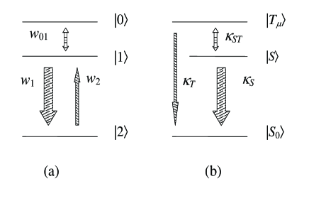
Figure 1: The schematic picture of the levels and transitions between these levels for: (a) the three-state system ($w_{1}$ and $w_{2}$ are the rates of population relaxation, and $w_{01}$ is the $0\!-\!1$ dephasing rate) and (b) radical pair ($\kappa_{S}$ and $\kappa_{T}$ are the reaction rates, and $\kappa_{ST}$ is the $ST_{\mu}$ dephasing rate,  ($\mu=0,\pm$).

In the considered THSS the terms of the total Hamiltonian $H$ [eq. (3)] are defined as follows

$$H_{s} = \omega_{0}|0\rangle\langle 0|+\mbox{$\frac{1}{2}$}\omega_{s}(|1\rangle\langle 1|-|2\rangle\langle 2|),$$ (16)

$$H_{sl} = H_{sl}(12)=\mbox{$\frac{1}{2}$}\!\sum\nolimits_{n=x,y}\!\!\Phi_{n}({\bf q})\sigma_{n}.$$ (17)

In the operator $H_{sl}$, representing (fluctuating) interaction between $|1\rangle$ and $|2\rangle$ states, in which $\sigma_{n},\,(n=x,y),\,$ are the Pauli matrices in the space ($|1\rangle,|2\rangle$): $\sigma_{x}=|1\rangle\langle 2|+|2\rangle\langle 1|$ and $\sigma_{y}=i(|2\rangle\langle 1|-|1\rangle\langle 2|)$ . In principle, $H_{sl}$ can be treated as the interaction of a quasispin, associated with matrices $\sigma_{x,y}$, with the fluctuating magnetic field, whose components are $\Phi_{n}({\bf q}),\,(n=x,y)$.

Formulas (16) and (17) present the most general form of the two-state Hamiltonian in the absence fluctuating diagonal interaction. As for the lattice coordinate dependent (fluctuating) components $\Phi_{n}({\bf q})$, their particular forms are not of real importance for our further analysis.

The operators $\Lambda_{n}^{r}$ introduced in formula (5) are written as

$$\Lambda_{x}^{1}\;\; = \;\>i\Lambda_{y}^{1}\;\;=\mbox{$\frac{1}{4}$}(\sigma_{x}+i\sigma_{y})=\mbox{$\frac{1}{2}$}|1\rangle\langle 2|,$$ (18)

$$\Lambda_{x}^{-1} = \!\!-i\Lambda_{y}^{-1}=\mbox{$\frac{1}{4}$}(\sigma_{y}-i\sigma_{x})=\mbox{$\frac{1}{2}$}|2\rangle\langle 1|$$ (19)

As for fluctuations of $\Phi_{n}$, for simplicity, they are suggested to be uncorrelated and axially symmetric, i.e.

$$J_{nn^{\prime}}(\omega)=J(\omega)\delta_{nn^{\prime}},\;\;(n,n^{\prime}=x,y).$$ (20)

III.1 Relaxation kinetics in two-state $(1,2)$ subsystem

First of all, it is clear that in the absence of interaction between the state $|0\rangle$ and two states $|1\rangle,|2\rangle$ the relaxation in the subsystem of two states $|1\rangle,|2\rangle$ is described by the conventional Bloch equations for the density matrix $\rho$ in the subspace $\{|1\rangle,|2\rangle\}$:Alek

$$\dot{\rho}_{11} = -w_{11}\rho_{11}+w_{22}\rho_{22}$$ (21)

$$\dot{\rho}_{22} = -w_{22}\rho_{22}+w_{11}\rho_{11}$$ (22)

$$\dot{\rho}_{\mu} = -w_{n}\rho_{\mu},\qquad(\mu=12,\,21).$$ (23)

The rates are given by

$$w_{11} = e^{\beta\omega_{s}}w_{22}=J(\omega_{s})/(1+e^{-\beta\omega_{s}}),$$ (24)

$$w_{n} = w_{12}=\mbox{$\frac{1}{2}$}(w_{11}+w_{22})=\mbox{$\frac{1}{2}$}J(\omega_{s}).$$ (25)

In particular, for large splitting $\omega_{0}\gg\beta^{-1}$

$$w_{11}=w_{11}^{\infty}=J(\omega_{s}),\;\;w_{22}=0,\;\;w_{n}=\mbox{$\frac{1}{2}$}w_{11}.$$ (26)

III.2 Relaxation kinetics in three-state system

The analysis within the THSS shows that, in addition to relaxation in $(|1\rangle,|2\rangle)$-subspace, the fluctuating interaction $H_{sl}$ induces also the relaxation of $0\!-\!1$ and $0\!-\!2$ phases, i.e. the decay of non-diagonal elements $\rho_{0\mu}$ and $\rho_{\mu 0}$ with $\mu=1,2$.

The expressions for corresponding phase relaxation can straightforwardly be derived with the use of eqs. (13) and (14).

For example, the decay rate of $\rho_{01}$ is determined by the matrix elements

$$\langle 0|\hat{R}_{1}\rho|1\rangle=J(\omega_{s})\langle 1|\Lambda_{xy}^{0}|1\rangle\rho_{01}=-\mbox{$\frac{1}{2}$}J(\omega_{s})\rho_{01},$$ (27)

and

$$\langle 0|\hat{R}_{2}\rho|1\rangle = J(\omega_{s})\tanh(\mbox{$\frac{1}{2}$}\beta\omega_{s})\langle 1|\Lambda_{xy}^{0}|1\rangle\rho_{01}$$ (28)

$$= -\mbox{$\frac{1}{2}$}J(\omega_{s})\tanh(\mbox{$\frac{1}{2}$}\beta\omega_{s})\rho_{01}$$

where

$$\Lambda_{xy}^{0}=\Lambda_{x}^{1}\Lambda_{x}^{-1}+\Lambda_{y}^{1}\Lambda_{y}^{-1}.$$ (29)

Similar formulas can be obtained for $\langle 1|\hat{R}_{j}\rho|0\rangle$ elements. Substitution of expressions (27) and (28) into eq. (13) yields simple kinetic equations

$$\dot{\rho}_{\mu\mu^{\prime}}=-w_{01}\rho_{\mu\mu^{\prime}},\;\;\mbox{with}\;\;\mu\mu^{\prime}=01,10.$$ (30)

describing the exponential $0\!-\!1$ dephasing with the rate

$$w_{01}=\mbox{$\frac{1}{2}$}w_{11}=\mbox{$\frac{1}{2}$}J(\omega_{s})(1+e^{-\beta\omega_{s}})^{-1}.$$ (31)

The analogous consideration enables one to derived the kinetic equations for relaxation of $0\!-\!2$ phases:

$$\dot{\rho}_{\mu\mu^{\prime}}=-w_{02}\rho_{\mu\mu^{\prime}},\;\;\mbox{with}\;\;\mu\mu^{\prime}=02,20,$$ (32)

where

$$w_{02}=\mbox{$\frac{1}{2}$}w_{22}=\mbox{$\frac{1}{2}$}J(\omega_{s})(1+e^{\beta\omega_{s}})^{-1}.$$ (33)

It is important to note that in the case of irreversible $1\to 2$ relaxation transitions, corresponding to the limit $\beta\omega_{s}\to\infty$, the obtained kinetic equations can be represented in a simple matrix form with the use of the operator $P_{1}=|1\rangle\langle 1|$ of projection onto the reactive state $|1\rangle$:

$$\dot{\rho}=-\mbox{$\frac{1}{2}$}w_{11}^{\infty}[P_{1},\rho]_{+},$$ (34)

with $w_{11}^{\infty}$ defined in eq. (26) and $[P_{1},\rho]_{+}=P_{1}\rho+\rho P_{1}$. It is easily seen that eq. (34) correctly describes relaxation not only of the diagonal elements of the density matrix (population relaxation) but also of all non-diagonal elements (phase relaxation).

Naturally, the effect of additional irreversible relaxation transitions $0\to 2$ with the rate $w_{00}^{\infty}$, can also be described, but with the more general equation $\dot{\rho}=-\mbox{$\frac{1}{2}$}(w_{11}^{\infty}[P_{1},\rho]_{+}+w_{00}^{\infty}[P_{0},\rho]_{+}),$ with $P_{0}=|0\rangle\langle 0|$. Of course this equation predicts additional dephasing in the system of type of that considered above.

Note that similar expression, can be written for reversible transitions (in the case of finite $\beta\omega_{s}$). One should only add the terms proportional to $P_{2}=|2\rangle\langle 2|$ and the operator describing $1\!-\!2$ (or $0\!-\!2$) relaxation.

III.3 Effect of splitting fluctuations

In the above analysis we have not taken into account possible fluctuating interactions diagonal in the bases $(|0\rangle,|1\rangle,|2\rangle)$ (the diagonal contributions to $H_{sl}$).

In the two state system considered above (see Sec. IIIA) the effect of the fluctuating diagonal interaction of type of $\mbox{$\frac{1}{2}$}\Phi_{z}({\bf q})\sigma_{z}$ is known to reduce to additional dephasing.Blo ; Hbr ; Abr ; Alek

In particular, in the simple case of isotropic fluctuating interaction $\{\Phi_{n}\}$, $(n=x,y,z)$, resulting in the interaction $H_{sl}=\mbox{$\frac{1}{2}$}\!\sum_{n=x,y,z}\!\Phi_{n}({\bf q})\sigma_{n}$, i.e. for $J_{nn^{\prime}}(\omega)=J(\omega)\delta_{nn^{\prime}},\;\;(n,n^{\prime}=x,y,z)$, the dephasing rate $w_{n}=w_{12}$ is represented as Abr ; Alek

$$w_{n}=\mbox{$\frac{1}{2}$}({\bar{w}}_{n}+w_{11}),\;\;\mbox{with}\;\;{\bar{w}}_{n}=J(0).$$ (35)

Comparison of this formula with eq. (25) shows that the above-mentioned additional dephasing manifests itself in the contribution $\mbox{$\frac{1}{2}$}w_{n}^{0}=\mbox{$\frac{1}{2}$}J(0)$ to the dephasing rate.

Naturally, similar effect is predicted in the presence of the additional fluctuating diagonal interaction, changing $(0-1)$ splitting:

$$H_{sl}(01)=\mbox{$\frac{1}{2}$}(|0\rangle\langle 0|-|1\rangle\langle 1|)\Phi_{01}({\bf q}).$$ (36)

Assuming uncorrelated fluctuations of $\Phi_{01}$ and the field components $\Phi_{n}$ [see eq. (17)] one obtains for the rate of $0\!\!-\!\!1$ dephasing

$$w_{01}=\mbox{$\frac{1}{2}$}({\bar{w}}_{01}+w_{11}),\;\;\mbox{where}\;\;{\bar{w}}_{01}=J_{01}(0).$$ (37)

The Fourier transformed correlation function $J_{01}(\omega)$ can be calculated by substituting $\Phi_{01}({\bf q})$ into eqs. (8)-(12).

Similar expression can be derived for the rate of $0\!\!-\!\!2$ dephasing caused by the additional fluctuating diagonal interaction, changing $(0-2)$ splitting.

As in the absence splitting fluctuations, considered above, the obtained relaxation equations are conveniently combined into matrix equation which in the irreversible relaxation limit $\beta\omega_{s}\to\infty$ is expressed in the form

$$\dot{\rho}=-\mbox{$\frac{1}{2}$}\{w_{11}^{\infty}[P_{1},\rho]_{+}+{\bar{w}}_{01}\hat{\cal P}_{1}(\rho)\}.$$ (38)

where

$$\hat{\cal P}_{1}(\rho)=\mbox{$\frac{1}{2}$}[P_{1},\rho]_{+}-P_{1}\rho P_{1}.$$ (39)

is the operator (in the Lindblat formBrag ) describing $0\!-\!1$ and $1\!-\!2$ dephasing. This fact becomes especially clear from the relation $\hat{\cal P}_{1}(\rho)=\frac{1}{2}(P_{1}\rho Q_{1}+Q_{1}\rho P_{1})$, where $Q_{1}=1-P_{1}$.

The operator (39) also predicts additional $1\!-\!2$ dephasing. This effect, however, is not relevant to the problem under study and will not be discussed in this work.

IV Radical pair recombination

In this Section we will apply the results, obtained above, to the analysis of the irreversible-reaction effect on the kinetics of RP recombination. This process is known to be spin selective, i.e. the reaction rate depends on the total electron spin ${\bf S}={\bf S}_{a}+{\bf S}_{b}$ of two radicals $a$ and $b$. The corresponding states and transitions (as well as additional $ST$ dephasing with the rate $\kappa_{ST}$) are schematically shown in Fig. 1b.

The spin/space evolution of the RP is described by the spin density matrix $\rho$ in the space of states of the total electron spin: the triplet states $|T_{+}\rangle,|T_{-}\rangle,|T_{0}\rangle$ and the singlet state $|S\rangle$. In the simplest kinetic approach this density matrix satisfies the Liouville equation St ; Fre

$$\dot{\rho}=-i[H_{p},\rho]-\hat{K}\rho,$$ (40)

in which $H_{p}=H_{a}+H_{b}$ is the spin Hamiltonian of the pair of non-interacting radicals (its particular form is not important for our further discussion) and $\hat{K}$ is the reaction/relaxation supermatrix, i.e the matrix in the space of matrix elements $|\nu\nu^{\prime}\rangle\equiv|\nu\rangle\langle\nu^{\prime}|,\;(\nu,\nu^{\prime}=S,T_{\mu}\;\mbox{with}\;\mu=\pm,0)$.

In the BRA the general expression for $\hat{K}$ can be found by straightforward generalization of results, obtained in Sec. III [see eqs. (38) and (39]. In what follows we will consider the case of irreversible reaction in both $|S\rangle$ and $|T_{\mu}\rangle$ states with rates $\kappa_{S}$ and $\kappa_{T}$, respectively, and additional $ST$ dephasing with the rate $\kappa_{ST}$, expected to be induced by the fluctuating exchange interaction. The rate $k_{T}$ of reaction in $|T_{\mu}\rangle$ states, as well as the rate $\kappa_{ST}$ of $ST_{\mu}$ dephasing, are assumed to be independent of the spin projection, i.e. of $\mu,$ ($\mu=0,\pm$).

Under these simplifying assumptions, in accordance with results of Sec. III, the supermatrix $\hat{K}$ can, in general, be written as

$$\hat{K}\rho\! = \!\mbox{$\frac{1}{2}$}\big{\{}\kappa_{S}[P_{S},\rho]_{+}+\kappa_{T}[P_{T},\rho]_{+}+\kappa_{ST}\hat{\cal P}_{S}(\rho)\big{\}}$$ (41)

$$= \!\mbox{$\frac{1}{2}$}\big{\{}\kappa_{T}\rho+(\kappa_{S}-\kappa_{T})[P_{S},\rho]_{+}+\kappa_{ST}\hat{\cal P}_{S}(\rho)\big{\}},\quad\;\;$$ (42)

where

$$P_{S}=|S\rangle\langle S|,\;\;P_{T}=1-P_{S}=\!\sum\nolimits_{\mu=\pm,0}\!|T_{\mu}\rangle\langle T_{\mu}|,$$ (43)

are operators of projection on $S$ and $T$ states, and

$$\hat{\cal P}_{S}(\rho)=\mbox{$\frac{1}{2}$}[P_{S},\rho]_{+}-P_{S}\rho P_{S}=\mbox{$\frac{1}{2}$}(P_{S}\rho P_{T}+P_{T}\rho P_{S})$$ (44)

is the term describing additional $ST$ dephasing. Note that $\hat{\cal P}_{S}(\rho)=\hat{\cal P}_{T}(\rho)=\mbox{$\frac{1}{2}$}[P_{T},\rho]_{+}-P_{T}\rho P_{T}$.

In accordance with general analysis in Sec. III and formula (41) the reaction/relaxation rates

$$k_{\nu\nu^{\prime}}=\langle\nu\nu^{\prime}|\hat{K}|\nu\nu^{\prime}\rangle,\;\;(\nu,\nu^{\prime}=S,T_{0,\pm}):$$ (45)

are written as

$$k_{SS} = \kappa_{S},\;\;k_{T_{\mu}T_{\mu}}=\kappa_{T},\>(\mu=0,\pm),\qquad$$ (46)

$$k_{ST_{\mu}} = k_{T_{\mu}S}=\mbox{$\frac{1}{2}$}(\kappa_{S}+\kappa_{T}+\kappa_{ST}).\quad$$ (47)

Note that $k_{T_{\mu}T_{\mu}}$ and $k_{ST_{\mu}}$ are independent of $\mu$.

In our derivation of these expressions we did not specify the final states for reactive transitions from $S$ and $T$ states. These final states are, quite probably, different for the initial $S$ and $T$ states. However, the choice of final states does not, evidently, affect the results in the considered case of irreversible reactions.

The rates $\kappa_{S},\,\kappa_{T}$, and $\kappa_{ST}$ can, in principle, be evaluated by means of the expressions, presented in Secs. II and III, in terms of correlation functions of corresponding interactions. Unfortunately, for many systems, of type of those discussed in our work, the obtained general expressions appear to be not very useful for accurate calculations of the rates because of the complexity of the systems which results, in particular, in the complexity of evaluating correlation functions $K_{nn^{\prime}}^{\pm}$. Nevertheless, the expressions are quite helpful for qualitative and semiquantitative analysis, as it will be demonstrated below.

It is easily seen that in the absence of additional $ST$ dephasing ($\kappa_{ST}=0$) equation (41) reduces to the conventional formula (1), thus showing that this formula is quite rigorous and is valid within the region of applicability of the BRA.

As for the applicability of the BRA as applied to the RP recombination, according to the general comments presented in the end of Sec. II the BRA is valid when $\|\hat{K}\|\tau_{c}\ll 1$, where $\tau_{c}$ is the characteristic correlation time of fluctuations of $H_{sl}$. The time $\tau_{c}$ can roughly estimated as the inverse characteristic frequency of vibrational and/or rotational motions which determine $H_{sl}$ fluctuations. The most reasonable estimation for this time is $\tau_{c}\sim 10^{-13}s^{-1}$. Taking into account that usually $\kappa_{S},\kappa_{T},\kappa_{ST}\lesssim 10^{11}s^{-1}$, we arrive at the estimation $\|\hat{K}\|\tau_{c}\lesssim 10^{-2}$ which ensures good accuracy of the BRA. In fact, this inequality justifies quite natural requirement that the probability of relaxation transitions to the ground state during the characteristic time $\tau_{c}$ should be small enough.

Of certain interest is the special property of the model (1), in which the density matrix $\rho(t)$ [obeying eq. (40)] is represented in the form $\rho(t)=|\psi(t)\rangle\langle\psi(t)|$, with the ”wave” functions $|\psi(t)\rangle$ and $\langle\psi(t)|$ satisfying the Shrödinger-like equations $d|\psi\rangle/dt=-[iH_{p}+\mbox{$\frac{1}{2}$}(\kappa_{S}P_{S}+\kappa_{T}P_{T})]|\psi\rangle$ and $d\langle\psi|/dt=-\langle\psi|[-iH_{p}+\mbox{$\frac{1}{2}$}(\kappa_{S}P_{S}+\kappa_{T}P_{T})]$.

It is worth noting that the limit of negligibly weak additional $ST$ dephasing, when $\kappa_{ST}\ll\kappa_{S},\kappa_{T}$, can hardly be considered as quite realistic, because of expected small values of reaction rates in the case of large splitting $\omega_{s}$ of excited (reactive) $S,T$ states and the ground state, which is typical for the considered process. The fact is that, according to eqs. (38) and (39), the reactive transition rates $\kappa_{\nu},\,(\nu=S,T),$ are determined by the Fourier transforms $J_{\nu}(\omega_{s})$ of the correlation function of the interaction, inducing corresponding transitions: $\kappa_{\nu}\sim J_{\nu}(\omega_{s})$. The functions $J_{\nu}(\omega_{s})$ rapidly decrease when increasing $\omega_{s}\tau_{c}$, where $\tau_{c}$ is the correlation time of interaction fluctuations. Typically $\omega_{s}$ is of order of the splitting of electronic terms, while $\tau_{c}$ (for vibronic coupling) is expected to be of order of (or larger than) inverse vibrational frequencies $\omega_{v}\ll\omega_{s}$, so that $\omega_{s}\tau_{c}\gg 1$ and therefore we get for the total $ST$ dephasing rate $\kappa_{ST}$ [see eq. (47)] the relation $\kappa_{ST}>\kappa_{S},\kappa_{T}$ and therefore $k_{ST_{\mu}}>k_{SS},k_{T_{\mu}T_{\mu}}$.

To illustrate these general arguments, note that typically the rate $\kappa_{S}\sim 10^{10}\div 10^{11}s^{-1}$ and $\kappa_{T}<\kappa_{S}$. As for the dephasing rate $\kappa_{ST}$, it can be estimated assuming by the simplest BRA relationBlo ; Red ; Hbr ; Abr $\kappa_{ST}\sim{\bar{J}}^{2}\tau_{c}$, where ${\bar{J}}$ is the amplitude of fluctuations of the exchange interaction due to relative motion of radicals in the well of the attractive interradical interaction potential and $\tau_{c}\sim 10^{-13}s$. Assuming that $\bar{J}\sim J_{0}(\alpha\lambda)$, where $J_{0}\sim 10^{14}s^{-1}$ is the exchange interaction between radicals at a contact interradical distance $r=d$, $\alpha\sim 10^{8}\,{\rm cm}^{-1}$ is the rate of decrease of this interaction with the distance $r$: $J_{e}(r)=J_{0}e^{-\alpha(r-d)}$, and $\lambda\gtrsim 10^{-10}\,{\rm cm}$ is the estimated amplitude of stochastic relative motion of radicals at short distances. Substitution of all these parameters into formula for $\kappa_{ST}$ yields $\kappa_{ST}\gtrsim 10^{11}\,s^{-1}\>(\gtrsim\kappa_{S},\kappa_{T})$.

The additional arguments in favor of fast $ST$ dephasing, corresponding to the relation $k_{ST_{\mu}}>k_{SS},k_{T_{\mu}T_{\mu}}$, can be obtained by the analysis of the effect of stochastic (diffusive) relative motion of radicals with the use of the stochastic Liouville equation.Shu2 ; Shu3 The fact is that so far in our analysis we have not specified the mechanism of stochastic motion along lattice ${\bf q}$-coordinates which lead to fluctuations of $H_{sl}$, though in our above estimations we have implied that the coordinates ${\bf q}$ correspond to the localized rotational/vibrational motion of the RP complex (cage) at the short distances $r\sim d$. In reality, however, very often one should take into account the additional coordinates describing relative diffusion of particles in the area of large space. In many case the contribution of these coordinates to the relaxation process in the RP appears to be more important than that of rotational/vibrational motion at short distances.Shu2 ; Shu3

Naturally, diffusion leads to the stochastic change of the interradical distance $r$ and therefore to fluctuations of distance dependent interactions and kinetic parameters. In describing the manifestation of relative diffusive motion the effect of reaction and relaxation at short distances can be modeled by reaction/relaxation term $\hat{K}(r)\rho$ similar to that in eq. (40) but with the distance dependent supermatrix $\hat{K}(r)$, i.e. with the supermatrix (41) in which the rates $\kappa_{\nu}(r),\>(\nu=S,T,ST)$ are distance dependent. This model is expected to be fairly accurate since the characteristic scale of these $r$-dependences is $\alpha^{-1}\sim 10^{-8}\,{\rm cm}$, while the typical jump length $l_{D}$ of the diffusive motion of not very small molecules is smaller than $\alpha^{-1}$: $l_{D}\lesssim 10^{-9}\,{\rm cm}$. The diffusive relative motion also leads to fluctuations of the exchange interaction $J_{ex}(r)$ at distances larger than the contact distance $d$ (the distance of closest approach). The fluctuations of $J_{ex}(r)$ result, in turn, in those of $ST$ splitting and therefore in $ST$ dephasing.

The analysis with the stochastic Liouville equation showsShu2 ; Shu3 that the efficiency of (distance dependent) reactivity and exchange interaction is characterized by the corresponding radii. In particular, the reaction radii $l_{\nu\nu}\,(\nu=S,T),$ for $S$ and $T$ states resulting from reactivities $\kappa_{\nu}(r)=\kappa_{\nu}^{0}\lambda_{0}\delta(r-d),\>(\nu=S,T)$, localized in the narrow region $\sim\lambda_{0}$ near the distance of closest approach $d$, can be evaluated byShu1

$$l_{\nu\nu}=d[q_{\nu}/(1+q_{\nu})],\>(\nu=S,T),$$ (48)

where $q_{\nu}=\kappa_{\nu}^{0}(d\lambda_{0}/D)$ and $D$ is the coefficient of relative diffusion of radicals. As for the dephasing radius, it can be evaluated assuming exponential distance dependence $J_{e}(r)=J_{0}e^{-\alpha(r-d)}$. In the most realistic limit of relatively strong interaction, when $J_{0}>D\alpha^{2}$, the $ST$ dephasing radius $l_{ST}$ is independent of dephasing at a contact and is given byShu1

$$l_{ST}=l_{TS}\approx d+\alpha^{-1}[1.14+\ln(2|J_{0}|/D\alpha^{2})].$$ (49)

i.e. for $|J_{0}|>D\alpha^{2}$ the dephasing radius $l_{ST}>l_{SS},l_{TT}$.

Noteworthy is that since the rates of reaction in the states $T_{\mu},\,(\mu=0,\pm)$ and dephasing rates, predicted by the supermatrix (41), are independent of the projection $\mu$ and therefore the reaction radii $l_{T_{\mu}T_{\mu}}$ and $l_{ST_{\mu}}=l_{T_{\mu}S}$ are also independent of $\mu$: $l_{T_{\mu}T_{\mu}}\equiv l_{TT}$ and $l_{ST_{\mu}}\equiv l_{ST}$.

Most clearly the meaning of this relation between radii can be demonstrated as applied to diffusion assisted processes in cages: potential wells, micelles, etc. The kinetics of these processes is known to be close to exponentialShu2 ; Shu3 ; Shu4 and the time evolution of spin density matrix is described by the kinetic equation of type of eq. (40) with (diagonal) supermatrix $\hat{K}$ whose elements $k_{\nu\nu^{\prime}}$ can be estimated in terms of corresponding radiiShu2 ; Shu3

$$\langle\nu\nu^{\prime}|\hat{K}|\nu\nu^{\prime}\rangle=k_{\nu\nu^{\prime}}\approx Dl_{\nu\nu^{\prime}}/Z,\;\>(\nu=S,T_{0,\pm}),$$ (50)

where $Z=\int_{r\in c}dr\,r^{2}e^{-\beta u(r)}$ is the partition function of particles within the cage [or in the potential well $u(r)$]. Recall that the radii $l_{T_{\mu}T_{\mu}},\,(\mu=0,\pm),$ and $l_{ST_{\mu}}$ are in dependent of $\mu$ so that $k_{T_{\mu}T_{\mu}}$ and $k_{ST_{\mu}}$ do not depend on $\mu$ either: $k_{T_{\mu}T_{\mu}}\equiv k_{TT},\>k_{ST_{\mu}}=k_{T_{\mu}S}\equiv k_{ST}$.

Taking into account the above-mentioned relation between the radii, we get $k_{ST}>k_{SS},k_{TT}$. In terms of the rates of the THSS relaxation supermatrix (41), (42) this inequality means that $\kappa_{ST}>\kappa_{S},\kappa_{T}$. In reality, the dephasing rate $k_{ST}$ can essentially larger than $k_{SS}$ and $k_{TT}$ since the corresponding radius $l_{ST}$ increases with the decrease of the diffusion coefficient $D$ (though this dependence is very slow). For example, for realistic valuesFre $J_{0}=10^{12}\,{\rm s}^{-1}$ (low but still quite realistic estimation), $\alpha=10^{8}\,{\rm cm}^{-1}$, and $D=10^{-5}\,{\rm cm}^{2}/{\rm s}$ one gets $l_{ST}-d\approx 4.14\cdot 10^{-8}\,{\rm cm}$. Taking into account that usually $d\approx 3\div 5\cdot 10^{-8}\,{\rm cm}$ we conclude that the rate of dephasing can be about twice as large as that of reaction.

It is important to emphasize that in the realistic strong exchange interaction limit $|J_{0}|>D\alpha^{2}$ the radius $l_{ST}$ and, therefore, the rate $k_{ST}$ is independent of $\kappa_{ST}$. This means that in the strong interaction limit the above discussion of specific features of the superoperator $\hat{K}$ and, in particular, the relation between reaction and relaxation rates is not quite relevant. The fact is that in this limit the effect of dephsing is determined by fluctuations of the exchange interaction at large distances $r\sim l_{ST}$ governed by relative diffusion of radicals.

Note that different possible models of the recombination process, including the models based on quantum measurement formalism, correspond to different relations between $k_{ST_{\mu}}$, $k_{SS}$, and $k_{T_{\mu}T_{\mu}}$ and therefore can interpreted within BRA type approaches under certain assumptions on values of interactions in the system.

In the end of this Section it is also worth noting that the above discussion of the form of the reaction/relaxation supermatrix $\hat{K}$ is, of course, important for principle understanding the specific features of the relaxation kinetics of spin selective processes. As far as applications are concerned, however, the theoretical analysis shows that for majority of processes in a wide region parameters the particular relation between elements of this supermatrix only weakly manifests itself in experimentally measured observables. For example, for the probability of the spin dependent and diffusion assisted RP recombination the effect of the specific relation between $l_{SS}$ and $l_{ST}$ is characterized by the parameter $\xi=Q(l_{ST}-l_{SS})^{2}/D$,Shu2 ; Shu3 ; Shu4 where $Q$ is the characteristic spin dependent interaction in free radicals (hyperfine interaction, $\Delta g$ change of the Zeeman frequences) The small value of this parameter means that the probability is insensitive to the particular relation between $l_{SS}$ and $l_{ST}$. In particular, for realistic values $D=10^{-5}\,{\rm cm}^{2}/{\rm s}$, $l_{ST}-l_{SS}=3\cdot 10^{-8}\,{\rm cm}$, and $Q=10^{9}s^{-1}$ we get fairly small $\xi=0.09$, which means that at low viscosities (for highly mobile particles) the the effect of some difference between $l_{SS}$ and $l_{ST}$ can hardly be observed experimentally. As the viscosity increases, however, this effect becomes quite measurable.

V Discussion and conclusions

The main goal of this short paper is to demonstrate that manifestations of state-selective reactivity in the kinetics of relaxation of quantum systems can quite conveniently and physically reasonably be treated within the BRA. It is important to note that the BRA is a mathematically rigorous approach and absolutely transparent from physical point of view. The BRA allows one to analyze the contributions of different mechanisms and interactions to the kinetics of the processes giving deep insight into its specific features.

The important example of such processes is spin-selective reactions of paramagnetic particles in which the reaction kinetics is essentially governed by (quantum) evolution of the spin subsystem via spin-dependent reactivity.

In our works we have illustrated the obtained general results by the example of RP recombination.

In the simplest assumptions on the mechanism of the spin-selective reactivity the BRA is shown to predict the conventional expression (1) for the reactivity supermatrix $\hat{K}$. Its physical meaning can quite clearly and rigorously be demonstrated within the simple variant of the model (16), (17) with the Hamiltonian $H_{s}$ given by eq. (16) but $H_{sl}=v(t)(|1\rangle\langle 2|+|2\rangle\langle 2|)$, where $v(t)$ is a real fluctuating function with zeroth mean: $\langle v(t)\rangle=0$. Solution of the corresponding Schrëdinger equation for the wave function $|\psi(t)\rangle=\sum_{j=0,1,2}a_{j}(t)|j\rangle$ in the second order in $v(t)t\ll 1$ yields for the initial condition $a_{1}(0)=a_{0}(0)=1,\,a_{2}(0)=0$: $a_{1}(t)\approx e^{-i\omega_{s}t/2}[1-\Delta a(t)],$ where $\Delta a(t)=\int_{0}^{t}dt_{1}\int_{0}^{t_{1}}dt_{2}v(t_{1})v(t_{2})e^{i\omega_{s}(t_{1}-t_{2})}$, and $a_{0}(t)=e^{-i\omega_{0}t}$. Thus one gets the following expressions for the density matrix elements averaged over $v(t)$-fluctuations:Shu5 $\rho_{11}(t)=\langle|a_{1}(t)|^{2}\rangle\approx 1-2{\rm Re}\langle\Delta a(t)\rangle$ and $\rho_{01}(t)=\langle a_{0}^{*}(t)a_{1}(t)\rangle\approx[1-\langle\Delta a(t)\rangle]e^{i(\omega_{0}-\omega_{s}/2)t}$. Note that for relatively small $t$, satisfying the relation $\tau_{c}<t\ll 1/\sqrt{\langle v^{2}\rangle}$, where $\tau_{c}$ is the correlation time of $v(t)$-fluctuations, we can write the relation $2{\rm Re}\Delta a(t)\approx w_{11}t$ in which $w_{11}=2\int_{0}^{\infty}dt\langle v(t)v(0)\rangle\cos(\omega_{s}t)$ is $(1\to 2)$-transition rate. The above formulas show also the rate of dephasing $w_{01}$, i.e. the rate of decay of $\rho_{01}(t)$, is given by $w_{01}\stackrel{{\scriptstyle t\to\infty}}{{=}}{\rm Re}\Delta a(t)/t=\frac{1}{2}w_{11}$, in agreement with formula (1).

The analysis of the obtained simple expressions demonstrates that the relation $w_{01}=\frac{1}{2}w_{11}$ [i.e. eq. (1)] actually results from the evident fact that, if $\rho_{11}(t)\sim|a_{1}(t)|^{2}\sim e^{-w_{11}t}$, then $\rho_{01}(t)\sim a_{1}(t)\sim e^{-w_{11}t/2}$.

The BRA analysis of general mechanisms, taking into account possible strong dephasing which can accompany the reaction process, has enabled us to essentially generalize formula (1). The generalized BRA permits natural physical interpretation of all results, obtained within recent ”advanced” approaches,Hor ; Kom ; Il in terms of clear physical parameters and under reasonable assumptions.

For example, recently proposed mechanism, based on some ideas of the quantum measurement theory, predicts the $ST$ dephasing with the rate twice as large as that following from eq. (1), i.e. with the rate $k_{ST}^{0}=k_{SS}+k_{TT}$ rather than with $k_{ST}^{0}=\frac{1}{2}(k_{SS}+k_{TT})$.Hor This means, in particular, that in the case of only one reactive state, say singlet ($S$), $ST$ phase is predicted to decay with the reaction rate: $k_{ST}=k_{SS}$. Attempting to apply this result to real processes, one should keep in mind that, first, the applicability of the measurement theoryBrag to the processes at molecular scale is not quite evidentHome and, second, any value of the $ST$ dephasing rate can easily be interpreted in much more clear way by the analysis of fluctuating intermolecular interactions within the BRA. Note also that just the relation $k_{ST}=k_{SS}$ is predicted by the most realistic diffusion theory, briefly discussed above. The fact is that according to eqs (48)-(50) in the limits of high reactivity $k_{S}^{0}(d\lambda/D)\gg 1,$ and not very strong exchange interaction $J_{0}/(D\alpha^{2})\sim 1$ one gets $k_{SS}\equiv k_{S}\approx k_{ST}\approx d$ (in this estimation we also took into account that usually $\alpha d\gg 1$).

Similar comments can be added to the results of recent worksKom ; Il concerning the study of RP recombination within the models, which can be considered as some variants of the spin boson model,Talk usually applied in the theory of interaction of quantum dots. The model used in ref. [5] predicts that RP interaction results in the reactivity term of the form $\hat{K}\rho\sim\hat{\cal P}_{S}(\rho)\sim[P_{S},\rho]_{+}-2P_{S}\rho P_{S}$ which, as it follows from eq. (44), implies $ST$ dephasing without reaction (recombination). This result means that in the model, used in ref. [5], the process reduces to $ST$ splitting fluctuations, naturally, resulting only in $ST$ dephasing. The author treats this dephasing as a set of measurement events which, in accordance with the Von Neumann ”reduction postulate” (or ”collapse postulate”),Home ; Fac are associated with the instant loss of phase. This interpretation, however, does not look quite convincing. Another spin-boson type model (with another Hamiltonian) is considered in the work [19]. This model predicts for $\hat{K}$ formula (1) which means (in terms of our general analysis) that in the corresponding fluctuating part of the Hamiltonian the diagonal part, describing the fluctuations of splitting of terms, is neglected. In addition to the mentioned limitations of the analysis in works [5,6], note that as applied to the RP recombination any spin boson type models, including those applied in refs. [5,19] are of fairly restricted applicability (mentioned by the authors), for example, in the case of strongly unharmonic or stochastic (i.e diffusion like) relative motion of particles. Note also that this kind of models is too complicated to be useful for the analysis of contributions of different kinds of interactions as well as the simultaneous effects of localized and delocalized motions.

Moreover our analysis of the RP recombination within the BRA and diffusion approximation shows that this process can easily and rigorously be described by direct studying the kinetics of quantum relaxation without attracting any additional ideas whose applicability to small systems of molecular scale has not be rigorously demonstrated so far, and (what is most important) which, in fact, do not provide any new insight into the problem in addition to that obtained above from rigorously derived kinetic equations.

Concluding this short discussion we would like emphasize once more that the effect of the state-selective reactive decay on relaxation kinetics of quantum system can fairly easily and accurately be estimated within the BRA. This estimation is usually sufficient for majority of interpretations. Of course, in some cases more detailed analysis within more specific models is required, but the models based on general ideas of the quantum measurement theory can hardly help in this kind of analysis.

Acknowledgements.  The author is grateful to Dr. V. P. Sakun for valuable discussions. The work was partially supported by the Russian Foundation for Basic Research.

References

• (1) U. E. Steiner and T. Ulrich, Chem. Rev. 89, 51 (1989).
• (2) V. B. Braginsky and F. Y. Khalili, Quantum Measurement (Cambridge University Press, Cambridge, 1995).
• (3) M. A. Nielsen and I. L. Chuang, Quantum Computation and Quantum Information (Cambridge University Press, Cambridge, 2000).
• (4) J. A. Jones and P. J. Hore, Chem. Phys. Lett. 488, 90 (2010).
• (5) I. K. Kominis, Phys. Rev. E 80, 056115 (2009).
• (6) E. Gauger, E. Rieper, J. J. L. Morton, S. C. Benjamin, and V. Vedral, e-print arXiv:cond-mat/0906.3725v3.
• (7) R. Haberkorn, Mol. Phys. 32, 1491 (1976).
• (8) F. Bloch, Phys. Rev. 105, 1206 (1957).
• (9) A. G. Redfield, IBM J. Research Develop. 1, 19 (1957).
• (10) P. S. Hubbard, Rev. Mod. Phys. 33, 249 (1961).
• (11) A. Abragam,   The principles of nuclear magnetism (Clarendon Press, Oxford, 1961).
• (12) I. V. Aleksandrov,   The theory of magnetic relaxation (Nauka, Moscow, 1975).
• (13) J. H. Freed and J. B. Pedersen, Adv. Magn. Reson. 8, 1 (1976).
• (14) A. I. Shushin, Chem. Phys. 144, 201 (1990).
• (15) A. I. Shushin, Mol. Phys. 58, 101 (1986).
• (16) A. I. Shushin, J. Chem. Phys. 101, 8747 (1994).
• (17) A. I. Shushin, J. Chem. Phys. 95, 3657 (1991); J. Chem. Phys. 97, 1954 (1992).
• (18) A. I. Shushin, Chem. Phys. 60, 149 (1981).
• (19) L. V. Il’ichov and S. V. Anishchik, e-print arXiv: cond-mat/1003.1793v1.
• (20) D. Home and M. A. B. Whiteker, Ann. Phys. 258, 237 (1997).
• (21) P. HΓ€nggi, P. Talkner, and M. Borkovec, Rev. Mod. Phys. 62, 251 (1990).
• (22) P. Facchi and S. Pascazio, J. Phys. A 41, 493001 (2008).