Observational Constraints on Visser’s Cosmological Model

Abstract

Theories of gravity for which gravitons can be treated as massive particles have presently been studied as realistic modifications of General Relativity, and can be tested with cosmological observations. In this work, we study the ability of a recently proposed theory with massive gravitons, the so-called Visser theory, to explain the measurements of luminosity distance from the Union2 compilation, the most recent Type-Ia Supernovae (SNe Ia) dataset, adopting the current ratio of the total density of non-relativistic matter to the critical density ($\Omega_{m}$) as a free parameter. We also combine the SNe Ia data with constraints from Baryon Acoustic Oscillations (BAO) and CMB measurements. We find that, for the allowed interval of values for $\Omega_{m}$, a model based on Visser’s theory can produce an accelerated expansion period without any dark energy component, but the combined analysis (SNe Ia$+$BAO$+$CMB) shows that the model is disfavored when compared with $\Lambda$CDM model.

I Introduction

The current Universe’s energy budget is a consequence of the convergence of independent observational results that led to the following distribution of the energy densities of the Universe: 4% for baryonic matter, 23% for dark matter and 73% for dark energy Spergel and et al. (2007). The key observational results that support this picture are: mesurements of luminosity distance as a function of redshift for distant supernovae Perlmutter et al. (1999); Riess et al. (1998, 2007), anisotropies in the Cosmic Microwave Background (CMB) observed by the WMAP satellite Komatsu et al. (2008) and the Large Scale Structure (LSS) matter power spectrum inferred from galaxy redshift surveys such as the Sloan Digital Sky Survey (SDSS) Tegmark et al. (2004) and 2dF Galaxy Redshift Survey (2dFGRS) Cole et al. (2005).

In order to explain all the currently available cosmological data, the cosmological concordance model $\Lambda$CDM need to appeal to two exotic components, the so called dark matter and dark energy. The latter drives the late time accelerated expansion of the Universe and it is one of the greatest challenges for the current cosmology. Indeed, the physical nature of the dark energy is a particularly complicated issue to address in the $\Lambda$CDM context, due to its unusual properties. It behaves as a negative-pressure ideal fluid smoothly distributed through space. One can ask if the accelerating expansion of the Universe might indicate that Einstein’s theory of gravity is incomplete, i.e., can an alternative theory of gravity explain consistently the late-time cosmic acceleration without recurring to dark energy?

There are several alternative approaches based on the idea of modifying gravity. Currently, one of the most studied alternative gravity theories is the so called $f(R)$ gravity, whose basic idea is to add terms which are powers of the Ricci scalar $R$ to the Einstein-Hilbert Lagrangian Carroll et al. (2004); Nojiri and Odintsov (2004); Santos et al. (2008); Carvalho et al. (2008); Santos et al. (2007); Alves et al. (2009a).

Recently, M. Visser proposed a modification of the general relativity (GR) where the gravitons can be massive particles Visser (1998). In particular, several authors have studied the limits that can be imposed to the graviton mass using different approaches. For example, from analysis of the planetary motions in the solar system it was found that $m_{g}<7.8\times 10^{-55}$g Talmadge et al. (1988). Another bound comes from the studies of galaxy clusters, which gives $m_{g}<2\times 10^{-62}$g Goldhaber and Nieto (1974). Although this second limit is more restrictive, it is considered less robust due to uncertainties in the content of the Universe in large scales. Studying rotation curves of galactic disks, de Araujo and Miranda de Araujo and Miranda (2007) have found that $m_{g}\ll 10^{-59}g$ in order to obtain a galactic disk with a scale length of $b\sim 10$ kpc.

Studying the mass of the graviton in the weak field regime Finn and Sutton have shown that the emission of gravitational radiation does not exclude a non null (although small) rest mass. They found the limit $m_{g}<1.4\times 10^{-52}$g Finn and Sutton (2002) analyzing the data from the orbital decay of the binary pulsars PSR B1913+16 (Hulse-Taylor pulsar) and PSR B1534+12.

In particular, as discussed by Bessada and Miranda Bessada and Miranda (2009a), if $m_{g}>10^{-65}g$ then massive gravitons would leave a clear signature on the lower multipoles ($l<30$) in the cosmic microwave background (CMB) anisotropy power spectrum. Moreover, massive gravitons give rise to a non-trivial Sachs-Wolfe effect which leaves a vector signature of the quadrupolar form on the CMB polarization Bessada and Miranda (2009b).

An interesting result that comes from Visser’s model is that the gravitational waves can present up to six polarization modes de Paula et al. (2004) instead of the two usual polarizations obtained from the GR. So, if in the future we would be able to identify the gravitational wave polarizations, we would impose limits on the graviton mass by this way.

The Visser’s theory of massive gravitons can be used to build realistic cosmological models that can be tested against available observational data. It has the advantage that it is not necessary to introduce new degrees of freedom neither extra cosmological parameters. In fact, the cosmology with massive gravitons based on the Visser’s theory has the same number of parameters of the flat $\Lambda$CDM model but no extra fields are added. In this paper we derive cosmological constraints on the parameters of the Visser’s model. We use the most recent compilation of Type-Ia Supernovae (SNe Ia) data, the so-called Union2 compilation of 557 SNe Ia Amanullah and et al. (2010). We also combine the supernova data with constraints from Baryon Acoustic Oscillations (BAO) Eisenstein et al. (2005) and CMB shift parameter measurements Spergel et al. (2007).

The paper is organized as follows: in Section II we briefly review the Visser’s approach. Section III is devoted to the description of the cosmological model. In Section IV we investigate the observational constraints on the Visser’s cosmological model from SNe Ia, BAO and CMB shift parameter data. In Section V we present our conclusions.

II The Field Equations

The full action considered by Visser is given by Visser (1998):

$$I=\int d^{4}x\left[\sqrt{-g}\frac{c^{4}R(g)}{16\pi G}+{\cal{L}}_{mass}(g,g_{0})+{\cal{L}}_{matter}(g)\right],$$ (1)

where besides the Einstein-Hilbert Lagrangian and the Lagrangian of the matter fields we have the bimetric Lagrangian

$${\cal{L}}_{mass}(g,g_{0})=\frac{1}{2}m^{2}\sqrt{-g_{0}}\bigg{\{}(g_{0}^{-1})^{\mu\nu}(g-g_{0})_{\mu\sigma}(g_{0}^{-1})^{\sigma\rho}$$ (2)

$$\times(g-g_{0})_{\rho\nu}-\frac{1}{2}\left[(g_{0}^{-1})^{\mu\nu}(g-g_{0})_{\mu\nu}\right]^{2}\bigg{\}},$$

where $m=m_{g}c/\hbar$, $m_{g}$ is the graviton mass and $(g_{0})_{\mu\nu}$ is a general flat metric.

The field equations, which are obtained by variation of (1), can be written as:

$$G^{\mu\nu}-\frac{1}{2}m^{2}M^{\mu\nu}=-\frac{8\pi G}{c^{4}}T^{\mu\nu},$$ (3)

where $G^{\mu\nu}$ is the Einstein tensor, $T^{\mu\nu}$ is the energy-momentum tensor for perfect fluid, and the contribution of the massive tensor to the field equations reads:

$$M^{\mu\nu}=(g_{0}^{-1})^{\mu\sigma}\bigg{[}(g-g_{0})_{\sigma\rho}-\frac{1}{2}(g_{0})_{\sigma\rho}(g_{0}^{-1})^{\alpha\beta}$$ (4)

$$\times(g-g_{0})_{\alpha\beta}\bigg{]}(g_{0}^{-1})^{\rho\nu}.$$

Note that if one takes the limit $m_{g}\rightarrow 0$ the usual Einstein field equations are recovered.

Regarding the energy-momentum conservation we will follow the same approach of Narlikar (1984) and Rastall (1972) in such a way that the conservation equation now reads Alves et al. (2007, 2009b):

$$\nabla_{\nu}T^{\mu\nu}=\frac{m^{2}c^{4}}{16\pi G\hbar^{2}}\nabla_{\nu}M^{\mu\nu},$$ (5)

since the Einstein tensor satisfies the Bianchi identities $\nabla_{\nu}G^{\mu\nu}=0$.

III Cosmology with massive gravitons

For convention we use the Robertson-Walker metric as the dynamical metric:

$$ds^{2}=c^{2}dt^{2}-a^{2}(t)\left[\frac{dr^{2}}{1-kr^{2}}+r^{2}(d\theta^{2}+\sin^{2}\theta d\phi^{2})\right],$$ (6)

where $a(t)$ is the scale factor. The flat metric is written in spherical polar coordinates:

$$ds_{0}^{2}=c^{2}dt^{2}-\left[dr^{2}+r^{2}\left(d\theta^{2}+\sin^{2}\theta d\phi^{2}\right)\right].$$ (7)

The choice of Minkowski as the non-dynamical background metric $g_{0}$ is based on the criterion of simplicity. In first place, the metric $g_{0}$ is defined in such a way that it coincides with the dynamical metric $g$ in the absence of gravitational sources. The other point is that we do not need additional parameters for the cosmological model. The last important point is that considering Minkowski for $g_{0}$ we obtain a consistent relation for the energy-momentum conservation law Alves et al. (2007).

Using (6) and (7) in the field equations (3) we get the following equations describing the dynamics of the scale factor (taking $k=0$ for simplicity):

$$\left(\frac{\dot{a}}{a}\right)^{2}+\frac{1}{4}m^{2}c^{2}(a^{2}-1)=\frac{8\pi G}{3c^{2}}\rho$$ (8)

and

$$\frac{\ddot{a}}{a}+\frac{1}{2}\left(\frac{\dot{a}}{a}\right)^{2}+\frac{1}{8}m^{2}c^{2}a^{2}(a^{2}-1)=-\frac{4\pi G}{c^{2}}p,$$ (9)

where as usual $\rho$ is the energy density and $p$ is the pressure.

From Eq. (5) we get the evolution equation for the cosmological fluid, namely:

$$\dot{\rho}+3H\left[(\rho+p)+\frac{m^{2}c^{4}}{32\pi G}(a^{4}-6a^{2}+3)\right]=0,$$ (10)

where $H=\dot{a}/a$. Considering a matter dominated universe ($p=0$) the above equation gives the following evolution for the energy density:

$$\rho=\frac{\rho_{0}}{a^{3}}-\frac{3m^{2}c^{4}}{32\pi G}\left(\frac{a^{4}}{7}-\frac{6a^{2}}{5}+1\right),$$ (11)

where $\rho_{0}$ is the present value of the energy density. Note that in the case $m_{g}\rightarrow 0$ we obtain the usual Friedmann equations.

Now, inserting (11) in the modified Friedmann equation (8) we obtain the Hubble parameter:

$$H^{2}(a)=H^{2}_{0}\left[\frac{\Omega^{0}_{m}}{a^{3}}+\frac{1}{2}\Omega_{g}^{0}\left(7a^{2}-5a^{4}\right)\right],$$ (12)

where the relative energy density of the $i$-component is $\Omega_{i}=\rho_{i}/\rho_{c}$ ($\rho_{c}=3H^{2}c^{2}/8\pi G$ is the critical density) where ‘$i$’ applies for baryonic and dark matter. Moreover, the present contribution of the massive term is defined by:

$$\Omega_{g}^{0}=\frac{1}{70}\left(\frac{m_{g}}{m_{H}}\right)^{2}$$ (13)

where $m_{H}=\hbar H_{0}/c^{2}$ is a constant with units of mass.

Since we are assuming a plane Universe ($k=0$), the total density parameter is $\Omega^{0}_{total}=1$. Thus, $\Omega^{0}_{g}$ can be replaced by $\Omega^{0}_{g}=1-\Omega^{0}_{m}$. This tell us that the model described by the Hubble parameter (12) has only two free parameters, namely $H_{0}$ and $\Omega^{0}_{m}$, which can be adjusted by the cosmological observations, i.e., the same number of free parameters of the $\Lambda$CDM model.

IV Analysis and discussion

IV.1 Supernova Ia

In order to put constraints on the cosmological model derived from the Visser’s approach, we minimize the $\chi^{2}$ function

$$\chi^{2}(\Omega_{m})=\sum_{i}\frac{\left[\mu_{th}(z_{i}|\Omega_{m})-\mu_{obs}(z_{i})\right]^{2}}{\sigma^{2}(z_{i})}$$ (14)

where $\mu_{th}(z_{i}|\Omega_{m})$ is the predicted distance modulus for a supernova at redshift $z_{i}$. For a given $\Omega_{m}$ we have

$$\mu(z|\Omega_{m})\equiv m-M=25+5\log d_{L}(z|\Omega_{m}),$$ (15)

where $m$ and $M$ are, respectively, the apparent and absolute magnitudes, and $d_{L}(z|\Omega_{m})$ stands for the luminosity distance given by

$$d_{L}(z|\Omega_{m})=(1+z)c\int^{z}_{0}\frac{dz^{\prime}}{H(z^{\prime}|\Omega_{m})}.$$ (16)

Also, $\mu_{obs}(z_{i})$ are the values of the observed distance modulus obtained from the data and $\sigma(z_{i})$ is the uncertainty for each of the determined magnitudes from supernova data.

Evaluating the minimum value of $\chi^{2}$ from the Union2 compilation of SNe Ia Amanullah and et al. (2010) we found $\chi^{2}_{min}=561.11$ for the Visser’s theory, with $\Omega_{m}=0.261^{+0.021}_{-0.020}$, where we have considered errors at 1 sigma level.

IV.2 Baryon Acoustic Oscilations

The primordial baryon-photon acoustic oscillations leave a signature in the correlation function of luminous red-galaxies as observed by Eisenstein et al. Eisenstein et al. (2005). This signature provides us with a standard ruler which can be used to constrain the following quantity

$$A=\sqrt{\Omega_{m}}E(z_{1})^{-1/3}\left[\frac{1}{z_{1}}\int_{0}^{z_{1}}\frac{dz}{E(z)}\right]^{2/3},$$ (17)

where $E(z)=H(z)/H_{0}$, the observed value of $A$ is $A_{obs}=0.469\pm 0.017$ and $z_{1}=0.35$ is the typical redshift of the SDSS sample. The computation of the value of $\Omega_{m}$ which better adjust $A_{obs}$ lead us to $\Omega_{m}=0.306^{+0.027}_{-0.025}$.

IV.3 CMB Shift Parameter

The shift parameter R, which relates the angular diameter distance to the last scattering surface with the angular scale of the first acoustic peak in the CMB power spectrum, is given by (for $k=0$) Bond et al. (1997); Spergel et al. (2007)

$$R_{1089}=\sqrt{\Omega_{m}H_{0}^{2}}\int\limits_{0}^{1089}\frac{dz}{H}=1.70\pm 0.03.$$ (18)

It is worth stressing that the measured value of $R_{1089}$ is model independent. Also, note that in order to include the CMB shift parameter into the analysis, it is needed to integrate up to the matter-radiation decoupling ($z\simeq 1089$), so that radiation is no longer negligible and it was properly taken into account. With these considerations, the best-fit value for the relative matter density using $R_{1089}$ is $\Omega_{m}=0.224^{+0.046}_{-0.038}$.

	Visser		$\Lambda$CDM
Fit	$\chi^{2}_{min}$	$\Omega_{m}$	$\chi^{2}_{min}$	$\Omega_{m}$
SNe	$561.11$	$0.261^{+0.021}_{-0.020}$	$542.68$	$0.270^{+0.021}_{-0.020}$
CMB	$\sim 0$	$0.224^{+0.046}_{-0.038}$	$\sim 0$	$0.239^{+0.043}_{-0.036}$
BAO	$\sim 0$	$0.306^{+0.027}_{-0.025}$	$\sim 0$	$0.273^{+0.025}_{-0.024}$
SNe$+$CMB$+$BAO	$565.06$	$0.273^{+0.015}_{-0.015}$	$543.76$	$0.267^{+0.015}_{-0.015}$
SNe(Sys)	$538.83$	$0.295^{+0.039}_{-0.036}$	$530.72$	$0.275^{+0.040}_{-0.037}$
SNe(Sys)$+$CMB$+$BAO	$542.07$	$0.290^{+0.020}_{-0.019}$	$531.81$	$0.265^{+0.019}_{-0.018}$

Table 1: Best-fit values for $\Omega_{m}$ for the cosmological observables considered in this work. It is also shown how the introduction of systematic errors from the SNe measurements can affect the best-fit. We have worked only with flat Universe models, i.e., $k=0$.

Figure 1: Hubble parameter as a function of the redshift for best-fit value obtained from SNe Ia. By using the different best-fit values, the curve does not change significatively

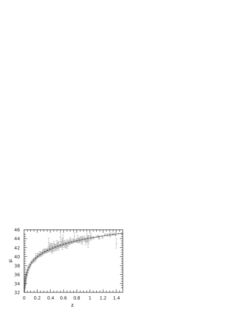
Figure 2: Best-fit for the distance modulus versus redshift for the Visser model (solid gray line) and the $\Lambda$CDM model (dashed line). The SNe data were taken from the Union2 compilation Amanullah and et al. (2010).

IV.4 Joint analysis

When the measurements of SNe Ia luminosity distances are combined with information related to the Baryon Acoustic Oscillation (BAO) peak and the CMB shift parameter, the constraining power of the fit to the parameters in the cosmological model is greatly improved. Following such an approach we examine here the effects of summing up the contributions of these last two parameters into the $\chi^{2}$ of Eq. (14). Our result is $\Omega_{m}=0.273\pm 0.015$ with the corresponding minimum value for the $\chi^{2}$ function: $\chi^{2}_{min}=565.06$.

We can compare our results with the $\Lambda$CDM model by taking the difference between $\chi^{2}_{g}$ and $\chi^{2}_{\Lambda CDM}$, which are the minimum $\chi^{2}$ values for the massive bimetric model and for the $\Lambda$CDM model, respectively. The evaluation of this difference gives the result $\Delta\chi^{2}=\chi^{2}_{g}-\chi^{2}_{\Lambda CDM}=21.30$, which shows that the bimetric Visser’s model is disfavored when compared with the flat $\Lambda$CDM model.

In the Table 1 we summarize our results for $\Omega_{m}$ considering each cosmological observable: SNe, CMB, BAO and the combined analysis (SNe+CMB+BAO). For the sake of comparison it is also shown the values of $\chi^{2}_{min}$ and $\Omega_{m}$ for the $\Lambda$CDM model.

It is also instructive to evaluate the effect of adding the systematic uncertainties of the SNe analysis on our results. Considering only SNe, the addition of the systematic erros to the statistical erros lead us to $\Omega_{m}=0.295^{+0.039}_{-0.036}$ for the Visser’s model. We also obtain a considerable lower value for the difference between the $\chi^{2}$ of the two models $\Delta\chi^{2}=8.11$. Now, taking into account the CMB and BAO measurements together with SNe, we obtain $\Omega_{m}=0.290^{+0.020}_{-0.019}$ and $\Delta\chi^{2}=10.26$ (see Table 1).

In the Fig. 1 and Fig. 2 we show the Hubble parameter and the distance modulus as functions of redshift considering the best-fit value of $\Omega_{m}$ for the SNe. For the sake of comparison, the standard $\Lambda$CDM model is also shown. Note that although the massive graviton model is disfavored, it seems to be able to reproduce very well the SNe Ia measurements, as can be seen in the Fig. 2. This shows the importance of the $\chi^{2}$ test in distinguishing the two models.

IV.5 Effective equation of state

The Fig. (3) shows the effective equation of state

$$w_{eff}(z)=-1+\frac{2(1+z)}{3H}\frac{dH}{dz}$$ (19)

as a function of the redshift for the best-fit values above. The deceleration parameter, which is shown in the Fig.4, is related to $w_{eff}$ through $q(z)=(3w_{eff}(z)+1)/2$. In order to plot these curves we have included a component of radiation with the present value of the density parameter $\Omega_{r}=5\times 10^{-5}$. For the best-fit value found in our analysis, the Visser model goes through the last three phases of cosmological evolution, i.e., radiation-dominated $(w=1/3)$, matter-dominated $(w=0)$ and the late time acceleration phase $(w<-1/3)$.

Note that for low redshifts the Visser’s model shows additionally a phase dominated by matter, indicating that for this model the late time acceleration of the Universe was a transient phase which has already finished. Moreover, for low redshifts, this behavior of the Visser’s theory is in accordance with the fact that the luminosity distance of very low redshift SNe Ia can be fitted with CDM model only, i.e., at very low redshift the $\Lambda$CDM, CDM and Visser’s model are degenerate for the cosmological observations.

Figure 3: Effective state parameter as a function of the redshift for the best-fit value obtained from SNe Ia.

Figure 4: Deceleration parameter as a function of the redshift for the best-fit value obtained from SNe Ia. Note that the acceleration phase is transient in the Visser model.

V Conclusions

The theory of massive gravitons as considered in the Visser’s approach has the advantage that the field equations (3) differs from Einstein equations only in a subtle way, namely, by the introduction of the bimetric mass tensor $M_{\mu\nu}$. Moreover the van Dam-Veltmann-Zakharov discontinuity (vDVZ) present in the Pauli-Fierz term can be circumvented in Visser’s model by introducing a non-dynamical flat-background metric Will .

From the cosmological point of view, the meaning of the mass tensor, classically speaking, is a long range correction to the ordinary Friedmann equation. Such a correction mimics the effects of a dark energy component in such a way that additional fields are not necessary.

In this context, we have shown that the cosmological model with massive gravitons could be a viable explanation to the dark energy problem. But, although the parameter $\Omega_{m}$ is well constrained, the model is disfavored when compared to the $\Lambda$CDM model. Considering systematic errors, the difference between the $\chi^{2}_{min}$ of the two models reduces considerably, but the the Visser model is still disfavored.

Finally, the plots of the effective state parameter and of the deceleration parameter for the best fit value of $\Omega_{m}$, show a very particular feature of the Visser’s model, namely, the transient behavior of the accelerated phase of expansion. The Universe begins to accelerate approximately at the same redshift of the $\Lambda$CDM model, but for a very small redshift ($z\sim 4\times 10^{-2}$) we have a second transition and the Universe becomes to decelerate again. In spite of this, the behavior of the Hubble parameter $H(z)$ is very similar in both models as can be seen in the Fig.1. In this way, one would think that the transient acceleration phase is what make the Visser model less compatible with SNe data than the $\Lambda$CDM model. This is a problem which we will address in the future in order to find consistent modifications of Visser’s approach.

References

- Spergel and et al. (2007) D. N. Spergel and et al. (2007), eprint astro-ph/0603449.
- Perlmutter et al. (1999) S. Perlmutter et al. (Supernova Cosmology Project), Astrophys. J. 517, 565 (1999), eprint astro-ph/9812133.
- Riess et al. (1998) A. G. Riess et al. (Supernova Search Team), Astron. J. 116, 1009 (1998), eprint astro-ph/9805201.
- Riess et al. (2007) A. G. Riess et al., Astrophys. J. 659, 98 (2007), eprint astro-ph/0611572.
- Komatsu et al. (2008) E. Komatsu et al. (WMAP) (2008), eprint 0803.0547.
- Tegmark et al. (2004) M. Tegmark et al. (SDSS), Phys. Rev. D69, 103501 (2004), eprint astro-ph/0310723.
- Cole et al. (2005) S. Cole et al. (The 2dFGRS), Mon. Not. Roy. Astron. Soc. 362, 505 (2005), eprint astro-ph/0501174.
- Carroll et al. (2004) S. M. Carroll, V. Duvvuri, M. Trodden, and M. S. Turner, Phys. Rev. D70, 043528 (2004), eprint astro-ph/0306438.
- Nojiri and Odintsov (2004) S. Nojiri and S. D. Odintsov, Gen. Rel. Grav. 36, 1765 (2004), eprint hep-th/0308176.
- Santos et al. (2008) J. Santos, J. S. Alcaniz, F. C. Carvalho, and N. Pires, Phys. Lett. B669, 14 (2008), eprint 0808.4152.
- Carvalho et al. (2008) F. C. Carvalho, E. M. Santos, J. S. Alcaniz, and J. Santos, JCAP 0809, 008 (2008), eprint 0804.2878.
- Santos et al. (2007) J. Santos, J. S. Alcaniz, M. J. Reboucas, and F. C. Carvalho, Phys. Rev. D76, 083513 (2007), eprint 0708.0411.
- Alves et al. (2009a) M. E. S. Alves, O. D. Miranda, and J. C. N. de Araujo, Phys. Lett. B 679, 401 (2009a).
- Visser (1998) M. Visser, General Relativity and Gravitation 30, 1717 (1998).
- Talmadge et al. (1988) C. Talmadge, J. P. Berthias, R. W. Hellings, and E. M. Standish, Phys. Rev. Lett. 61, 1159 (1988).
- Goldhaber and Nieto (1974) A. S. Goldhaber and M. M. Nieto, Phys. Rev. D 9, 1119 (1974).
- de Araujo and Miranda (2007) J. C. N. de Araujo and O. D. Miranda, Gen. Relativ. and Gravit. 39, 777 (2007).
- Finn and Sutton (2002) L. S. Finn and P. J. Sutton, Phys. Rev. D 65, 044022 (2002).
- Bessada and Miranda (2009a) D. Bessada and O. D. Miranda, JCAP 08, 33 (2009a).
- Bessada and Miranda (2009b) D. Bessada and O. D. Miranda, Class. Quantum Grav. 26, 045005 (2009b).
- de Paula et al. (2004) W. L. S. de Paula, O. D. Miranda, and R. M. Marinho, Class. Quantum Grav. 21, 4595 (2004).
- Amanullah and et al. (2010) R. Amanullah and et al. (2010), eprint astro-ph/0603449.
- Eisenstein et al. (2005) D. J. Eisenstein et al. (SDSS), Astrophys. J. 633, 560 (2005), eprint astro-ph/0501171.
- Spergel et al. (2007) D. N. Spergel et al. (WMAP), Astrophys. J. Suppl. 170, 377 (2007), eprint astro-ph/0603449.
- Narlikar (1984) J. Narlikar, J. Astrophys. Astr. 5, 67 (1984).
- Rastall (1972) P. Rastall, Phys. Rev. D 6, 3357 (1972).
- Alves et al. (2007) M. E. S. Alves, O. D. Miranda, and J. C. N. de Araujo, Gen. Relativ. and Gravit. 39, 777 (2007).
- Alves et al. (2009b) M. E. S. Alves, O. D. Miranda, and J. C. N. de Araujo (2009b), eprint astro-ph/0907.5190.
- Bond et al. (1997) J. R. Bond, G. Efstathiou, and M. Tegmark, Mon. Not. Roy. Astron. Soc. 291, L33 (1997), eprint astro-ph/9702100.
- (30) C. M. Will, eprint Living Reviews in Relativity - http://relativity.livingreviews.org/Articles/Irr-2006-3.