The three-site Bose-Hubbard model subject to atom losses: the boson-pair dissipation channel and failure of the mean-field approach

Abstract

We employ the perturbation series expansion for derivation of the reduced master equations for the three-site Bose-Hubbard model subject to strong atom losses from the central site. The model describes a condensate trapped in a triple-well potential subject to externally controlled removal of atoms. We find that the $\pi$-phase state of the coherent superposition between the side wells decays via two dissipation channels, the single-boson channel (similar to the externally applied dissipation) and the boson-pair channel. The quantum derivation is compared to the classical adiabatic elimination within the mean-field approximation. We find that the boson-pair dissipation channel is not captured by the mean-field model, whereas the single-boson channel is described by it. Moreover, there is a matching condition between the zero-point energy bias of the side wells and the nonlinear interaction parameter which separates the regions where either the single-boson or the boson-pair dissipation channel dominate. Our results indicate that the $M$-site Bose-Hubbard models, for $M>2$, subject to atom losses may require an analysis which goes beyond the usual mean-field approximation for correct description of their dissipative features. This is an important result in view of the recent experimental works on the single site addressability of condensates trapped in optical lattices.

I Introduction

The mean-field approximation, formally obtained by replacing the boson creation and annihilation operators by complex scalars, is usually employed for description of bosonic many-body systems when the number of bosons is large (for instance, see Refs. BStat ; CD ; GP ). Such a replacement can be justified by the $\sqrt{N}$-scaling of the boson operators, that is, when the populations are large, the commutators – the source of quantum corrections – are negligible BStat . The relation between the quantum and mean-field descriptions is a subject of intensive studies. The quantum description is necessary for the bifurcations, which modify significantly the quantum spectrum AFKO , the quantum collapses and revivals MCWW , and the many-body quantum corrections to the mean-field theory VA ; AV . Making explicit the $N$-scaling of the operators and identifying the $N$-scaling of the parameters for a fixed particle density, reveals the link of the mean-field approximation to the Wentzel-Kramers-Brillouin semiclassical approach to the discrete Schrödinger equation Braun , now employed in the Fock space with the inverse number of bosons $1/N$ playing the role of an effective Planck constant (see, for example, Ref. ST ). Therefore, the mean-field limit, as the semiclassical limit of a discrete Schrödinger equation, is also singular. Hence, besides the pronounced quantum corrections/fluctuations at the bifurcations/instabilities, one must be prepared to find even a qualitative disagreement between the mean-field description and the full quantum consideration even when the populations are large, as it is the case, for instance, in the nonlinear boson model which describes tunneling of boson pairs between two modes, see Refs. SK ; MsQ .

The main purpose of the present paper is to study the dissipation dynamics of the atom filled lattice sites coupled to a common dissipated sites. Our motivation is the recent advancement in the quantum microscopy techniques and the current experiments on the single site addressability in the optical lattices SiteAddr1 ; SiteAddr2 , where controlled atom losses are induced in selected sites of a two-dimensional optical lattice. We develop a direct method based on the perturbation expansion for derivation of the reduced quantum master equations for the Bose-Hubbard models with dissipation (we consider the atom losses) and compare the quantum derivation with the mean-field description. We concentrate on the three-site Bose-Hubbard model, which is the simplest model describing atom filled sites coupled to a common dissipated one and describes, for instance, cold atoms or Bose-Einstein condensate trapped in a triple-well potential subject to removal of atoms from the central well, see Fig. 1. The three-site Bose-Hubbard model was also noted to possess many features of complexity of a general quantum dynamics, as the Wigner-Dyson spectral statistics and quantum chaos WDSt ; Chaos3w . It is also the simplest model where the boson-pair tunneling, originating from the nonlinearity of the model, is possible.

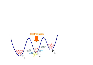
Figure 1: (Color online) The three-site Bose-Hubbard model setup. A laser/electron beam removes atoms from the central well with a rate $\Gamma$. The $\varepsilon_{j}$ represents the zero-point energy of the $j$th well. The two quantum channels of dissipation of the $\pi$-phase coherent mode, described in the text, are shown schematically by arrows.

We derive the reduced quantum master equations for the coherent modes describing the condensate in the side wells, then consider the mean-field approach and compare the results of the two approaches. We note here that we consider an open quantum system and, as such, described by the quantum master equation CBook ; BP . However, in the case of the atom losses, the mean-field formulation is straightforward (this also applies to the case of the multiple-site atom losses of the experimental works of Refs. SiteAddr1 ; SiteAddr2 ). Contrary to the fact that the mean-field approximation applies with a good accuracy to the two-site Bose-Hubbard model with atoms losses and a noise TWW ; NlZeno , it is shown here that the correct and complete description of the three-site model (in general, the $M$-site Bose-Hubbard models, with $M\geq 3$) requires going beyond the usual mean-field approach. This disagreement stems from the quantum boson-pair dissipation channel, due to the nonlinear interaction (this is similar to the boson-pair tunneling resulting in the qualitative failure of the mean-field approach in Ref. MsQ ). Moreover, there is a matching condition between the zero-point energy bias of the side wells and the nonlinear interaction parameter which separates the regions where either the single-boson or the boson-pair dissipation channel dominate. Hence, one has to use the full quantum consideration, i.e. the quantum master equation reduction methods, to describe the decay of the subsystem (in our case, the quantum modes describing the side wells), which then may be treated with further approximations, even resembling the mean-field approach. However, the point is that without invoking the quantum consideration at some stage, i.e. working just within the mean-field approach, one will be unable to describe the dissipative behavior of the filled sites coupled to a common dissipated site, which conclusion is also relevant to the recent experiments of Ref. SiteAddr1 .

The paper is organized as follows. In section II we formulate the quantum master equation. The derivation of the reduced master equation for the side modes (i.e., the coherent superposition modes over the left and right wells in Fig. 1) is given in section III. In section IV a similar reduction is applied to the reduced master equation of section III producing the master equation for the $\pi$-phase coherent mode. In section V the adiabatic elimination within the mean-field approximation is studied. The concluding remarks and discussion is contained in section VI.

II The problem formulation in terms of the master equation

A quantum channel representation for a local atom losses (e.g., from a single lattice site), see Fig. 1, can be given in the Fock space as follows NlZeno

$$|k_{j}\rangle|0\rangle_{R}\to\sqrt{p}|k_{j}-1\rangle|1\rangle_{R}+\sqrt{1-p}|k_{j}\rangle|0\rangle_{R},$$

$|k_{j}\rangle$ is the ket-vector of the Fock space of a dissipating boson mode, $|X\rangle_{R}$ describes the atom counter, and $p=p(k_{j},t)$ is the probability. Note that $p(k_{j},\delta t)$, for small $\delta t$, depends linearly on the number of atoms in the dissipating mode. As the result, a Lindblad term with the generator $L=\sqrt{\Gamma}a_{j}$ appears in the master equation for the density matrix. Here $\Gamma$ is the dissipation rate parameter. We consider the dissipation acting on the central well (denoted with $j=3$ in Fig. 1) of the triple-well trap, thus the master equation for the density matrix reads

$$\frac{d\rho}{dt}=-\frac{i}{\hbar}[H,\rho]+\Gamma\left(a_{3}\rho a^{\dagger}_{3}-\frac{1}{2}n_{3}\rho-\frac{1}{2}\rho n_{3}\right).$$ (1)

By $H$ we denote the three-site Bose-Hubbard Hamiltonian,

$$H=-J([a_{1}^{\dagger}+a_{2}^{\dagger}]a_{3}+a_{3}^{\dagger}[a_{1}+a_{2}])+\sum_{j=1}^{3}\varepsilon_{j}a^{\dagger}_{j}a_{j}+U\sum_{j=1}^{3}(a^{\dagger}_{j})^{2}a_{j}^{2},$$ (2)

where $a_{j}$ and $a_{j}^{\dagger}$ ($j=1,2,3$) are the local boson modes describing occupation of the respective well, $J$ is the linear tunneling rate, $\varepsilon_{j}$ is the zero-point energy of the respective well, and $U$ is the atomic interaction parameter proportional to the $s$-wave scattering length.

Due to the linear coupling of the central well to the side wells in the Bose-Hubbard model, it is convenient to use the new canonical basis $b_{1}=(a_{1}+a_{2})/{\sqrt{2}}$, $b_{2}=(a_{1}-a_{2})/{\sqrt{2}}$, and $b_{3}=a_{3}$. Here the modes $b_{1,2}$ describe, respectively, the zero-phase and $\pi$-phase coherent superpositions between the side wells. The Bose-Hubbard Hamiltonian becomes

$$H = -J_{13}(b^{\dagger}_{1}b_{3}+b^{\dagger}_{3}b_{1})-J_{12}(b^{\dagger}_{1}b_{2}+b^{\dagger}_{2}b_{1})+\varepsilon n_{3}$$ (3)

$$+ Un_{3}^{2}+\frac{U}{2}\left([n_{1}+n_{2}]^{2}+[b^{\dagger}_{1}b_{2}+b^{\dagger}_{2}b_{1}]^{2}\right),$$

where $n_{j}=b^{\dagger}_{j}b_{j}$ and we have introduced the parameters $J_{13}=\sqrt{2}J$, $J_{12}=(\varepsilon_{2}-\varepsilon_{1})/2$, $\varepsilon=\varepsilon_{3}-(\varepsilon_{1}+\varepsilon_{2})/2$ (and dropped an inessential term proportional to $N=n_{1}+n_{2}+n_{3}$).

III The reduced master equation for the side wells

In the strongly dissipative case, $\Gamma\gg J_{13}/\hbar$, the central well is emptied on the time scale $t\sim 1/\Gamma$, while the coherent modes $b_{1}$ and $b_{2}$ almost retain their populations (see also Ref. NlZeno ). It turns out that in this case one can derive an approximate master equation for the side wells alone valid for the times $t\gg 1/\Gamma$, when the central-well dissipation has the fastest time-scale in the system. Introducing the small parameter $\epsilon=J_{13}/\hbar\Gamma$ we require that $J_{12}/\hbar\Gamma=\mathcal{O}(\epsilon)$ and $U\langle n_{1,2}\rangle/\hbar\Gamma=\mathcal{O}(\epsilon)$. This approximation is valid for an arbitrary bias $\varepsilon$ between the central and side wells. We will see that, already in the first order in $\epsilon$, the density matrix for the whole system is not factorized and the central-well population strongly depends on that of the side wells. Nevertheless, in the higher orders of the perturbation theory (namely, in the second and third orders in $\epsilon$), the central well acts as an effective reservoir for the side wells leading to the master equation in the standard Lindblad form.

First of all, let us pass to the interaction picture. Introduce

$$\hat{H}_{I}(t)=U_{0}^{\dagger}(t)H_{I}U_{0}(t),\quad\hat{\rho}=U_{0}^{\dagger}(t)\rho(t)U_{0}(t)$$

$$U_{0}(t)=U_{12}(t)\otimes U_{3}(t)=\exp\{-\frac{i}{\hbar}(H_{12}\!+\!H_{3})\Delta t\},$$ (4)

where $\Delta t=t-t_{0}$, $t_{0}$ is some initial time, and $H_{12}$, $H_{3}$ and $H_{I}$ are parts of the Hamiltonian (3) describing the side wells, the central well and the interaction between them, respectively (we have also subtracted the nonessential term $U(n_{1}+n_{2}+n_{3})$ from the system Hamiltonian to simplify the presentation). The master equation in the interaction picture reads

$$\frac{d\hat{\rho}}{dt}=-\frac{i}{\hbar}[\hat{H}_{I}(t),\hat{\rho}]+\Gamma\left(\hat{b}_{3}(t)\hat{\rho}\hat{b}^{\dagger}_{3}(t)-\frac{1}{2}\hat{n}_{3}\hat{\rho}-\frac{1}{2}\hat{\rho}\hat{n}_{3}\right),$$ (5)

where $\hat{b}_{3}(t)=U_{0}^{\dagger}(t)b_{3}U_{0}(t)$. Below we will work in the interaction picture and drop the hat, for simplicity. The density matrix expansion reads $\rho=\rho^{(0)}_{12}\otimes\rho^{(0)}_{3}+\rho^{(1)}+\rho^{(2)}+\mathcal{O}(\epsilon^{3})$, where, for instance, $\rho_{12}=\mathrm{Tr}_{3}\{\rho\}$ (an arbitrary non-factorized expansion, $\rho^{(0)}=\sum_{ij}c_{ij}\rho^{(0)}_{12i}\otimes\rho^{(0)}_{3j}$, leads to the same result). In the lowest orders in $\epsilon$ we have:

$$\frac{d\rho^{(0)}_{12}}{dt}=0,\quad\frac{d\rho^{(0)}_{3}}{dt}=\Gamma D(t)\{\rho_{3}^{(0)}\},$$ (6)

$$\frac{d\rho^{(1)}}{dt}=-\frac{i}{\hbar}[H_{I}(t),\rho^{(0)}_{12}\otimes\rho^{(0)}_{3}]+\Gamma D(t)\{\rho^{(1)}\},$$ (7)

$$\frac{d\rho^{(2)}_{12}}{dt}=-\frac{i}{\hbar}\mathrm{Tr}_{3}\{[H_{I}(t),\rho^{(1)}]\}.$$ (8)

The solution to the equation for $\rho^{(0)}_{3}$ is as follows

$$\rho^{(0)}_{3}(t)=|0\rangle\langle 0|+e^{-\frac{\Gamma}{2}\Delta t}\left[c_{1}|1\rangle\langle 0|+h.c.\right]+\mathcal{O}(e^{-\Gamma\Delta t}),$$ (9)

where the last term represents all higher-order external products of the Fock basis states and a decaying renormalization correction to the first term. The coefficient $c_{1}$ has the following meaning: $\mathrm{Tr}_{3}\{b_{3}(t)\rho_{3}^{(0)}(t)\}=c_{1}f_{1}(t)e^{-\frac{\Gamma}{2}\Delta t}+\mathcal{O}(e^{-\Gamma\Delta t})$, with $f_{1}$ being the eigenvalue of the unitary transformation in Eq. (5): $U_{3}(t)|1\rangle=f_{1}(t)|1\rangle$, in our case $f_{1}(t)=e^{-i\varepsilon\Delta t/\hbar}$ (note also that $b_{3}(t)=f_{1}(t)b_{3}$).

Inserting Eq. (9) into Eq. (7) we get the general solution in the following form (suggested by the form of $\rho^{(0)}_{3}$ itself)

$$\rho^{(1)}(t)=V(t)\left[\rho^{(0+1)}_{12}\otimes|0\rangle\langle 0|\right]V^{\dagger}(t)+\mathcal{O}(e^{-\frac{\Gamma}{2}\Delta t}),$$ (10)

where $\rho^{(0+1)}_{12}=\rho^{(0)}_{12}+\rho^{(1)}_{12}$ and $V(t)$ reads

$$V(t)=\exp\{\alpha_{1}(t)b_{1}(t)b^{\dagger}_{3}(t)\}=I+\alpha_{1}(t)b_{1}(t)b^{\dagger}_{3}(t)+\mathcal{O}(\epsilon^{2}),$$ (11)

with a scalar function $\alpha_{1}(t)=\mathcal{O}(\epsilon)$. Indeed, taking derivative of the solution (11) and using Eqs. (7) and (9), we obtain the equation to be satisfied

$$\frac{d\rho^{(1)}}{dt}=\frac{dV}{dt}\rho^{(0)}_{12}\otimes|0\rangle\langle 0|V^{\dagger}+V\rho^{(0)}_{12}\otimes|0\rangle\langle 0|\frac{dV^{\dagger}}{dt}$$

$$+V\frac{d\rho^{(1)}_{12}}{dt}\otimes|0\rangle\langle 0|V^{\dagger}=-\frac{i}{\hbar}[H_{I}(t),\rho^{(0)}_{12}\otimes|0\rangle\langle 0|]$$

$$+\Gamma D\{V\rho^{(0+1)}_{12}\otimes|0\rangle\langle 0|V^{\dagger}\}+\mathcal{O}(\epsilon^{2}).$$ (12)

We evaluate

$$-\frac{i}{\hbar}[H_{I}(t),\rho^{(0)}_{12}\otimes|0\rangle\langle 0|]\qquad\qquad$$

$$=\frac{iJ_{13}}{\hbar}\bigl{(}f^{*}_{1}(t)b_{1}(t)\rho^{(0)}_{12}\otimes|1\rangle\langle 0|-h.c.\bigr{)}$$ (13)

and, using Eq. (11),

$$\Gamma D(t)\{V\rho^{(0+1)}_{12}\otimes|0\rangle\langle 0|V^{\dagger}\}\qquad\qquad$$

$$=-\frac{\Gamma}{2}\left(\alpha_{1}(t)f^{*}_{1}(t)b_{1}(t)\rho^{(0)}_{12}\otimes|1\rangle\langle 0|+h.c.\right)+\mathcal{O}(\epsilon^{2}).\qquad$$ (14)

Eqs. (7) and (13) give immediately

$$\frac{d{\rho}^{(1)}_{12}}{dt}=\mathcal{O}(e^{-\frac{\Gamma}{2}\Delta t}).$$ (15)

Since $J_{12}/\hbar\Gamma=\mathcal{O}(\epsilon)$ and $U\langle n_{1,2}\rangle/\hbar\Gamma=\mathcal{O}(\epsilon)$, the derivative of $b_{1}(t)$ is of order $\epsilon$,

$$\frac{db_{1}(t)}{dt}=-\frac{i}{\hbar}[H_{12},b_{1}(t)]=\mathcal{O}(\epsilon).$$ (16)

Now, by taking into account Eqs. (11), (13)-(16), one sees that Eq. (12) is satisfied by setting

$$\frac{d\alpha_{1}}{dt}=-\left[\frac{\Gamma}{2}+i\frac{\varepsilon}{\hbar}\right]\alpha_{1}+\frac{iJ_{13}}{\hbar}.$$ (17)

Equation (17) gives

$$\alpha_{1}=\frac{2iJ_{13}}{\hbar\Gamma}\left[1+\frac{2i\varepsilon}{\hbar\Gamma}\right]^{-1}+\mathcal{O}(e^{-\frac{\Gamma}{2}\Delta t}).$$ (18)

The final step is to insert Eq. (10) into Eq. (8), use Eqs. (6) and (15) and take the trace over the central-well subspace, keeping only the terms up to $\mathcal{O}(\epsilon^{2})$. Returning to the Schrödinger picture, we get (up to a correction of the order $\mathcal{O}(\epsilon^{3})$)

$$\frac{d{\rho}_{12}}{dt} = -\frac{i}{\hbar}[H_{12},{\rho}_{12}]-\frac{i}{\hbar}[\varepsilon_{R}b^{\dagger}_{1}b_{1},{\rho}^{(0)}_{12}]+\Gamma_{R}D_{1}\{{\rho}^{(0)}_{12}\}$$ (19)

$$+\mathcal{O}(e^{-\frac{\Gamma}{2}\Delta t}),$$

with $\Gamma_{R}$ given by

$$\Gamma_{R}=|\alpha_{1}|^{2}\Gamma=\frac{4J_{13}^{2}}{\hbar^{2}\Gamma}\left[1+\left(\frac{2\varepsilon}{\hbar\Gamma}\right)^{2}\right]^{-1},$$ (20)

and $D_{1}\{{\rho}\}=b_{1}{\rho}b^{\dagger}_{1}-\frac{1}{2}\{b^{\dagger}_{1}b_{1},{\rho}\}$. The interaction-induced Lamb shift $\varepsilon_{R}$ of the zero-point energy of the coherent zero-phase mode $b_{1}$ reads

$$\varepsilon_{R}=-J_{13}\mathrm{Re}(\alpha_{1})=-\varepsilon\frac{\Gamma_{R}}{\Gamma}.$$ (21)

Our aim is to further reduce Eq. (19) to a master equation for the coherent $\pi$-phase mode $b_{2}$, which has unusual dissipation features (see below). To this end, however, one has to consider the contribution to Eq. (19) coming from the next order in $\epsilon$, i.e. $\mathcal{O}(\epsilon^{3})$. Indeed, similar to the derivation of this section, the reduced master equation for mode $b_{2}$ is obtained under the conditions that $J_{12},U\langle n_{1,2}\rangle\ll\hbar\Gamma_{R}$, what makes the Hamiltonian part in the master equation (19) smaller than the Lindblad part, hence the former should be discarded in the present order $\mathcal{O}(\epsilon^{2})$. Thus, in the second-order approximation, the coherent mode $b_{2}$ has no dissipation dynamics at all (only the Hamiltonian evolution described by $H_{2}=\frac{U}{2}n_{2}^{2}$). It only appears in the higher-order version of the master equation (19).

To derive the third-order correction to Eq. (19), we need to find the form of $\rho^{(2)}(t)$, which satisfies equation similar to Eq. (7), but now with the inhomogeneous term

$$-\frac{i}{\hbar}[H_{I}(t),V\rho^{(0+1)}_{12}\otimes|0\rangle\langle 0|V^{\dagger}]$$

$$=\frac{iJ_{13}}{\hbar}\biggl{\{}\left(\sqrt{2}\alpha_{1}(t)f_{2}^{*}(t)b_{1}^{2}(t)\rho_{12}^{(0)}\otimes|2\rangle\langle 0|-h.c.\right)$$

$$-2i\mathrm{Im}\{\alpha_{1}(t)\}b_{1}(t)\rho_{12}^{(0)}b_{1}^{\dagger}(t)\otimes|1\rangle\langle 1|$$

$$+\left(\alpha_{1}(t)b_{1}^{\dagger}(t)b_{1}(t)\rho^{(0)}_{12}-h.c.\right)\otimes|0\rangle\langle 0|$$

$$+\left(f_{1}^{*}(t)b_{1}(t)\rho_{12}^{(1)}\otimes|1\rangle\langle 0|-h.c.\right)\biggr{\}}+\mathcal{O}(\epsilon^{2}),$$ (22)

where $U_{3}(t)|2\rangle=f_{2}(t)|2\rangle$, i.e. $f_{2}=e^{-2i\frac{(\varepsilon+U)}{\hbar}\Delta t}$. The first three lines of Eq. (22) give the terms additional to those in Eq. (13). Expression (22) also defines the general form of $\rho^{(2)}(t)$:

$$\rho^{(2)}=B_{00}(t)\otimes|0\rangle\langle 0|+B_{11}(t)\otimes|1\rangle\langle 1|$$

$$+\left(B_{10}(t)\otimes|1\rangle\langle 0|+B_{20}(t)\otimes|2\rangle\langle 0|+h.c.\right),$$ (23)

where the operators $B_{ij}(t)=\mathcal{O}(\epsilon^{2})$ act on the subspace of the side wells. They satisfy, in view of Eqs. (20), (13), (15), (21) and (22), the following equations:

$$\frac{dB_{11}}{dt} = -\Gamma B_{11}+\Gamma_{R}b_{1}(t)\rho_{12}^{(0)}b_{1}^{\dagger}(t),$$ (24a)

$$\frac{dB_{00}}{dt} = \Gamma B_{11}-\frac{i}{\hbar}[\varepsilon_{R}n_{1}(t),\rho_{12}^{(0)}]$$ (24b)

$$-\frac{\Gamma_{R}}{2}\left(n_{1}(t)\rho_{12}^{(0)}+\rho_{12}^{(0)}n_{1}(t)\right),$$

$$B_{10} = \alpha_{1}(t)f_{1}^{*}(t)b_{1}(t)\rho_{12}^{(1)},$$ (24c)

$$B_{20} = \alpha_{2}(t)f^{*}_{2}(t)b_{1}^{2}(t)\rho_{12}^{(0)},$$ (24d)

where $\alpha_{1}(t)$ is given by Eq. (18) and

$$\frac{d\alpha_{2}}{dt}=-\left[\frac{\Gamma}{2}+i\frac{\varepsilon+U}{\hbar}\right]\alpha_{2}+i\frac{\sqrt{2}J_{13}}{\hbar}\alpha_{1}(t).$$ (25)

One can easily solve Eq. (24a) and by using integration by parts represent the result as

$$B_{11}(t)=\frac{\Gamma_{R}}{\Gamma}b_{1}(t)\rho^{(0)}_{12}b_{1}^{\dagger}(t)+\mathcal{O}(\epsilon^{3})+\mathcal{O}(e^{-\Gamma\Delta t}).$$ (26)

Substituting Eq. (26) into Eq. (24b) and using the master equation (19) one obtains

$$B_{00}(t)=\rho_{12}^{(2)}+\mathcal{O}(e^{-\Gamma\Delta t}).$$ (27)

Finally, the solution to Eq. (25) reads

$$\alpha_{2}(t) = -\frac{2\sqrt{2}J^{2}_{13}}{\hbar^{2}\Gamma^{2}}\left[1+i\frac{2\varepsilon}{\hbar\Gamma}\right]^{-1}\left[1+i\frac{2(\varepsilon+U)}{\hbar\Gamma}\right]^{-1}$$ (28)

$$+ \mathcal{O}(e^{-\frac{\Gamma}{2}\Delta t})=\frac{\alpha_{1}^{2}(t)}{\sqrt{2}}+\mathcal{O}(\epsilon^{3})+\mathcal{O}(e^{-\frac{\Gamma}{2}\Delta t}).$$

The fact that the operators $B_{11}$ and $B_{20}$ and $B_{02}$ do not contribute to the equation for $\rho_{12}$ and the explicit expressions for $B_{00}$ and $B_{10}$, Eqs. (26) and (27), lead to the same Lindblad form of the reduced master equation, i.e. in the Schrödinger picture we get

$$\frac{d\rho_{12}}{dt}=-\frac{i}{\hbar}[H_{12}+\varepsilon_{R}n_{1},\rho_{12}]+\Gamma_{R}D_{1}\{\rho_{12}\}+\mathcal{O}(e^{-\frac{\Gamma}{2}\Delta t}),$$ (29)

which is now valid up to correction of order $\mathcal{O}(\epsilon^{4})$. Eqs. (23), (26)-(28) also show that the density matrix of the full system $\rho$ can be rewritten as (now in the Schrödinger picture)

$$\rho(t)=V\left[\rho_{12}(t)\otimes|0\rangle\langle 0|\right]V^{\dagger}+\mathcal{O}(\epsilon^{3})+\mathcal{O}(e^{-\frac{\Gamma}{2}\Delta t}),$$ (30)

where $\rho_{12}(t)$ is taken up to the second order in $\epsilon$, $V(t)=\exp\{\alpha_{1}b_{1}b^{\dagger}_{3}\}=I+\alpha_{1}b_{1}b^{\dagger}_{3}+\frac{1}{2}\alpha_{1}^{2}b^{2}_{1}(b^{\dagger}_{3})^{2}$ with $\alpha_{1}$ given by Eq. (18). Eqs. (29) and (30) are the main results of this section. Obviously, the full density matrix (30) is not factorized, nevertheless, the reduced density matrix of a subsystem satisfies the Markovian master equation (29) in the Lindblad form. Note that the difference between the density matrix $\rho_{12}$ and the one obtained by tracing the full density matrix of Eq. (30) is a constant term of the second order given by $B_{11}$ in Eq. (26), which does not contribute to Eq. (29). Hence, Eq. (30) is consistent with the approximation made.

In Fig. 2, we use the Monte Carlo wave-function method MCD and find that an excellent agreement of the reduced master equation (29) with the full Eq. (1) extends also to the intermediate values of $\Gamma$ (we have there $\epsilon=0.2$). We have also verified that, for large $\Gamma$, the modes $a_{1,2}$ (and, hence, $b_{1,2}$) stay practically unchanged while the dissipating mode $b_{3}=a_{3}$ is quickly emptied (the inset of Fig. 2).

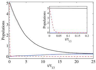
Figure 2: (Color online) Comparison between the full 3-mode Eq. (1) and the reduced 2-mode Eq. (29). The population of $a_{3}$ is given by the dashed lines. The populations of modes $a_{1}$ and $a_{2}$ (solid lines) of the 3-mode model are compared to that of the 2-mode model (dotted lines). Here $\Gamma=5J/\hbar$, $U=0.2J$, $\varepsilon_{j}=0$. We have used 5000 quantum trajectories. The inset shows the short-time dynamics of populations for larger $\Gamma=50J/\hbar$. The initial state is the Fock state with the total of 10 atoms (5 occupying the mode $a_{1}$ and 5 occupying the mode $a_{3}$.

Let us note the specific features of Eq. (29). We see that in the strongly dissipative case, quite similar to Eq. (1), mode $b_{2}$ can retain a significant part of its population, while $b_{1}$ loses almost all atoms, on the time scale $t\sim 1/\Gamma_{R}$, and after that stays practically empty. In the long run, on the time scale much longer that $1/\Gamma_{R}$, the population of mode $b_{2}$ drops to the single-atom level (this is seen also in Fig. 2, where it happens on the short time scale due to a small $\Gamma$).

In the linear case Eq. (29) acts like a dispersive beam-splitter (see, for example, Ref. mogilevtsev2009 ). Thus, a strong loss in the central well induces quantum correlations between the side wells, i.e. for times $t\gg 1/\Gamma_{R}$ the cold atoms occupy the state

$$|\Psi_{n}\rangle\sim(b_{2}^{\dagger})^{n}|0\rangle\sim(a_{1}^{\dagger}-a_{2}^{\dagger})^{n}|0\rangle$$ (31)

which is unaffected by the dissipation described by Eq. (29).

In the nonlinear case, the dissipation of the $\pi$-phase mode $b_{2}$ is surprisingly non-trivial. This can be clearly demonstrated in the case when the decay of the zero-phase mode $b_{1}$ occurs on the faster scale than the inter-mode dynamics. To uncover the details, let us use the higher-order validity of Eq. (29) and reduce it to a single-mode master equation for $b_{2}$, by assuming that $U\langle n_{2}\rangle/\hbar\ll\Gamma_{R}$ and $J_{12}/\hbar\ll\Gamma_{R}$.

IV The reduced master equation for $\pi$-phase coherent mode

We now reduce the master equation (29) to that for the mode $b_{2}$ alone, in the case of a strong dissipation of mode $b_{1}$ as compared to the Hamiltonian dynamics of the coherent modes $b_{1}$ and $b_{2}$. The derivation is similar to that of the previous section. First, we pass to the interaction representation:

$$\hat{H}_{II}(t)=U^{\dagger}(t)H_{II}U(t),\quad\hat{\rho}_{12}=U^{\dagger}(t)\rho_{12}(t)U(t)$$

$$U(t)=U_{1}(t)\otimes U_{2}(t)=\exp\{-\frac{i}{\hbar}(H_{1}\!+\!H_{2})\Delta t\},$$ (32)

where the respective Hamiltonian terms, derived from Hamiltonian (3) with account of the Lamb shift (21), read:

$$H_{1}=\varepsilon_{R}n_{1}+\frac{U}{2}n^{2}_{1},\quad H_{2}=\frac{U}{2}n^{2}_{2},$$

$$H_{II}=-J_{12}(b^{\dagger}_{1}b_{2}+b^{\dagger}_{2}b_{1})+2Un_{1}n_{2}+\frac{U}{2}[b^{\dagger}_{1}b_{2}]^{2}+\frac{U}{2}[b^{\dagger}_{2}b_{1}]^{2}.$$ (33)

Introducing the small parameter $\epsilon^{\prime}=\mathcal{O}(J_{12}/\hbar\Gamma_{R})$, and assuming that $U\langle n_{2}\rangle/(\hbar\Gamma_{R}))=\mathcal{O}(\epsilon^{\prime})$, one can derive the equations for the density matrix in the interaction representation, which turn out to be similar to those of the previous section (see Eqs. (6)-(9)) with the obvious changes. The form of the density matrix $\rho^{(1)}_{12}$ is also similar to that of Eqs. (7) and (11):

$$\rho^{(1)}_{12}(t)=W(t)\left[\rho^{(0+1)}_{2}\otimes|0\rangle\langle 0|\right]W^{\dagger}(t)+\mathcal{O}(e^{-\frac{\Gamma_{1}}{2}\Delta t}),$$ (34)

where $W(t)$ reads

$$W(t)=I+s_{1}(t)b_{2}(t)b^{\dagger}_{1}(t)+s_{2}(t)b_{2}^{2}(t)[b^{\dagger}_{1}(t)]^{2},$$ (35)

with some scalar functions $s_{j}(t)=\mathcal{O}(\epsilon^{\prime})$. Using the same routine as in the previous section, one obtains the equations for the parameters $s_{j}(t)$:

$$\frac{ds_{1}}{dt}=-\left[\frac{\Gamma_{R}}{2}+i\frac{\varepsilon_{R}}{\hbar}\right]s_{1}+i\frac{J_{12}}{\hbar},$$ (36a)

$$\frac{ds_{2}}{dt}=-\left[\Gamma_{R}+i\frac{2\varepsilon_{R}}{\hbar}\right]s_{2}-i\frac{U}{2\hbar}.$$ (36b)

These can be easily solved to give:

$$s_{1}=\frac{2iJ_{12}}{\hbar\Gamma_{R}}\left[1+i\frac{2\varepsilon_{R}}{\hbar\Gamma_{R}}\right]^{-1}+\mathcal{O}(e^{-\frac{\Gamma_{R}}{2}\Delta t}),$$

$$s_{2}=-\frac{iU}{2\hbar\Gamma_{R}}\left[1+i\frac{2\varepsilon_{R}}{\hbar\Gamma_{R}}\right]^{-1}+\mathcal{O}(e^{-\frac{\Gamma_{R}}{2}\Delta t}).$$

Define the following parameters:

$$\Gamma_{j}=\frac{K_{j}^{2}}{\hbar^{2}\Gamma_{R}}\left[1+\left(\frac{2\varepsilon_{R}}{\hbar\Gamma_{R}}\right)^{2}\right]^{-1},\;\varkappa_{j}=-\varepsilon_{R}\frac{\Gamma_{j}}{\Gamma_{R}},$$ (37)

where $K_{1}=2J_{12}$ and $K_{2}=U$. Then, in a similar way as in the previous section, by taking the partial trace over the subspace of mode $b_{1}$, one derives a closed master equation for mode $b_{2}$. In the Schrödinger picture we have

$$\frac{d\rho_{2}}{dt}=-\frac{i}{\hbar}[\tilde{H}_{2},\rho_{2}]+\Gamma_{1}D_{1}\{\rho_{2}\}+\Gamma_{2}D_{2}\{\rho_{2}\}+\mathcal{O}(e^{-\frac{\Gamma_{R}}{2}\Delta t}),$$ (38)

where the Hamiltonian, augmented by the Lamb shifts, and the two dissipation channels read:

$$\tilde{H}_{2}=\frac{U}{2}n_{2}^{2}+\varkappa_{1}n_{2}+\varkappa_{2}n_{2}(n_{2}-1),$$ (39)

$$D_{1}\{\rho\}=b_{2}\rho b_{2}^{\dagger}-\frac{1}{2}n_{2}\rho-\frac{1}{2}\rho n_{2},$$ (40)

$$D_{2}\{\rho\}=b_{2}^{2}\rho(b_{2}^{\dagger})^{2}-\frac{1}{2}(b_{2}^{\dagger})^{2}b_{2}^{2}\rho-\frac{1}{2}\rho(b_{2}^{\dagger})^{2}b_{2}^{2}.$$ (41)

Finally, let us gather together the conditions used in derivation of the reduced equation (38). We have

$$\frac{UN}{\hbar},\;\frac{J_{12}}{\hbar}\ll\Gamma_{R}\sim\frac{J^{2}_{13}}{\hbar^{2}\Gamma},\quad\frac{J_{13}}{\hbar\Gamma}\ll 1.$$ (42)

The validity conditions (42) can be recast in terms of the characteristic tunneling times and the nonlinear time. Defining $\tau_{13}=\hbar/J$, $\tau_{12}=\hbar/J_{12}$ and $\tau_{nl}=\hbar/U$, we have: $\frac{\tau_{13}}{\tau_{12}},\;\frac{N\tau_{13}}{\tau_{nl}}\ll(\Gamma\tau_{13})^{-1}\ll 1$. The rates of the two dissipation channels of mode $b_{2}$ have the following orders: $\Gamma_{1}\sim(\tau_{13}/\tau_{12})^{2}/\Gamma$ and $\Gamma_{2}\sim(\tau_{13}/\tau_{nl})^{2}/\Gamma$.

We note that a master equation similar to Eq. (38) has already appeared before in connection with one- and two-photon absorption in quantum optics, where its special cases were studied BosonPair . It was shown that two-particle absorption has properties drastically different from the single-particle one. In particular, the decay is non-exponential and, irrespectively of the number of particles in the initial state of the mode $b_{2}$, number of particles in this mode drops to the single-particle level during the same time-interval BosonPair .

Eq. (38) has a number of specific features. First, we see that in the symmetric potential (when $\Gamma_{1}=0$) the decay occurs due to loss of two particles at once and the quantum parity, being average of the quantum parity operator

$$P=(-1)^{b_{2}^{\dagger}b_{2}}$$ (43)

remains constant. For example, for the state with the $\langle P(0)\rangle=-1$ (odd parity), one will have $\langle P(t)\rangle=-1$; the superposition state with only the odd (even) number of atoms will remain the state with the odd (even) number of atoms during all the evolution time. Second, for a biased potential ($\Gamma_{1}\neq 0$) there is a resonance between the two different dissipation channels, under the condition $\Gamma_{1}=2\Gamma_{2}$, resulting in a polynomial decay of population. To see this, consider evolution of the average population

$$\frac{d\langle n_{2}\rangle}{dt}=-(\Gamma_{1}-2\Gamma_{2})\langle n_{2}\rangle-2\Gamma_{2}\langle n_{2}\rangle^{2}-2\Gamma_{2}(\Delta n_{2})^{2},$$ (44)

where $(\Delta n_{2})^{2}=\langle n_{2}^{2}\rangle-\langle n_{2}\rangle^{2}$. The initial state of mode $b_{2}$, to be used in Eq. (38), is a Fock state with a good approximation (mode $b_{1}$ is emptied on a much faster time scale). Hence, discarding $\Delta n_{2}$ (which is justified by numerical simulations, see Fig. 3), we get an approximation

$$\langle n_{2}(t)\rangle\approx\frac{\langle n_{2}(t_{0})\rangle e^{-\gamma(t-t_{0})}}{1+\frac{2\Gamma_{2}}{\Gamma_{1}-2\Gamma_{2}}\langle n_{2}(t_{0})\rangle[1-e^{-(\Gamma_{1}-2\Gamma_{2})(t-t_{0})}]}$$ (45)

giving, for $\Gamma_{1}=2\Gamma_{2}$, the $t^{-1}$-decay: $\langle n_{2}(t)\rangle^{-1}\approx\langle n_{2}(t_{0})\rangle^{-1}+\Gamma_{1}(t-t_{0})$. Thus, we have a quantum resonance between two different (linear and non-linear) dissipation channels of a subsystem (mode $b_{2}$). The matching between them is expressed in terms of matching between the linear bias and non-linear interaction coefficient: $U=\sqrt{2}J_{12}=(\varepsilon_{2}-\varepsilon_{1})/\sqrt{2}$. In Fig. 3 we show an excellent agreement of the analytical approximation, Eq. (45), with the numerical simulations, i.e. the Monte Carlo wave-function method MCD , of the single-mode (38) and the two-mode (29) master equations.

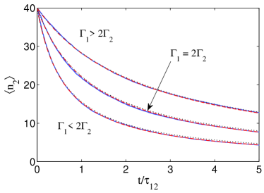
Figure 3: (Color online) Comparison of the two-mode master equation (29) with the single-mode master equation (38) and the analytical approximation of Eq. (45). The solid lines give the two-mode equation, the dashed gives the single-mode, and the dotted – the analytical approximation. Here: $N=40$, $\Gamma_{R}\tau_{12}=200$, and, from the top to bottom, $\Lambda\equiv{UN}/{2J_{12}}=20$, $N/\sqrt{2}$, $40$. To compare the results in the domain of their validity, i.e. after the atoms are removed from mode $b_{1}$, we have used the Fock initial state with all atoms occupying mode $b_{2}$ (a Gaussian with a small dispersion leads to the same results).

V The mean-field approximation

The quantum derivations of the reduced master equations from the first principles, presented above, are involved. One then may inquire if the mean-field approximation, commonly applied to the many-boson models with large number of bosons and which is much simpler to analyze, can substitute the quantum derivation. Here we remind that the two-site model with a local dissipation is perfectly described by the mean-field approximation TWW ; NlZeno . This, however, turns out to be not the case for the three-site Bose-Hubbard model, as we will show below.

The mean-field Hamiltonian can be obtained from Hamiltonian (3) by replacing the boson operators with $c$-numbers ($b_{j}\to\beta_{j}$) BStat , we get

$$\mathcal{H}=-J_{13}(\beta^{*}_{1}\beta_{3}+\beta_{3}^{*}\beta_{1})-J_{12}(\beta^{*}_{1}\beta_{2}+\beta^{*}_{2}\beta_{1})+\varepsilon|\beta_{3}|^{2}$$

$$+U|\beta_{3}|^{4}+\frac{U}{2}\left([|\beta_{1}|^{2}+|\beta_{2}|^{2}]^{2}+[\beta^{*}_{1}\beta_{2}+\beta^{*}_{2}\beta_{1}]^{2}\right).$$ (46)

Note that the total number of atoms is given as $\sum_{j=1}^{3}|\beta_{j}|^{2}=N$. The local atom loss (dissipation) part of Eq. (1) can be simply added to the mean-field Hamiltonian equations as an atom loss of mode $\beta_{3}$ (as we will see shortly, it is describable classically; see also Refs. TWW ; NlZeno ), that is

$$\frac{d\beta_{j}}{dt}=-\frac{i}{\hbar}\frac{\partial\mathcal{H}}{\partial\beta^{*}_{j}}-\delta_{j,3}\frac{\Gamma}{2}\beta_{3}.$$ (47)

Thus, the mean-field equations read:

$$\frac{d\beta_{1}}{dt} = \frac{iJ_{13}}{\hbar}\beta_{3}+\frac{iJ_{12}}{\hbar}\beta_{2}-\frac{iU}{\hbar}(|\beta_{1}|^{2}+2|\beta_{2}|^{2})\beta_{1}$$ (48a)

$$-\frac{iU}{\hbar}\beta^{2}_{2}\beta^{*}_{1},$$

$$\frac{d\beta_{2}}{dt} = \frac{iJ_{12}}{\hbar}\beta_{1}-\frac{iU}{\hbar}(|\beta_{2}|^{2}+2|\beta_{1}|^{2})\beta_{2}-\frac{iU}{\hbar}\beta^{2}_{1}\beta^{*}_{2},\qquad$$ (48b)

$$\frac{d\beta_{3}}{dt} = \frac{iJ_{13}}{\hbar}\beta_{1}-\left(\frac{\Gamma}{2}+\frac{i\varepsilon}{\hbar}\right)\beta_{3}-\frac{2iU}{\hbar}|\beta_{3}|^{2}\beta_{3}.$$ (48c)

V.1 The first reduction: equations for $\beta_{1}$ and $\beta_{2}$

Consider the strongly dissipated case of section III. The small parameter is $\epsilon=\frac{J_{13}}{\hbar\Gamma}$ with the conditions $\frac{J_{12}}{\hbar\Gamma}=\mathcal{O}(\epsilon)$ and $\frac{UN}{\hbar\Gamma}=\mathcal{O}(\epsilon)$. For $t\gg 1/\Gamma$, $\beta_{3}=\mathcal{O}(\epsilon)$ and one can integrate Eq. (48c) by rewriting it in the integral form and neglecting the higher-order nonlinear term. Using the integration by parts, we get

$$\beta_{3}(t)=\frac{2iJ_{13}}{\hbar\Gamma}\left(1+\frac{2i\varepsilon}{\hbar\Gamma}\right)^{-1}\beta_{1}(t)+\mathcal{O}(\epsilon^{2})+\mathcal{O}(e^{-\frac{\Gamma\Delta t}{2}}).$$ (49)

This result corresponds to the expression for the full density matrix (10) with Eqs. (11) and (18), where the amplitude $\beta_{3}$ is locked to that of $\beta_{1}$ and $\beta_{2}$ with the same coefficient as in the full quantum case ($\alpha_{1}$ of Eq. (18)). Eq. (49) can be now inserted into Eqs. (48a) and (48b). We obtain a reduced system describing the coherent modes:

$$\frac{d\beta_{1}}{dt} = -\left(\frac{\Gamma_{R}}{2}+\frac{i\varepsilon_{R}}{\hbar}\right)\beta_{1}+\frac{iJ_{12}}{\hbar}\beta_{2}-\frac{iU}{\hbar}\beta^{2}_{2}\beta^{*}_{1}$$ (50a)

$$- \frac{iU}{\hbar}(|\beta_{1}|^{2}+2|\beta_{2}|^{2})\beta_{1}+\mathcal{O}(\epsilon^{3})+\mathcal{O}(e^{-\frac{\Gamma\Delta t}{2}}),$$

$$\frac{d\beta_{2}}{dt} = \frac{iJ_{12}}{\hbar}\beta_{1}-\frac{iU}{\hbar}(|\beta_{2}|^{2}+2|\beta_{1}|^{2})\beta_{2}-\frac{iU}{\hbar}\beta^{2}_{1}\beta^{*}_{2},\qquad$$ (50b)

where $\Gamma_{R}$ is given by Eq. (20) and the Lamb shift $\varepsilon_{R}$ by Eq. (21) (i.e., by the corresponding quantum results).

V.2 The second reduction: equation for $\beta_{2}$

Now, let us perform the second reduction to an equation for the amplitude $\beta_{2}$, similar as in the quantum case of section IV. In section IV we have assumed that the new small parameter is $\epsilon^{\prime}=\frac{J_{12}}{\hbar\Gamma_{R}}$ with the additional condition on the nonlinearity $\frac{U\langle n_{2}\rangle}{\hbar\Gamma_{R}}=\mathcal{O}(\epsilon^{\prime})$. However, let us for a while broaden the derivation and discard the condition on the nonlinearity. For times $t\gg 1/\Gamma_{R}$ boson mode $\beta_{1}$ is practically empty, i.e. $\beta_{1}=\mathcal{O}(\epsilon^{\prime})$. This allows us to simplify Eqs. (50a) and (50b) as follows

$$\frac{d\beta_{1}}{dt} = -\left[\frac{\Gamma_{R}}{2}+\frac{i\varepsilon_{R}}{\hbar}\right]\beta_{1}+\frac{iJ_{12}}{\hbar}\beta_{2}-\frac{iU}{\hbar}[\beta^{2}_{2}\beta^{*}_{1}+2|\beta_{2}|^{2}\beta_{1}]$$ (51a)

$$+\mathcal{O}({\epsilon^{\prime}}^{3})+\mathcal{O}(e^{-\frac{\Gamma_{R}\Delta t}{2}}),$$

$$\frac{d\beta_{2}}{dt} = \frac{iJ_{12}}{\hbar}\beta_{1}-\frac{iU}{\hbar}|\beta_{2}|^{2}\beta_{2}-\frac{iU}{\hbar}\beta^{2}_{1}\beta^{*}_{2}+\mathcal{O}({\epsilon^{\prime}}^{3})$$ (51b)

$$+\mathcal{O}(e^{-\frac{\Gamma_{R}\Delta t}{2}}),\qquad$$

where, for simplicity, we have dropped the term $\mathcal{O}(\epsilon^{3})$. Already from this system it is clear that the mean-field approach will not account for the boson-pair dissipation channel (41) of mode $b_{2}$, present in the full quantum Eq. (38). Indeed, Eq. (51a) must be somehow integrated with the result to be inserted into Eq. (51b). However, one can notice that the parameter $U$ enters Eq. (51a) only in the conjunction with a factor $\sim|\beta_{2}|^{2}$, hence all the terms in Eqs. (51a) and (51b) scale as $\sqrt{N}$ (the scale of $\beta$) if we fix the nonlinearity parameter $\Lambda=UN$, whereas in the quantum case the $N$-scaling of the boson-pair channel is $\mathcal{O}(1)$.

Now, under the condition on the nonlinearity as in the full quantum case, i.e. $\frac{U\langle n_{2}\rangle}{\hbar\Gamma_{R}}=\mathcal{O}(\epsilon^{\prime})$, one can proceed to derive the reduced equation for the amplitude $\beta_{2}$. To this end, the system of equations for $\beta_{1}$ and $\beta^{*}_{1}$ in the required order can be written in the following form

$$\frac{d}{dt}\left(\begin{matrix}\beta_{1}\\ \beta^{*}_{1}\end{matrix}\right)=\frac{\Gamma_{R}}{2}M\left(\begin{matrix}\beta_{1}\\ \beta^{*}_{1}\end{matrix}\right)+\frac{iJ_{12}}{\hbar}\left(\begin{matrix}\beta_{2}\\ -\beta^{*}_{2}\end{matrix}\right),$$ (52)

where

$$M=\left(\begin{matrix}-\gamma-\frac{4iU}{\hbar\Gamma_{R}}|\beta_{2}|^{2}&-\frac{2iU}{\hbar\Gamma_{R}}(\beta_{2})^{2}\\ \frac{2iU}{\hbar\Gamma_{R}}(\beta^{*}_{2})^{2}&-\gamma^{*}+\frac{4iU}{\hbar\Gamma_{R}}|\beta_{2}|^{2}\end{matrix}\right),$$ (53)

with $\gamma=\left(1+\frac{2i\varepsilon_{R}}{\hbar\Gamma_{R}}\right)$. Eq. (53) can be put into the integral form and integrated for times $t\gg 1/\Gamma_{R}$, in this case the matrix $\frac{\Gamma_{R}}{2}M(t)$ enters the exponent under the integral, with the result

$$\left(\begin{matrix}\beta_{1}\\ \beta^{*}_{1}\end{matrix}\right)=-\frac{2iJ_{12}}{\hbar\Gamma_{R}}M^{-1}\left(\begin{matrix}\beta_{2}\\ -\beta^{*}_{2}\end{matrix}\right)+\mathcal{O}(e^{-\frac{\Gamma_{R}\Delta t}{2}})+\mathcal{O}({\epsilon^{\prime}}^{2}).$$ (54)

We need only the first row of the matrix $M^{-1}$:

$$(M^{-1})_{11}=-\gamma^{-1}+\gamma^{-2}\frac{4iU}{\hbar\Gamma_{R}}|\beta_{2}|^{2}+\mathcal{O}({\epsilon^{\prime}}^{2}),$$ (55)

$$(M^{-1})_{12}=-|\gamma|^{-2}\frac{2iU}{\hbar\Gamma_{R}}(\beta_{2})^{2}+\mathcal{O}({\epsilon^{\prime}}^{2}).$$ (56)

From Eqs. (54)-(56) we obtain

$$\beta_{1}=\gamma^{-1}\frac{2iJ_{12}}{\hbar\Gamma_{R}}\beta_{2}+\mathcal{O}({\epsilon^{\prime}}^{2})+\mathcal{O}(e^{-\frac{\Gamma_{R}\Delta t}{2}}).$$ (57)

Inserting this expression into Eq. (51b) we arrive at the reduced aquation for the amplitude $\beta_{2}$, the mean-field analog of the coherent $\pi$-phase mode $b_{2}$:

$$\frac{d\beta_{2}}{dt} = -\left(\frac{\Gamma_{1}}{2}+\frac{i\varkappa_{1}}{\hbar}\right)\beta_{2}-\frac{iU}{\hbar}|\beta_{2}|^{2}\beta_{2}$$ (58)

$$+\mathcal{O}({\epsilon^{\prime}}^{3})+\mathcal{O}(e^{-\frac{\Gamma_{R}\Delta t}{2}}),$$

with $\Gamma_{1}$ and $\varkappa_{1}$ given in Eq. (37). Observe that, while the single-boson dissipation channel, Eq. (40), is accounted by the mean-field Eq. (58) (the first term on the right hand side), the boson-pair channel, Eq. (41), is not.

In conclusion of this section, we have shown that, while the single-boson dissipation channel of the coherent mode $b_{2}$ can be described by the mean-field approach, the boson-pair dissipation channel cannot be captured by the mean-field approximation and, thus, it has quantum nature.

VI Discussion of the results

We have considered the derivation of the reduced master equations in the limit of strong dissipation on the example of the Bose-Hubbard model with a local external dissipation (i.e., the atom loss from the central site). The method we have used is not based on the assumption of the factorization of the full density matrix, instead we demonstrate that one can effectively solve the master equation directly in the lowest orders of a small parameter (inversely proportional to the local dissipation rate). On this way, one is able to obtain the reduced master equations for the subsystems (the coherent modes) of the higher-order in the small parameter (e.g., we have derived the equation up to the third order).

The derivation reveals the following features. First of all, the full density matrix is not factorized (which is the usual assumption, see for instance Ref. BP ) but is expressed in the form of a “dressed” factorized density matrix, where the population of the strongly dissipated mode depends on that of the other modes. Nevertheless, the reduced density matrix of a subsystem is shown to satisfy a master equation in the Lindblad form. This feature appears in the two reduced master equations derived in the present paper, thus suggesting an universality. Moreover, the Lamb shifts and the dissipation rates of the subsystem turn out to be given by the similar expressions in the two cases, suggesting even the universality of the form of expressions for these quantities.

We have analyzed the relation between the full quantum derivation of the reduced master equation for the density matrix of a subsystem and the mean-field adiabatic elimination procedure. We have found that the mean-field approximation applied to the Bose-Hubbard model cannot capture all dissipation channels of a subsystem, even if the external dissipation applied to the system is describable classically (in our case, the single-boson dissipation channel describing the removal of atoms). Namely, in the three-site Bose-Hubbard model the $\pi$-phase coherent mode has the boson-pair dissipation channel, which is not captured by the mean-field approximation, and the single-boson dissipation, captured by it. This is a quite distinct situation from the two-site model, where the dissipation dynamics is described by the mean-field approximation with a good accuracy TWW ; NlZeno . Here we note, however, that in the two-site model with dissipation the boson-pair tunneling is not possible. Though we have considered the three-site Bose-Hubbard model, the boson-pair dissipation channel is a general feature of the multi-site models, since it is the result of a nonlinearity of the model and the fact that more than one filled site is coupled to the dissipated site, which serves as a common reservoir.

The failure of the mean-field approximation to the quantum master equation means that the dissipation channels not accounted by the mean-field have a genuine quantum nature. This imposes severe limitations on the applicability of the semiclassical mean-field approach to the Bose-Hubbard models considered as open quantum systems, even when the external dissipation is describable classically. Invoking the link to the discrete WKB approach, mentioned in the Introduction, one has to develop a more general approach by going to the first-order approximation in the effective Planck constant $1/N$, i.e. a $1/N$-correction to the mean-filed equations, to capture the boson-pair dissipation channel. This is an important conclusion, in view of the current experiments on the single-site addressability and controlled measurement via the local atom losses of Bose-Einstein condensate loaded in the optical lattices SiteAddr1 ; SiteAddr2 , describable by the open multi-site Bose-Hubbard models.

References

- (1) N. N. Bogoliubov and N. N. Bogoliubov, Jr., Introduction to Quantum Statistical Mechanics (World Scientific Pub Co., 1982).
- (2) L. P. Pitaevskii and S. Stringari, Bose-Einstein Condensates in Gases (Cambridge University Press, Cambridge, England, 2003).
- (3) C. W. Gardiner, Phys. Rev. A 56, 1414 (1997); Y. Castin and R. Dum, Phys. Rev. A 57, 3008 (1998).
- (4) S. Aubry, S. Flach, K. Kladko and E. Olbrich, Phys. Rev. Lett. 76, 1607 (1996).
- (5) G. J. Milburn, J. Corney, E. M. Wright and D. F. Walls, Phys. Rev. A 55, 4318 (1997).
- (6) A. Vardi and J. R. Anglin, Phys. Rev. Lett. 86, 568 (2001).
- (7) J. R. Anglin and A. Vardi, Phys. Rev. A 64, 013605 (2001).
- (8) P. A. Braun, Rev. Mod. Phys. 65, 115 (1993).
- (9) V. S. Shchesnovich and V. V. Konotop, Phys. Rev. A 75, 063628 (2007); ibid 77, 013614 (2008); V. S. Shchesnovich and M. Trippenbach, Phys. Rev. A 78, 023611 (2008).
- (10) V. S. Shchesnovich and V. V. Konotop, Phys. Rev. Lett. 102, 055702 (2009).
- (11) V. S. Shchesnovich, Phys. Rev. A 80, 031601(R) (2009).
- (12) T. Gericke, P. Würtz, D. Reitz, T. Langen, and H. Ott, Nat. Phys. 4, 949 (2008); P. Würtz, T. Langen, T. Gericke, A. Koglbauer, and H. Ott, Phys. Rev. Lett. 103, 080404 (2009).
- (13) W. S. Bakr, J. I. Gillen, A. Peng, S. Fölling, and M. Greiner, Nat. Lett. 462, 74 (2009).
- (14) A. R. Kolovsky and A. Buchleitner, Europhys. Lett. 68, 632 (2004).
- (15) A. R. Kolovsky, Phys. Rev. Lett. 99, 020401 (2007).
- (16) H. Carmichael, An Open Systems Approach to Quantum Optics (Springer, Berlin, 1993).
- (17) H. P. Breuer and F. Petruccione, The Theory of Open Quantum Systems (Oxford University Press, Oxford, 2002).
- (18) F. Trimborn, D. Witthaut, and S. Wimberger, J. Phys. B: At. Mol. Opt. Phys. 41, 171001 (2008).
- (19) V. S. Shchesnovich and V. V. Konotop, Phys. Rev. A 81, 053611 (2010).
- (20) K. Mølmer, Y. Castin and J. Dalibard, J. Opt. Soc. Am. B 10, 524 (1992); H. Carmichael, An Open Systems Approach to Quantum Optics (Springer, Berlin, 1993).
- (21) D. Mogilevtsev, T. Tyc, and N. Korolkova, Phys. Rev. A 79, 053832 (2009).
- (22) P. Lambropoulos, Phys. Rev. 156, 286 (1967); V. V. Dodonov and S. S. Mizrahi, Phys. Lett. A 223, 404 (1996).