The effect of gain saturation in a gain compensated perfect lens

Abstract

The transmission of evanescent waves in a gain-compensated perfect lens is discussed. In particular, the impact of gain saturation is included in the analysis, and a method for calculating the fields of such nonlinear systems is developed. Gain compensation clearly improves the resolution; however, a number of nonideal effects arise as a result of gain saturation. The resolution associated with the lens is strongly dependent on the saturation constant of the active medium.

260.2110, 160.4670, 160.3918.

1 Introduction

Metamaterials have large potential in electromagnetics and optics due to their possibility of tailoring the permittivity and permeability. This enables construction of, for example, media with negative refractive index $n$ [1], perfect lenses [2], invisibility cloaks [3, 4], and other exciting components transforming the electromagnetic field [5]. Unfortunately, the performance of such devices is strongly limited by losses. Although causality and passivity do not prohibit negative index materials with arbitrary low losses [6], in practice it is difficult to fabricate materials with high figure of merit $\text{FOM}=-\text{Re}\,n/\text{Im}\,n$, especially at optical frequencies [7, 8, 9, 10]. For perfect lenses, losses limit the amplification of evanescent waves associated with large spatial frequencies, and therefore the resolution [11, 12]. It has therefore been suggested to introduce gain into the metamaterials [7, 13, 14, 15, 16, 17, 18, 19, 20, 21]. This could be a promising approach provided the intrinsic losses can be made relatively small so that compensation by a realistic amount of gain is possible.

Both permittivity $\epsilon$ and permeability $\mu$ may involve losses; thus in general, gain may be needed to reduce both $\text{Im}\,\epsilon$ and $\text{Im}\,\mu$. For a perfect lens it is generally not sufficient e.g. to reduce $\text{Im}\,\epsilon$ below zero such that the refractive index $n=\sqrt{\epsilon\mu}$ becomes real. However, as long as the object to be imaged is one-dimensional, only one polarization (TE or TM) of the electromagnetic field is required. Then, provided the lens is sufficiently thin, only one of the parameters $\epsilon$ and $\mu$ is relevant for the transmission of evanescent waves [2, 12]. Choosing TM polarization, only $\epsilon$ matters, enabling gain compensation with dielectric, active media.

Introducing the necessary active material into a metamaterial leads to a change not only in the imaginary part but also the real part of the permittivity, and should therefore be kept in mind while designing the metamaterial structure. Other critical considerations include matching of the negative refractive index frequency band to that of the gain lineshape function, the level of loss possible to overcome in the absence of saturation, and the saturation constant of the active medium.

There have been several attempts to create a perfect lens in the near IR-spectrum the last years [7, 8, 9, 22]. The FOM currently reported is of the order of 3 for the frequency where $\text{Re}\,n\approx-1$ [8, 9]. With these values, traditional optical amplifiers such as Erbium-doped silica or gas laser amplifiers will not be able to reduce the intrinsic losses significantly. Theoretical studies have shown that it may be possible to raise the FOM at near IR-frequencies to as much as 20, while keeping $\text{Re}\,n\approx-1$ [23]. It has also been reported that laser dyes, or dye-Ag aggregate mixtures, may reach amplifications of up to $\text{Im}\,n\approx-0.06$ at near IR-frequencies [14, 24]. Taking into account these reports, this article will not speculate further on the choice and design of the metamaterial, but merely assume an appropriate material is physically feasible.

The main purpose of our work is to consider the transmission of evanescent waves in a practical, gain-compensated perfect lens. Clearly, gain saturation is highly relevant in this context, and we demonstrate how this effect leads to limited amplification of evanescent fields, and therefore limited resolution. We calculate the resolution as a function of the saturation constant of the active medium, and also the detailed field profile and reflections from the lens. It will become clear that gain saturation is a critical effect which may lead to severe limitations.

2 Nonlinear gain saturation and field calculations

The relative permittivity of the active metamaterial is given by:

$$\epsilon(\omega)=1+\chi_{\text{p}}(\omega)+\chi_{\text{a}}(\omega),$$ (1)

where $\chi_{\text{p}}(\omega)$ denotes the susceptibility of the passive structure, and $\chi_{\text{a}}(\omega)$ the contribution from the active part. The contribution to the susceptibility for travelling and evanescent fields in active media can be modeled using semiclassical theory [25]. If there is spherical symmetry, allowing for coupling to several degenerate states with different values of the quantum number $m$, one can show using the Wigner-Eckart theorem and the general properties of the Clebsch-Gordan coefficients that the system can effectively be treated as a two-level system. Assuming two-level atoms and using the dipole approximation, we find the following expression for the active susceptibility:

$$\chi_{\text{a}}(\omega)=\frac{A(\omega)\left(\frac{\omega-\omega_{0}}{\gamma}-i\right)}{1+\frac{\left|\mathbf{E}\right|^{2}}{\mathcal{E}_{\text{s}}(\omega)^{2}}}.$$ (2)

Here $\omega_{0}$ is the transition frequency, $\omega$ the frequency of the incident light, $\gamma$ a phenomenological decay rate due to spontaneous emission and elastic collisions, $\mathbf{E}$ the complex electric field, and $\mathcal{E}_{\text{s}}(\omega)$ the saturation constant of the active medium. The saturation constant depends on the selected gain material and pumping level. For dye amplifiers a normal value is $\mathcal{E}_{\text{s}}(\omega_{0})\sim 10^{7}~{}$V$/$m [24, 26], corresponding to intensities in the $\text{kW}/\text{cm}^{2}$ regime for propagating waves. The numerator in Eq. (2) describes the susceptibility in the limit $|\mathbf{E}|/\mathcal{E}_{s}\rightarrow 0$. The numerator contains the line shape function and several material parameters; factors that are irrelevant for the analysis below are absorbed into the function $A(\omega)$. For $\omega=\omega_{0}$ and $|\mathbf{E}|/\mathcal{E}_{s}\rightarrow 0$, $A(\omega)$ is simply $-\text{Im}\,\chi_{\text{a}}(\omega)$. Both functions $A(\omega)$ and $\mathcal{E}_{\text{s}}(\omega)$ are real-valued. Note that the material parameters describing the active medium are effective parameters, depending on the geometry of the metamaterial structure, and are not necessarily equal to the bulk parameters of the gain material [18, 19].

Throughout this paper, we will consider the frequency $\omega=\omega_{0}$. Eq. (2) now reduces to:

$$\chi_{\text{a}}(\omega_{0})=\frac{-iA(\omega_{0})}{1+\frac{\left|\mathbf{E}\right|^{2}}{\mathcal{E}_{\text{s}}(\omega_{0})^{2}}}.$$ (3)

Eq. (3) describes how the imaginary part of the total permittivity relates to the pumping and local field amplitude. The real part of the total permittivity is independent of the pumping and the local field.

Note that there is a fundamental difference between the nonlinearity due to gain saturation, and conventional second- and third-order nonlinearities. First, the nonlinearity due to the denominator in Eq. (2) is so large that a Taylor expansion up third order is generally not valid. Second, the nonlinearity of a gain medium is expressed in terms of the slowly varying field envelope $|\mathbf{E}|$, while the second- and third order nonlinearities usually are expressed in terms of the rapidly varying time-dependent electric field. Since the nonlinearity in our case can be characterized using $|\mathbf{E}|$, the medium will not generate new frequencies for monochromatic input [27]. Nevertheless, if several modes (or frequencies) are present, the modes interact in the sense that the complex refractive index seen by one mode is dependent on the presence and strength of all modes.

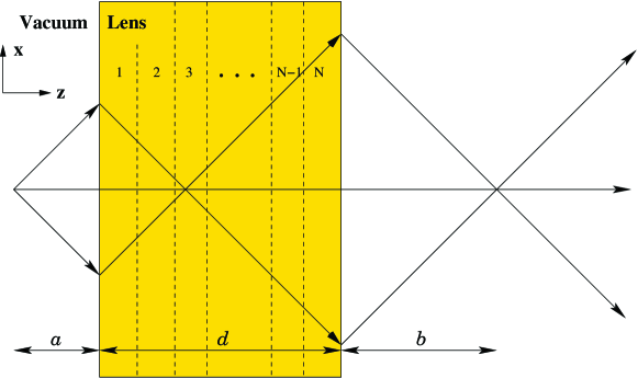
Figure 1: (Color online) Perfect lens in vacuum. The parameter $d$ is the thickness of the lens, $a$ and $b$ are the distances from the source to the lens, and from the lens to the image plane, respectively. The parameters are governed by the equation $d=a+b$. The numbers $1$ through $N$ indicate the different slices. The lens is considered to be infinite in the $xy$-plane. ASHKSF1.eps.

We consider a perfect lens slab which extends to infinity in the $xy$-plane, and has thickness $d$ in the $z$-direction, see Fig. 1. The source is located a distance $a$ (with $a<d$) from the input end of the lens. The incident field from the source will be taken to be a superposition of plane TM-waves, with the magnetic field in the $y$-direction. Provided $\omega_{0}d/c\ll 1$ and $|\mu|\sim 1$, the spesific value of $\mu$ is not critical for the operation of the lens for evanescent waves [2, 12]. Here $c$ is the vacuum light velocity. The permittivity is given by Eqs. (1), (3), and $\text{Re}\,\chi_{\text{p}}(\omega_{0})=-2$. The remaining losses after gain compensation (in the absence of saturation) is described by the parameter:

$$\Delta\chi=\text{Im}\,\chi_{\text{p}}(\omega_{0})-A(\omega_{0}).$$ (4)

To find the steady state solution to Maxwells equations for our nonlinear medium, an iterative approach can be used. In the zeroth iteration, the electric field is simply set to zero everywhere. (Alternatively, the initial field could be set to infinity. This does not give any significant difference in performance, in terms of the required number of iterations.) In the next iteration, Eqs. (1) and (3) are used to find an approximation of the permittivity of the lens. Taking the incident magnetic field to be unity (normalized), we can compute the magnetic and electric fields everywhere. Now we may repeat the iteration; calculate a new approximation of the permittivity from the field, computing the resulting field from this new structure, etc. The iteration procedure has an inherent stability, as growing fields leads to less gain in the medium, and vice versa.

Nevertheless, inaccuracies and even divergence may arise if the number of slices is too low, so that the field no longer can be treated as constant in each slice. In the case $\Delta\chi=0$ the convergence seems to be particularly sensitive to the number of slices. An alternative to increasing the number of slices to a very high number, is to regularize the iterative approach as follows: Rather than setting the permittivity to that resulting from the field in the previous iteration, it can be set to a weighted mean of the permittivities as resulting from the last two iterations. In our computations, the permittivity in iteration $i$ (for $i\geq 2$) was set to 0.5 times the permittivity calculated by the field from iteration $i-1$, pluss 0.5 times that resulting from iteration $i-2$. For $i=1$ the permittivity was calculated using the field from iteration $0$. This resulted in convergence after $\sim 20-35$ iterations. The weight factor 0.5 is somewhat arbitrary; other choices are possible but may require a larger $N$ or number of iterations to obtain convergence.

If the root mean square deviation of three successive iterations are within a specified limit ($10^{-12}$ for the relative permittivity in our computations), and strictly decreasing, the results are deemed converge. Note that when the fields of subsequent iterations coincide, we have a valid solution to Maxwell’s equations with constitute relation as implied by Eqs. (1) and (3).

In general, the fields in one iteration, and therefore the permittivity in the next iteration, will be dependent on $x$ and $z$. Thus the computation of the fields in the next iteration requires the solution to Maxwell’s equations in an inhomogeneous structure. Note that in each iteration, the structure is linear; the nonlinearity of the structure enters through the iteration. For the linear calculation, we employ a transfer matrix technique, considering the different plane waves in the structure. The lens is divided into $N$ slices in the $xy$-plane, as seen in Fig. 1. These slices must be sufficiently thin, such that the permittivity inside each slice is approximately uniform in the $z$-direction. For this condition to be valid for the next iteration as well, the resulting field from the present iteration must also be approximately constant. This means that $k_{x}d/N\lesssim 1$ for the transverse wavenumbers $k_{x}$ that contribute significantly to the fields.

The electric field can be found using the Ampere–Maxwell’s law:

$$\mathbf{E}(x,z)=\frac{1}{-i\omega\epsilon(x,z)\epsilon_{0}}\nabla\times\mathbf{H}(x,z).$$ (5)

With periodic boundary conditions in the $x$-direction, the magnetic field and the permittivity can be expanded in discrete Fourier series

$$\mathbf{H}(x,z)=H(x,z)\mathbf{\hat{y}} = \sum_{m}h_{m}(z)\exp(ik_{xm}x)\mathbf{\hat{y}},$$ (6)

$$\epsilon(x,z) = \sum_{m}e_{m}(z)\exp(ik_{xm}x),$$ (7)

for some Fourier coefficients $h_{m}(z)$ and $e_{m}(z)$. Here $k_{xm}=2\pi m/L$, $L$ is the computational domain, and $\mathbf{\hat{y}}$ is the unit vector in the $y$-direction.

From Maxwell’s equations, we find that the magnetic field satisfies

$$\nabla^{2}H+\epsilon\mu k^{2}H-\frac{1}{\epsilon}\frac{\partial\epsilon}{\partial x}\frac{\partial H}{\partial x}=0,$$ (8)

where $k=\omega_{0}/c$. We express $1/\epsilon$ and $(1/\epsilon)\partial\epsilon/\partial x$ as Fourier series as follows

$$\frac{1}{\epsilon(x)}=\sum_{m}Q_{m}\exp(ik_{xm}x),$$ (9)

and

$$\frac{1}{\epsilon(x)}\frac{\partial\epsilon(x)}{\partial x}=\sum_{m}F_{m}\exp(ik_{xm}x).$$ (10)

The Fourier coefficients $F_{m}$ are now given as

$$F_{m}=\sum_{m^{\prime}}Q_{m-m^{\prime}}ik_{xm^{\prime}}e_{m^{\prime}},$$ (11)

or as a matrix product

$$F=i\mathbf{Q}\mathbf{k_{x}}\mathbf{e},$$ (12)

where $F=\{F_{m}\}_{m}$, $\mathbf{k_{x}}=\mathrm{diag}(k_{xm})$, $\mathbf{e}=\{e_{m}\}_{m}$ and $\mathbf{Q}$ is a Toeplitz matrix with elements $\mathbf{Q}_{i,j}=Q_{i-j}$.

Inserting the Fourier series into equation (8), we obtain

$$\frac{\mathrm{d}^{2}h_{m}(z)}{\mathrm{d}z^{2}}-k_{xm}^{2}h_{m}(z)+k^{2}\mu\sum_{m^{\prime}}\varepsilon_{m-m^{\prime}}(z)h_{m^{\prime}}(z)-\sum_{m^{\prime}}iF_{m-m^{\prime}}k_{xm^{\prime}}h_{m^{\prime}}=0,$$ (13)

for each $m$. Let $\mathbf{h}=\{h_{m}\}_{m\in\mathbb{Z}}$ and use $k_{zm}^{2}=k^{2}-k_{xm}^{2}$. We can write Eq. (13) as a matrix equation

$$\frac{\mathrm{d}^{2}\mathbf{h}(z)}{\mathrm{d}z^{2}}+\left[\mathbf{k_{z}}^{2}+\mathbf{V}\right]\mathbf{h}(z)=0,$$ (14)

where $\mathbf{k_{z}}=\mathrm{diag}(k_{zm})$, and $\mathbf{V}$ is the operator defined as

$$\mathbf{V}=-k^{2}\mathbf{I}+k^{2}\mu\mathbf{G}-\mathbf{F}.$$ (15)

Here $\mathbf{G}$ and $\mathbf{F}$ are infinite dimensional Toeplitz matrices with elements $\mathbf{G}_{i,j}=e_{i-j}$ and $\mathbf{F}_{i,j}=iF_{i-j}k_{xj}$.

Eq. (14) may be decomposed into a first order system by writing $\mathbf{h}=\mathbf{h^{+}}+\mathbf{h^{-}}$, where $\mathbf{h^{+}}=\{h_{m}^{+}\}_{m\in\mathbb{Z}}$ and $\mathbf{h^{-}}=\{h_{m}^{-}\}_{m\in\mathbb{Z}}$. In fact, the equations

$$\frac{\text{d}\mathbf{h^{+}}}{\text{d}z} = i\mathbf{k_{z}}\mathbf{h^{+}}+i(2\mathbf{k_{z}})^{-1}\mathbf{V}(\mathbf{h^{+}}+\mathbf{h^{-}}),$$ (16a)

$$\frac{\text{d}\mathbf{h^{-}}}{\text{d}z} = -i\mathbf{k_{z}}\mathbf{h^{-}}-i(2\mathbf{k_{z}})^{-1}\mathbf{V}(\mathbf{h^{+}}+\mathbf{h^{-}}),$$ (16b)

are seen to be equivalent to (14) after differentiation and summation. This decomposition is particularly convenient, since outside the lens $\mathbf{V}=0$, and Eq. (16) has the simple solution $h_{m}^{\pm}(z)=\text{const}\cdot\exp(\pm ik_{zm}z)$. In other words, outside the lens, $h_{m}^{+}$ and $h_{m}^{-}$ are the forward and backward propagating waves, respectively.

By adding Eqs (16a) and (16b), we obtain

$$\frac{\text{d}\mathbf{h}}{\text{d}z}=i\mathbf{k_{z}}(\mathbf{h^{+}}-\mathbf{h^{-}}),$$ (17)

which is needed for $\nabla\times\mathbf{H}$.

By writing

$$\Psi\mathbf{=}\left[\begin{array}[c]{c}\mathbf{h^{+}}\\ \mathbf{h^{-}}\end{array}\right],\quad\mathbf{C}\mathbf{=}\left[\begin{array}[c]{cc}i\mathbf{k_{z}}+i(2\mathbf{k_{z}})^{-1}\mathbf{V}&i(2\mathbf{k_{z}})^{-1}\mathbf{V}\\ -i(2\mathbf{k_{z}})^{-1}\mathbf{V}&-i\mathbf{k_{z}}-i(2\mathbf{k_{z}})^{-1}\mathbf{V}\\ \end{array}\right],$$ (18)

Eq. (16) may be brought into matrix form:

$$\frac{\text{d}\Psi}{\text{d}z}=\mathbf{C}\Psi.$$ (19)

Since the permittivity is assumed to be independent of $z$ within a slice of the lens, the matrix $\mathbf{C}$ will be constant for each slice. Thus, Eq. (19) can be integrated to obtain

$$\Psi(z_{b})=\exp\{(z_{b}-z_{a})\mathbf{C}\}\Psi(z_{a}),$$ (20)

for $z_{a}$ and $z_{b}$ inside the same slice. Let $z_{j}$ be at the left-hand side of slice $j$, $\Delta_{j}$ the thickness of the slice, and $\mathbf{C}_{j}$ the $\mathbf{C}$-matrix for layer $j$. From the field at $z_{j}$, we find the field at the right hand side of the slice as

$$\Psi(z_{j}+\Delta_{j})=\exp\{\Delta_{j}\mathbf{C}_{j}\}\Psi(z_{j}).$$ (21)

Note that $j=0$ corresponds to the region between the source and the lens, $j=1,...,N$ are the slices inside the lens, and $j=N+1$ represents the region from the lens to the image plane. The thicknesses are $\Delta_{0}=a$, $\Delta_{j}=d/N$, for $j=1,...,N$, and $\Delta_{N+1}=b$. Let us define

$$\mathcal{M}_{j}=\exp\{\Delta_{j}\mathbf{C}_{j}\}.$$ (22)

Eq. (22) propagates the field from the start of a slice, to the end. Next, connecting the fields of adjacent slices with the electromagnetic boundary conditions, we find for the boundary between slice $j$ and $j+1$ that

$$\frac{\partial H_{j+1}(z_{j+1})}{\partial z}=\frac{\epsilon_{j+1}}{\epsilon_{j}}\frac{\partial H_{j}(z_{j+1})}{\partial z}.$$ (23)

Inserting the Fourier series from Eqs. (6) and (7), we obtain a convolution on the right hand side corresponding to the multiplication of a Toeplitz matrix and the vector containing the components $\text{d}h_{m}(z)/\text{d}z$. The Toeplitz matrix is defined by the Fourier components of $\epsilon_{j+1}/\epsilon_{j}$ and will be called $\mathbf{P}$. Then

$$\frac{\text{d}\mathbf{h}_{j}}{\text{d}z}(z_{j+1})=\mathbf{P}_{j}(z_{j+1})\frac{\text{d}\mathbf{h}_{j+1}}{\text{d}z}(z_{j+1}),$$ (24)

where $\mathbf{P}_{j}$ corresponds to the transition between layer $j$ and $j+1$.

Eq. (24) together with the fact that $\mathbf{h}$ is continuous across the layer boundary, gives us the following transfer matrix

$$\left[\begin{array}[c]{c}\mathbf{h^{+}}_{j+1}\\ \mathbf{h^{-}}_{j+1}\end{array}\right]=\frac{1}{2}\left[\begin{array}[c]{cc}\mathbf{I}+\mathbf{k_{z}}^{-1}\mathbf{P}_{j}\mathbf{k_{z}}&\mathbf{I}-\mathbf{k_{z}}^{-1}\mathbf{P}_{j}\mathbf{k_{z}}\\ \mathbf{I}-\mathbf{k_{z}}^{-1}\mathbf{P}_{j}\mathbf{k_{z}}&\mathbf{I}+\mathbf{k_{z}}^{-1}\mathbf{P}_{j}\mathbf{k_{z}}\end{array}\right]\left[\begin{array}[c]{c}\mathbf{h^{+}}_{j}\\ \mathbf{h^{-}}_{j}\end{array}\right].$$ (25)

Let us call the transfer matrix in Eq. (25) $\mathcal{P}_{j}$.

By the successive application of (22) and (25), we find:

$$\left[\begin{array}[c]{c}\mathbf{T}\\ \mathbf{0}\end{array}\right]=\mathcal{M}_{N+1}\prod_{j=N}^{0}(\mathcal{P}_{j}\mathcal{M}_{j})\left[\begin{array}[c]{c}\mathbf{I}\\ \mathbf{R}\end{array}\right].$$ (26)

Here, each column $i$ of $\mathbf{I}$ corresponds to an experiment where the incident field amplitude is 1 for one of the Fourier components and zero for the others. The $i$’th column of $\mathbf{R}$ is the reflection at the source plane of experiment $i$, and the $i$’th column of $\mathbf{T}$ is the corresponding transmission at the image plane. To get the reflection in the case of two or more waves, the corresponding columns of $\mathbf{R}$ are added, the new transmission are found by adding colums of $\mathbf{T}$. Once the total matrix in Eq. (26) has been found, it is straightforward to calculate the unknowns $\mathbf{T}$ and $\mathbf{R}$, and therefore the field amplitudes in all slices.

3 Numerical results

The thickness $d$ of the lens was chosen such that $\omega_{0}d/c=2\pi/10$. The resolution clearly improves with decreasing distance $b$ from the lens to the image, since then the required evanescent fields at the end of the lens are reduced. However there may be practical reasons that makes it impossible to reduce the distances $a$ and $b$ below a certain value. In our simulations we have taken $a=b=d/2$. For simplicity we normalized $\epsilon_{0}=\mu_{0}=\omega_{0}=1$. The permeability was set to $\mu=-1$; however, since the lens was relatively thin, the specific value of $\mu$ did not matter significantly for evanescent TM waves. The number of slices were taken to be $N=20$. The computation domain $L$ was chosen in the range $(15,50)$ depending on the specific problem, and the number of Fourier components ($m$ values) was of the order of $100$.

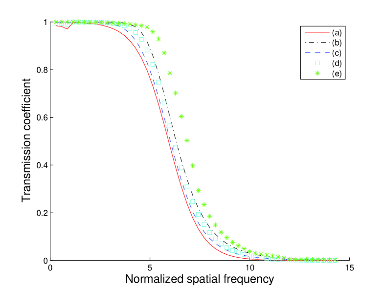
Figure 2: (Color online) The absolute value of the transmission coefficient when $\omega_{0}/c=1$ (normalized), $\omega_{0}d/c=2\pi/10$, $a=b=d/2$, $\text{Im}\,\chi_{\text{p}}(\omega_{0})=0.05$, and $N=20$: ($a$) Non-compensated lens; ($b$) $\mathcal{E}_{\text{s}}=10$, $\Delta\chi=0$; ($c$) $\mathcal{E}_{\text{s}}=4$, $\Delta\chi=0$; ($d$) $\mathcal{E}_{\text{s}}=10$, $\Delta\chi=0.015$; ($e$) $\mathcal{E}_{\text{s}}=10$, $\Delta\chi=0$, two waves, $k_{x}$ and $-k_{x}$, both having amplitude $1/2$. ASHKSF2.eps.

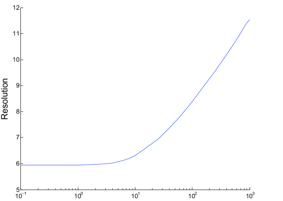
Figure 3: (Color online) The resolution of the lens as a function of the saturation constant. The resolution is defined as the $k_{x}$-value where the transmission equals $1/2$. Parameters: $\omega_{0}/c=1$, $\omega_{0}d/c=2\pi/10$, $\text{Im}\,\chi_{p}(\omega_{0})=0.05$, $\Delta\chi=0$, $a=b=d/2$, and $N=20$. ASHKSF3.eps.

First, a single mode source $\mathbf{H}=\exp(ik_{x}x+ik_{z}z)\mathbf{\hat{y}}$ was considered. The reflection and transmission coefficients, and the fields in the lens, were computed using the iterative method above. The transmission coefficient is shown in Fig. 2. It is easy to see improvements as a result of gain compensation, dependent on the saturation constant $\mathcal{E}_{\text{s}}$. (Here it is useful to recall that for a normalized magnetic field $\mathbf{H}=\exp(ik_{x}x+ik_{z}z)\mathbf{\hat{y}}$, the electric field is $\mathbf{E}=([k_{z}/\omega_{0}\epsilon\epsilon_{0}]\mathbf{\hat{x}}-[k_{x}/\omega_{0}\epsilon\epsilon_{0}]\mathbf{\hat{z}})\exp(ik_{x}x+ik_{z}z)$. Thus, for our normalization, we see that $|\mathbf{E}|\sim k_{x}$, to be compared to $\mathcal{E}_{s}$.) Nevertheless, for a fixed amplitude of the incident field, Fig. 3 indicates that an exponential increase in the saturation constant is needed for a linear increase in the resolution. This is an important result, as it shows the difficulty of getting large resolution: The required, large evanescent fields associated with large spatial frequencies saturate the gain at the output of the lens.

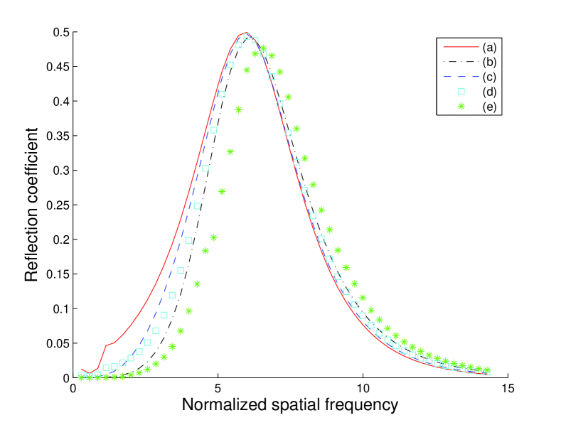
Figure 4: (Color online) The absolute value of the reflection coefficient at the source plane after convergence, for the same cases as those in Fig. 2. ASHKSF4.eps.

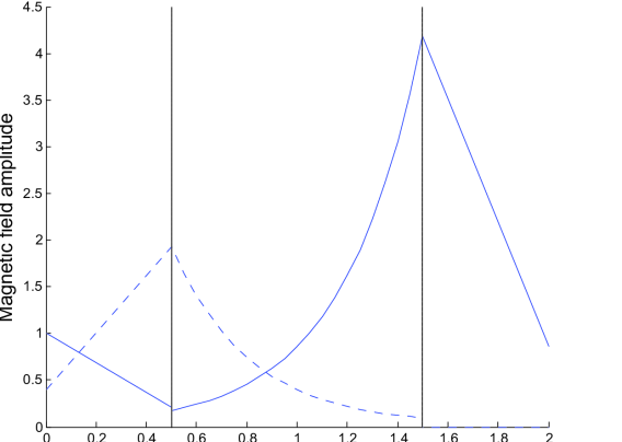
Figure 5: (Color online) The distribution of the two components of the evanescent field in the lens, for one wave with $k_{x}=5.1408$. The distance is normalized with respect to lens thickness, $d$. Parameters: $\omega_{0}/c=1$, $\omega_{0}d/c=2\pi/10$, $\text{Im}\,\chi_{p}(\omega_{0})=0.05$, $\Delta\chi=0$, $\mathcal{E}_{\text{s}}=10$, $a=b=d/2$, and $N=20$. The solid line shows the absolute value of the nonzero component of $\mathbf{h}^{+}$, and the dotted line shows the absolute value of the nonzero component of $\mathbf{h}^{-}$. ASHKSF5.eps.

The reflection coefficient is plotted in Fig. 4. We note that significant reflections arise even for the spatial frequencies where the transmission is relatively large. As can be seen in Fig. 5, the field distributions of the two evanescent components in the lens increase roughly exponentially with $+z$ or $-z$, respectively. For small spatial frequencies, where the lens is essentially perfect, the one increasing in the $+z$ direction dominates. For higher spatial frequencies the two components have a similar amplitude, such that the total field and therefore the imaginary part of the permittivity start to look like a U-shaped valley.

In general, different plane wave components of the source will couple to each other through Eq. (3). To simulate the gain-compensated lens under more real-world conditions, it was therefore tested with several waves traversing the lens simultanously. The transmission of one wave as a function of $k_{x}$, in the presence of another wave $-k_{x}$, is shown in Fig. 2. The amplitudes of both waves were set to $1/2$ to keep the total field at the source equal to the case with a single wave. Moreover, from a number of simulations with several waves, a useful rule of thumb was discovered: As a worst-case estimate, one can judge whether the lens operates as required by assuming that the mode with largest $k_{x}$ has amplitude equal to the sum of the amplitudes at the source. More preciesly, suppose a single mode $k_{x}$ with amplitude $1$ experiences a transmission greater than $1/2$. For any superposition of modes with transversal wavenumbers less than $k_{x}$ and sum of amplitudes equal to unity, each mode will experience a transmission greater than $1/2$.

For conventional lenses, the Rayleigh criterion is usually applied to quantify the distance between two point sources (or in the one-dimensional case, line sources) in order to resolve their images. Since our lens is nonlinear, the image of two line sources cannot be determined as a superposition of the fields associated with the two sources separately, or as a superposition of the fields associated with their Fourier components. Therefore, as in previous literature on perfect lenses, we have chosen to consider a single Fourier component source, and defined the spatial resolution as $2\pi/k_{x}$, where $k_{x}$ is the half maximum wavenumber (Fig. 3). Note that the behavior of the lens for more complex sources can be determined from the rule of thumb described above.

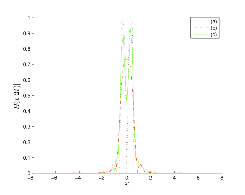
Figure 6: (Color online) The absolute value of the transmitted magnetic field at the image plane, when the source consist of two slits. Parameters: $\omega_{0}/c=1$, $\omega_{0}d/c=2\pi/10$, $\text{Im}\,\chi_{p}(\omega_{0})=0.05$, $\Delta\chi=0$, $a=b=d/2$, and $N=20$: (a) The incident magnetic field at the source, (b) $\mathcal{E}_{s}=0.1$, and (c) $\mathcal{E}_{s}=50$. ASHKSF6.eps.

Fig. 6 shows the absolute value of the transmitted magnetic field at the image plane, $|H(x,2d)|$, resulting from a source consisting of two slits. The image of the slits are clearly better resolved with an increased saturation constant $\mathcal{E}_{s}$.

4 Conclusion

We have developed a method for calculating the transmission, reflection, and detailed field profile of a gain-compensated perfect lens, taking into account gain saturation. The gain compensation clearly improves the resolution limit of perfect lenses. However, due to gain saturation, a number of nonideal effects arise, included limited resolution and reflections. The nonideal effects depend heavily on the saturation constant and/or the field strength of the source.

If there are different waves traversing the lens at the same time, they will interact through the material. Waves with a spatial frequency close to the resolution limit will have the greatest impact. As a rule of thumb, it is enough to know the sum of amplitudes of the waves at the source, and then assume the mode with the largest spatial frequency has this amplitude. If this single wave is transmitted, in the sense of a transmission larger than $1/2$, then so will any superposition of waves with less spatial frequencies and the same sum of amplitudes.

The calculations in this work was performed for TM polarization and a one-dimensional source. For a two-dimensional source with both polarizations, both dielectric and magnetic losses should be compensated, that is, $\text{Im}\,\epsilon$ and $\text{Im}\,\mu$ must be reduced. Although the theory in this paper can trivially be extended to this situation, there may be serious practical problems associated with the fabrication of such active media for optical frequencies.

For a noncompensated lens, the maximum spatial frequency resolved by the lens is approximately $-(1/d)\ln(|1+\epsilon|/2)$ [11, 12]. Thus, for a fixed $d$, an exponential decrease in the losses is necessary to increase the resolution linearly. From our numerical results, a similar relation is approximately valid for the saturation constant of a gain compensated medium; to achieve a linear improvement in the resolution, the saturation constant must increase exponentially. This clearly shows the difficulties of achieving very high resolution.

List of Figure Captions

Fig. 1. (Color online) Perfect lens in vacuum. The parameter $d$ is the thickness of the lens, $a$ and $b$ are the distances from the source to the lens, and from the lens to the image plane, respectively. The parameters are governed by the equation $d=a+b$. The numbers $1$ through $N$ indicate the different slices. The lens is considered to be infinite in the $xy$-plane.

Fig. 2. (Color online) The absolute value of the transmission coefficient when $\omega_{0}/c=1$ (normalized), $\omega_{0}d/c=2\pi/10$, $a=b=d/2$, $\text{Im}\,\chi_{\text{p}}(\omega_{0})=0.05$, and $N=20$: ($a$) Non-compensated lens; ($b$) $\mathcal{E}_{\text{s}}=10$, $\Delta\chi=0$; ($c$) $\mathcal{E}_{\text{s}}=4$, $\Delta\chi=0$; ($d$) $\mathcal{E}_{\text{s}}=10$, $\Delta\chi=0.015$; ($e$) $\mathcal{E}_{\text{s}}=10$, $\Delta\chi=0$, two waves, $k_{x}$ and $-k_{x}$, both having amplitude $1/2$.

Fig. 3. (Color online) The resolution of the lens as a function of the saturation constant. The resolution is defined as the $k_{x}$-value where the transmission equals $1/2$. Parameters: $\omega_{0}/c=1$, $\omega_{0}d/c=2\pi/10$, $\text{Im}\,\chi_{p}(\omega_{0})=0.05$, $\Delta\chi=0$, $a=b=d/2$, and $N=20$.

Fig. 4. (Color online) The absolute value of the reflection coefficient at the source plane after convergence, for the same cases as those in Fig. 2.

Fig. 5. (Color online) The distribution of the two components of the evanescent field in the lens, for one wave with $k_{x}=5.1408$. The distance is normalized with respect to lens thickness, $d$. Parameters: $\omega_{0}/c=1$, $\omega_{0}d/c=2\pi/10$, $\text{Im}\,\chi_{p}(\omega_{0})=0.05$, $\Delta\chi=0$, $\mathcal{E}_{\text{s}}=10$, $a=b=d/2$, and $N=20$. The solid line shows the absolute value of the nonzero component of $\mathbf{h}^{+}$, and the dotted line shows the absolute value of the nonzero component of $\mathbf{h}^{-}$.

Fig. 6. (Color online) The absolute value of the transmitted magnetic field at the image plane, when the source consist of two slits. Parameters: $\omega_{0}/c=1$, $\omega_{0}d/c=2\pi/10$, $\text{Im}\,\chi_{p}(\omega_{0})=0.05$, $\Delta\chi=0$, $a=b=d/2$, and $N=20$: (a) The incident magnetic field at the source, (b) $\mathcal{E}_{s}=0.1$, and (c) $\mathcal{E}_{s}=50$.

References

- [1] V. G. Veselago, “The electrodynamics of substances with simultaneously negative and ”, Sov. Phys. Usp. 10, 509–514 (1968).
- [2] J. B. Pendry, “Negative refraction makes a perfect lens”, Phys. Rev. Lett. 85, 3966–3969 (2000).
- [3] J. B. Pendry and D. Schurig and D. R. Smith, “Controlling electromagnetic fields”, Sience 312, 1780–1782 (2006).
- [4] U. Leonhardt, “Optical conformal mapping”, Science 312, 1777–1780 (2006).
- [5] U. Leonhardt and T. G. Philbin, “General relativity in electrical engineering”, New J. Phys. 8, 247 (2006).
- [6] B. Nistad and J. Skaar, “Causality and electromagnetic properties of active media”, Phys. Rev. E 78, 036603 (2008).
- [7] V. M. Shalaev, “Optical negative-index metamaterials”, Nat. Photonics 1, 41–48 (2007).
- [8] V. M. Shalaev, W. Cai, U. K. Chettiar, H. K. Yuan, A. K. Sarychev, V. P. Drachev and A. V. Kildishev, “Negative index of refraction in optical metamaterials”, Opt. Lett. 24, 3356–3358 (2005).
- [9] G. Dolling, C. Enkrich, M. Wegener, C. M. Soukoulis and S. Linden, “Low-loss negative-index metamaterials at telecommunication wavelengths”, Opt. Lett. 12, 1800–1802 (2006).
- [10] D. H. Kwon, D. H. Werner, A. V. Kildishev and V. M. Shalaev, “Dual-band negative-index metamaterials in the near-infrared frequency range”, in Proceedings of IEEE Antennas and Propagation Society Int. Symp. (IEEE, 2007), pp. 2861–2864.
- [11] S. A. Ramakrishna, J. B. Pendry, D. Schurig, D. R. Smith and S. Schultz, “The asymmetric lossy near-perfect lens”, J. Mod. Optics 49, 1747–1762 (2002).
- [12] Ø. Lind-Johansen, K. Seip and J. Skaar, “The perfect lens on a finite bandwidth”, J. Math. Phys. 50, 012908, (2009).
- [13] S. A. Ramakrishna and J. B. Pendry, “Removal of absorption and increase in resolution in a near-field lens via optical gain”, Phys. Rev. B 67, 201101 (2003).
- [14] M. A. Noginov, G. Zhu, M. Bahoura, J. Adegoke, C. E. Small, B. A. Ritzo, V. P. Drachev and V. M. Shalaev, “Enhancement of surface plasmons in an Ag aggregate by optical gain in a dielectric medium”, Opt. Lett. 31, 3022–3024 (2006).
- [15] A. K. Popov and V. M. Shalaev, “Compensating losses in negative-index metamaterials by optical parametric amplification”, Opt. Lett. 31, 2169–2171 (2006).
- [16] T. A. Klar, A. V. Kildishev, V. P. Drachev and V. M. Shalaev, “Negative-Index Metamaterials: Going Optical”, IEEE J. Sel. Top. Quantum Electron. 12, 1106–1115 (2006).
- [17] J. Zhang, H. Jiang, B. Gralak, S. Enoch, G. Tayeb and M. Lequime, “Compensation of loss to approach -1 effective index by gain in metal-dielectric stacks”, Eur. Phys. J. Appl. Phys. 46, 32603 (2009).
- [18] A. Fang, Th. Koschny, M. Wegener and C. M. Soukoulis, “Self-consistent calculation of metamaterials with gain”, Phys. Rev. B 79, 241104 (2009).
- [19] Y. Sivan, S. Xiao, U. K. Chettiar, A. V. Kildishev and V. M. Shalaev, “Frequency-domain simulations of a negative-index material with embedded gain”, Opt. Express 17, 24060–24074 (2009).
- [20] M. A. Vincenti, D. de Ceglia, V. Rondinone, A. Ladisa, A. D’Orazio, M. J. Bloemer, and M. Scalora, “Loss compensation in metal-dielectric structures in negative-refraction and super-resolving regimes”, Phys. Rev. A 80, 053807 (2009).
- [21] Z. G. Dong, H. Liu, T. Li, Z. H. Zhu, S. M. Wang, J. X. Cao, S. N. Zhu, and X. Zhang, “Optical loss compensation in a bulk left-handed metamaterial by the gain in quantum dots”, Appl. Phys. Lett. 96, 044104 (2010).
- [22] C. Enkrich, M. Wegener, S. Linden, S. Burger, L. Zschiedrich, F. Schmidt, J. F. Zhou, Th. Koschny and C. M. Soukoulis, “Magnetic Metamaterials at Telecommunication and Visible Frequencies”, Phys. Rev. Lett. 95, 203901 (2005).
- [23] S. Zhang, W. Fan, N. C. Panoiu, K. J. Malloy, R. M. Osgood and S. R. J. Brueck, “Optical negative-index bulk metamaterials consisting of 2D perforated metal-dielectric stacks”, Opt. Express 14, 6778–6786 (2006).
- [24] N. M. Lawandy, “Localized surface plasmon singularities in amplifying media”, Appl. Phys. Lett. 21, 5040 (2004).
- [25] M. O. Scully and M. S. Zubairy, “Atom-field interaction - semiclassical theory”, in Quantum Optics, (Cambrigde University Press, 1997), pp. 145–192.
- [26] M. G. Destro and M. S. Zubairy, “Small-signal gain and saturation intensity in dye laser amplifiers”, Appl. Opt. 33, 7007–7011 (1992).
- [27] O. Svelto, Principles of lasers (New York: Plenum Press, 1998).