Parametric Level Set Methods for Inverse Problems

Abstract

In this paper, a parametric level set method for reconstruction of obstacles in general inverse problems is considered. General evolution equations for the reconstruction of unknown obstacles are derived in terms of the underlying level set parameters. We show that using the appropriate form of parameterizing the level set function results a significantly lower dimensional problem, which bypasses many difficulties with traditional level set methods, such as regularization, re-initialization and use of signed distance function. Moreover, we show that from a computational point of view, low order representation of the problem paves the path for easier use of Newton and quasi-Newton methods. Specifically for the purposes of this paper, we parameterize the level set function in terms of adaptive compactly supported radial basis functions, which used in the proposed manner provides flexibility in presenting a larger class of shapes with fewer terms. Also they provide a “narrow-banding” advantage which can further reduce the number of active unknowns at each step of the evolution. The performance of the proposed approach is examined in three examples of inverse problems, i.e., electrical resistance tomography, X-ray computed tomography and diffuse optical tomography.

Keywords: parametric level set methods, shape-based methods, inverse problems
AMS subject classifications: 65J20, 65J22, 65J08
DOI: 10.1137/100800208

1 Introduction

Inverse problems arise in many applications of science and engineering including e.g., geophysics [85, 67], medical imaging [48, 80, 3], nondestructive evaluation [49, 47] and hydrology [82, 13, 71]. In all cases the fundamental problem is usually extracting the information concerning the internal structure of a medium based on indirect observations collected at the periphery, where the data and the unknown are linked via a physical model of the sensing modality. A fundamental challenge associated with many inverse problems is ill-posedness (or ill-conditioning in the discrete case), meaning that the solution to the problem is highly sensitive to noise in the data or effects not captured by the physical model of the sensor. This difficulty may arise due to the underlying physics of the sensing system which in many cases (e.g., electrical impedance tomography [17], diffuse optical tomography [3], inverse scattering [24], etc) causes the data to be inherently insensitive to fine scale variations in the medium. This phenomenon makes such characteristics difficult, if not impossible to recover stably [74]. Another important factor causing the ill-posedness is limitations in the distribution of the sensors yielding sparse data sets that again do not support the recovery of fine scale information uniformly in the region of interest [52]. Many inverse problems of practical interest in fact suffer from both of these problems. From a practical point of view, left untreated, ill-posedness yields reconstructions contaminated by high frequency, large amplitude artifacts.

Coping with the ill-posedness is usually addressed through the use of regularization [53, 27]. Based on prior information about the unknowns, the regularization schemes add constraints to the inverse problem to stabilize the reconstructions. When the inverse problem is cast in a variational framework, these regularization methods often take the form of additive terms within the associated cost function and are interpreted as penalties associated with undesirable characteristics of the reconstruction. They may appear in various forms such as imposing boundedness on the values of the unknown quantity (e.g., Tikhonov or minimum norm regularizations [74, 30]) or penalizing the complexity by adding smoothness terms (e.g., the total variation regularization [1]). These regularization schemes are employed in cases where one seeks to use the data to determine values for a collection of unknowns associated with a dense discretization of the medium (e.g, pixels, voxels, coefficients in a finite element representation of the unknown [63]).

For many problems, the fundamental objective of the process is the identification and characterization of regions of interest in a medium (tumors in the body [12], contaminant pools in the earth [34], cracks in a material sample [70], etc). For such problems, an alternative to forming an image and then post-processing to identify the region is to use the data to directly estimate the geometry of the regions as well as the contrast of the unknown in these regions. Problems tackled in this way are known as the inverse obstacle or shape-based problems. For earlier works in this area see [43, 18, 40] and particularly the more theoretical efforts by Kirsch [39] and Kress et al. [41]. Such processes usually involve a rather simple parametrization of the shape and perform the inversion based on using the domain derivatives mapping the scattering obstacle to the observation. Relative to pixel-type approaches, these geometric formulations tend to result in better posed problems due to a more appropriate obstacle representation. Moreover, in such problems the regularization can be either performed implicitly through the parametrization or expressed in terms of geometric constraints on the shape [44]. However, this class of shape representation is not topologically flexible and the number of components for the shape should be a priori known [64]. They also create difficulties in encountering holes and high curvature regions such as the corners. These difficulties have lead over the past decade or so to the development of shape-based inverse methods employing level set-type representation of the unknowns.

The concept of level sets was first introduced by Osher and Sethian in [57]. This method was initially designed for tracking the motion of a front whose speed depends on the local curvature. The application of the level set approach to inverse problems involving obstacles was discussed by Santosa in [64]. One of the most attractive features of the level set method is its ability to track the motion through topological changes. More specifically, an a priori assumption about the connectedness of the shapes of interest was no longer required. Following Santosa’s work, Litman et al. in [46] explored the reconstruction of the cross-sectional contour of a cylindrical target. Two key distinguishing points about this work were in the way that the authors dealt with the deformation of the contour, and in their use of the level set method to represent the contour. The shape deformation method implemented in this work was enabled by a velocity term, and lead to a closed-form derivative of the cost functional with respect to a perturbation of the geometry. They defined shape optimization as finding a geometry that minimizes the error in the data fit. Later Dorn et al. in [26] introduced a two-step shape reconstruction method that was based on the adjoint field and level set methods. The first step of this algorithm was used as an initialization step for the second step and was mainly designed to deal with the non-linearities present in the model. The second step of this algorithm used a combination of the level set and the adjoint field methods. Although inspired by the works of [57, 64, 46], the level set method used by Dorn et al. was not based on a Hamilton-Jacobi type equation, instead, an optimization approach was employed, and an inversion routine was applied for solving the optimization. The level set ideas in inverse problems were further developed to tackle more advanced problems such as having shapes with textures or multiple possible phases [25, 15]. Moreover, regarding the evolution of the level set function where usually gradient descent methods are the main minimization schemes applied, some authors such as Burger [10] and Soleimani [68] proposed using second order convergent methods such as the Newton and quasi-Newton methods.

Although level set methods provide large degrees of flexibility in shape representation, there are numerical concerns associated with these methods. Gradient descent methods used in these problems usually require a long evolution process. Although this problem may be overcome using second order methods, the performance of these methods for large problems such as 3D shape reconstructions remains limited and usually gradient descent type methods are the only option for such problems. Moreover re-initialization of the level set function to keep it well behaved and velocity field extensions to globally update the level set function through the evolution are usually inevitable and add extra computational costs and complexity to the problem [56]. More detailed reviews of level set methods in inverse problems can be found in [24, 11].

In all traditional level set methods already stated, the unknown level set function belongs to an infinite dimensional function space. From an implementation perspective, this requires the discretization of the level set function onto a dense collection of nodes. An alternative to this approach is to consider a finite dimensional function space or a parametric form for the level set function such as the space spanned by a set of basis functions. Initially, Kilmer et al. in [38] proposed using a polynomial basis for this purpose in diffuse optical tomography applications. In this approach, the level set function is expressed in terms of a fixed order polynomial and evolved through updating the polynomial coefficients at every iteration. Parametrization of the level set function later motivated some authors in field of mechanics to use it in applications such as structural topology optimization [79, 78, 61]. One of the main contributions in this regard is the work by Wang et al. in [79]. Here the level set function is spanned by multiquadric radial basis functions as a typical basis set in scattered data fitting and interpolation applications. Authors showed that through this representation, the Hamilton-Jacobi partial differential equation changes into a system of ordinary differential equations and the updates for the expansion coefficients may be obtained by numerically solving an interpolation problem at every iteration.

More recently, the idea of parametric representation of the level set function has been considered for image processing applications [29, 5]. Gelas et al. in [29] used a similar approach as the one by Wang et al. for image segmentation. As the basis set they used compactly supported radial basis functions, which not only reduce the dimensionality of the problem due to the parametric representation, but also reduce the computation cost through the sparsity that this class of functions provide. As advantages of the method they showed that appropriate constraints on the underlying parameters can avoid implementation of the usual re-initialization. Also the smoothness of the solution is guaranteed through the intrinsic smoothness of the underlying basis functions, and in practice no further geometric constraints need to be added to the cost function. As an alternative to this approach, Bernard et al. in [5] parameterized the level set function in terms of B-splines. One of the main advantages of their method was representing the the cost function minimization directly in terms of the B-spline coefficients and avoiding the evolution through the Hamilton-Jacobi equation.

In this paper the general parametric level set approach for inverse problems is considered. For an arbitrary parametrization of the level set function, the evolution equation is derived in terms of the underlying parameters. Since one of the main advantages of this approach is low order representation of the level set function, in practice the number of unknown parameters in the problem is much less than the number of pixels (voxels) in a traditional Hamilton-Jacobi type of level set method, therefore we concentrate on faster converging optimization methods such as the Newton or quasi-Newton type method. To represent the parametric level set function, as in [79, 29] we have proposed using radial basis functions. However unlike the previous works employing radial basis functions in a level set framework, in addition to the weighting coefficients, the representation is adaptive with respect to the centers and the scaling of the underlying radial basis functions. This technique basically prevents using a large number of basis terms in case that no prior information about the shape is available. To fully benefit from this adaptivity, we further narrow our choice by considering compactly supported radial basis functions. Apparently, this choice would result sparsity in the resulting matrices. However, we will discuss a behavior of these functions which can be exploited to further reduce the number of underlying basis terms and provide the potential to reconstruct rather high curvature regions. The flexibility and performance of proposed methods will be examined through illustrative examples.

The paper is structured as follows. In Section 2 we review shape-based inverse problems in a general variational framework. Section 3 is concerned with obtaining the first and second order sensitivities of the cost function with respect to the functions defining the shape. Based on the details provided, a brief revision of the relevant traditional level set methods is provided paving the path to use parametric level set methods. In Section 4 the general parametric level set method will be introduced and evolution equations corresponding to the underlying parameters are derived. In Section 5 an adaptive parametric level set based on the radial basis functions will be proposed and the approach will be narrowed down to compactly supported class of functions, due to their interesting properties. Section 6 will examine the method through some examples in the context of electrical resistance tomography, X-ray tomography and diffuse optical tomography. Finally in Section 7 some concluding remarks and suggestions will be provided.

2 Problem Formulation

2.1 Forward Modelling

The approach to modelling and determination of shape we consider in this paper is rather general with the capability of being applied to a range of inverse problems. In Section 6 we specifically consider three applications: electrical resistance tomography, limited view X ray tomography, and diffuse optical tomography. The details of the specific problems will be provided in the same section within the context of the examples themselves. Up until that point, we have chosen to keep the discussion general.

Consider $\Omega$ to be a compact domain in $\mathbb{R}^{n}$, $n\geq 2$, with Lipschitz boundary $\partial\Omega$. Further assume for $\mathbf{x}\in\Omega$, a space dependent property $p(\mathbf{x})\in\mathbb{S}_{p}$, where $\mathbb{S}_{p}$ is a Hilbert space. A physical model $\mathcal{M}$ acts on a property of the medium (e.g., electrical conductivity, mass density or optical absorption), $p$, to generate an observation (or measurement) vector $u$,

$$u=\mathcal{M}(p),$$ (1)

where $u$ itself belongs to some Hilbert space $\mathbb{S}_{u}$. In most applications $u$ is a vector in $\mathbb{C}^{k}$, the space of $k$ dimensional complex numbers where $k$ represents the number of measurements and accordingly a canonical inner product is used.

As a convention throughout this paper, to keep the generality of notation, the inner products and norms corresponding to any Hilbert space $\mathbb{H}$, are subindexed with the notation of the space itself, e.g. $\langle.,.\rangle_{\mathbb{H}}$.

2.2 Inverse Problem

The goal of an inverse problem is the recovery of information about the property $p$ based on the data $u$. Here we consider a variational approach where the estimate of $p$ is generated as the solution to an optimization problem. The functional underlying the problem is usually comprised of two terms. The first term demands that the estimate of $p$ be consistent with the data in a mathematically precise sense. As is well known however, many interesting inverse problems are quite ill-posed. This means when the data consistency is our only concern, the resulting estimate of $p$ could be quite far from the truth, corrupted by artifacts such as high frequency and large amplitude oscillations. Hence, an additional term (or terms) are required in the formulation of the variation problem which capture our prior knowledge concerning the expected behavior of the $p$ in $\Omega$. Such terms serve to stabilize (or regularize) the inverse problem. Defining a residual operator as

$$\mathcal{R}(p)=\mathcal{M}(p)-u,$$ (2)

the inverse problem is formulated in the following manner

$$\underset{p}{\min}\>\ \mathscr{F}(p)=\frac{1}{2}\|\mathcal{R}(p)\|_{\mathbb{S}_{u}}^{2}+\mathscr{L}\!(p),$$ (3)

where $\mathscr{L}$ is the regularization functional. Appropriate choice of $\mathscr{L}$ is usually based on properties of the problem. In the typical case where the unknown property $p$ is represented as a dense collection of pixels (or voxels) in $\Omega$, the regularization penalties are used to enforce smoothness and boundedness of $p$ in $\Omega$. These are usually considered in the framework of Tikhonov and total variation regularizations [74, 1]. An alternative approach that has been of great interest in recent years is based on geometric parameterizations of the unknown. Here the regularization penalties are either embedded in the nature of the unknown or expressed as geometric constraints on the unknown. No matter which approach is used, usually in defining $\mathscr{L}$ different spaces and their corresponding norms may be used. For a more detailed review of such methods an interested reader is referred to [77, 24]. Clearly when the number of parameters involved in the problem is sufficiently small, an underdetermined inverse problem can be made overdetermined, and in this sense the problem becomes better posed. Since the parametrization idea we will put forth in this paper is empirically found to be well-posed enough that no necessary regularization terms need to be added to the cost function, $\mathscr{L}$ will be neglected in our future discussions of $\mathscr{F}$.

2.3 A Shape-Based Approach For the Unknown Parameter

For a large class of “shape-based” inverse problems [64, 42, 24, 51], it is natural to view $p(\mathbf{x})$ as being comprised of two classes, i.e., foreground and background. The problem then amounts to determination of the boundary separating these classes as well as characteristics of the property values in each class. In the simplest case, $p(\mathbf{x})$ is piecewise constant while in more sophisticated cases $p(\mathbf{x})$ may be random and characterized by different probabilistic models in the two regions. In this paper, we assume that over each region $p(\mathbf{x})$ is at least differentiable. The property of interest in this case is usually formulated through the use of a characteristic function. Given a closed domain $D\subseteq\Omega$ with corresponding boundary $\partial D$, the characteristic function $\chi_{D}$ is defined as

$$\chi_{D}(\mathbf{x})=\left\{\begin{array}[]{rl}1&\mathbf{x}\in D\\ 0&\mathbf{x}\in\Omega\setminus D.\\ \end{array}\right.$$ (4)

Accordingly, the unknown property $p(\mathbf{x})$ can be defined over the entire domain $\Omega$ as

$$p(\mathbf{x})=p_{i}(\mathbf{x})\chi_{D}(\mathbf{x})+p_{o}(\mathbf{x})\big{(}1-\chi_{D}(\mathbf{x})\big{)}.$$ (5)

Unlike $p(\mathbf{x})$ which is clearly not differentiable along $\partial D$, $p_{i}(\mathbf{x})$ indicating the property values inside $D$ and $p_{o}(\mathbf{x})$ denoting the values outside, are assumed to be smooth functions, and as mentioned earlier, at least belonging to $C^{1}(\Omega)$.

In a shape-based approach, finding $\partial D$ is a major objective. As (5) and (4) show, $p(\mathbf{x})$ is implicitly related to $D$ and to find $\partial D$, a more explicit way of relating them should be considered. In this regard the idea of using a level set function proves to be especially useful [64]. Here $\partial D$ is represented as some level set of a Lipschitz continuous function $\phi:\Omega\rightarrow\mathbb{R}$. When the zero level set is considered, $\phi(\mathbf{x})$ is related to $D$ and $\partial D$ via

$$\left\{\begin{array}[]{rl}\phi(\mathbf{x})>0&\forall\mathbf{x}\in D\\ \phi(\mathbf{x})=0&\forall\mathbf{x}\in\partial D\\ \phi(\mathbf{x})<0&\forall\mathbf{x}\in\Omega\setminus D.\\ \end{array}\right.$$ (6)

Making the use of a Heaviside function, defined as $H(.)=\frac{1}{2}\big{(}1+\operatorname{sign}(.)\big{)}$, the function $p(\mathbf{x})$ can be represented as

$$p(\mathbf{x})=p_{i}(\mathbf{x})H\big{(}\phi(\mathbf{x})\big{)}+p_{o}(\mathbf{x})\Big{(}1-H\big{(}\phi(\mathbf{x})\big{)}\Big{)}.$$ (7)

This equation in fact maps the space of unknown regions $D$ into the space of unknown smooth functions $\phi$.

3 Inversion as a Cost Function Minimization

In this section we develop the mathematical details of the minimization problem (3) when a shape-based approach as (7) is considered. Most current methods use the first and second order sensitivities of the cost function with respect to the unknown parameter to perform the minimization [11]. Based on the general details provided, we will briefly revisit the traditional level set approaches relevant to this paper in Section 3.2, since understanding the details better justifies the use of parametric level set methods.

3.1 Cost Function Variations Due to the Unknowns

We begin by assuming that the first and second order Fréchet derivatives of $\mathcal{R}(p)$ exist and denote them as $\mathcal{R}^{\prime}(p)[\hskip 1.99168pt.\hskip 1.99168pt]$ and $\mathcal{R}^{\prime\prime}(p)[.,.]$. The first order Fréchet derivative of a function (if it exists) is a bounded and linear operator. The second order Fréchet derivative is also bounded but bilinear, which means the operator acts on two arguments and is linear with respect to each [4].

For an arbitrary variation $\delta p\in\mathbb{S}_{p}$ and the real scalar $\varepsilon$, using the generalized Taylor expansion we have

$$\mathcal{R}(p+\varepsilon\delta p)=\mathcal{R}(p)+\varepsilon\mathcal{R}^{\prime}(p)[\delta p]+\frac{\varepsilon^{2}}{2}\mathcal{R}^{\prime\prime}(p)[\delta p,\delta p]+O(\varepsilon^{3}).$$ (8)

Rewriting $\mathscr{F}(p)$ as

$$\mathscr{F}(p)=\frac{1}{2}\langle\mathcal{R}(p),\mathcal{R}(p)\rangle_{\mathbb{S}_{u}},$$ (9)

and recalling the fact that $\langle u_{1},u_{2}\rangle_{\mathbb{S}_{u}}=\overline{\langle u_{2},u_{1}}\rangle_{\mathbb{S}_{u}}$ for $u_{1},u_{2}\in\mathbb{S}_{u}$ and overline denoting complex conjugate, the variations of the cost function with respect to the variations of $p$ can be derived as

$$\mathscr{F}(p+\varepsilon\delta p)=\mathscr{F}(p)+\varepsilon\mathscr{F}^{\prime}(p)[\delta p]+\frac{\varepsilon^{2}}{2}\mathscr{F}^{\prime\prime}(p)[\delta p,\delta p]+O(\varepsilon^{3}),$$ (10)

where for $p_{1},p_{2}\in\mathbb{S}_{p}$

$$\mathscr{F}^{\prime}(p)[p_{1}]=\mathscr{R}\!\mathpzc{e}\langle\mathcal{R}^{\prime}(p)[p_{1}],\mathcal{R}(p)\rangle_{\mathbb{S}_{u}}$$ (11)

and

$$\mathscr{F}^{\prime\prime}(p)[p_{1},p_{2}]=\mathscr{R}\!\mathpzc{e}\langle\mathcal{R}^{\prime}(p)[p_{1}],\mathcal{R}^{\prime}(p)[p_{2}]\rangle_{\mathbb{S}_{u}}+\mathscr{R}\!\mathpzc{e}\langle\mathcal{R}^{\prime\prime}(p)[p_{1},p_{2}],\mathcal{R}(p)\rangle_{\mathbb{S}_{u}}.$$ (12)

The notation $\mathscr{R}\!\mathpzc{e}$ indicates the real part of the corresponding quantity. Denoting $\mathcal{R}^{\prime}(p)^{*}[\;.\;]$ as the adjoint operator between $\mathbb{S}_{u}$ and $\mathbb{S}_{p}$ as

$$\langle\hat{u},\mathcal{R}^{\prime}(p)[\hat{p}]\rangle_{\mathbb{S}_{u}}=\langle\mathcal{R}^{\prime}(p)^{*}[\hat{u}],\hat{p}\rangle_{\mathbb{S}_{p}},\qquad\forall\hat{u}\in\mathbb{S}_{u},\forall\hat{p}\in\mathbb{S}_{p},$$ (13)

(11) can be written as

$$\mathscr{F}^{\prime}(p)[p_{1}]=\mathscr{R}\!\mathpzc{e}\langle\mathcal{R}^{\prime}(p)^{*}[\mathcal{R}(p)],p_{1}\rangle_{\mathbb{S}_{p}}.$$ (14)

Equations (11), (14) and (12) are in fact the first and second order Fréchet derivatives of $\mathscr{F}$ with respect to $p$. In a more general context (and indeed one which we shall use in Section 4), $p$ itself can be the map over some variable $v$ from another Hilbert space $\mathbb{S}_{v}$ into $\mathbb{S}_{p}$, i.e., $p(v):\mathbb{S}_{v}\rightarrow\mathbb{S}_{p}$. Assuming the existence of the first and second order Fréchet derivatives of $p$ with respect to $v$, denoted as $p^{\prime}(v)[\hskip 1.99168pt.\hskip 1.99168pt]$ and $p^{\prime\prime}(v)[.,.]$, the first and second order Fréchet derivatives of $\mathscr{F}$ with respect to $v$ can be obtained using the chain rule as

$$\mathscr{F}^{\prime}(v)[v_{1}]=\mathscr{F}^{\prime}(p)\big{[}p^{\prime}(v)[v_{1}]\big{]}$$ (15)

and

$$\mathscr{F}^{\prime\prime}(v)[v_{1},v_{2}]=\mathscr{F}^{\prime\prime}(p)\big{[}p^{\prime}(v)[v_{1}],p^{\prime}(v)[v_{2}]\big{]}+\mathscr{F}^{\prime}(p)\big{[}p^{\prime\prime}(v)[v_{1},v_{2}]\big{]},$$ (16)

where $v_{1},v_{2}\in\mathbb{S}_{v}$. Equations (15) and (16) themselves can be easily expressed in terms of $\mathcal{R}(p)$ and its derivatives using (11) and (12). These equations will be used later as the key equations in finding the sensitivities in our parametric level set representation of $p$.

3.2 Pixel Based Minimizations (Revisiting Traditional Level Set Methods)

In the specific context of the shape-based inverse problems of interest here, the first and second order sensitivities of the cost function $\mathscr{F}$ with respect to the functions defining $p(\mathbf{x})$ in (7) i.e., $\phi(\mathbf{x})$, $p_{i}(\mathbf{x})$ and $p_{o}(\mathbf{x})$, can be used to form a minimization process. Based on the order of the sensitivities available, first order optimization methods such as gradient descent or second order methods such as Newton or quasi-Newton techniques can be implemented.

For simplicity in reviewing the current methods, we assume that $p_{i}$ and $p_{o}$ are known a priori and only the shape (i.e., the zero level set of $\phi$) is unknown (see [76, 28, 25] for details on the recovery of both the shape as well as the contrast function). In an evolution approach it is desired to initialize a minimization process with some level set function $\phi_{0}$ and evolve the function to find a $\phi$ which minimizes $\mathscr{F}$. To take into account the concept of evolution, an artificial time is defined where the level set function at every time frame $t\geq 0$ is rewritten as $\phi(\mathbf{x};t)$ and the zero level set of $\phi(\mathbf{x};t)$ is denoted as $\partial D_{t}$. A straightforward differentiation of $\phi(\mathbf{x};t)=0$ with respect to $t$ yields to the Hamilton-Jacobi type equation

$$\frac{\partial\phi}{\partial t}+V(\mathbf{x};t)\cdot\nabla\phi=0$$ (17)

for the points on $\partial D_{t}$ where $V(\mathbf{x};t)=\mbox{d}\mathbf{x}/\mbox{d}t$. To move the interface in the normal direction, $V(\mathbf{x};t)$ should be chosen as $v(\mathbf{x};t)\vec{n}(\mathbf{x};t)$ where $v$ is a scalar speed function and $\vec{n}=\nabla\phi/|\nabla\phi|$ is the unit outward vector on $\partial D_{t}$. Incorporating this into the minimization of $\mathscr{F}$, the speed function for the points on $\partial D_{t}$, denoted as $\tilde{v}$, can be chosen to be in the steepest descent direction of $\mathscr{F}$ which is [24]

$$\tilde{v}=-\mathscr{R}\!\mathpzc{e}\{(p_{o}-p_{i})\overline{\mathcal{R}^{\prime}(p)^{*}\left[\mathcal{R}(p)\right]}\}.$$ (18)

As (18) is only valid for $\mathbf{x}\in\partial D$, a velocity extension should be performed to extend $\tilde{v}$ to $v$ defined over the entire domain $\Omega$ and therefore capable of globally evolve the level set function [56]. Beside this classical level set approach, other ways of representing the speed functions and performing the minimization process are proposed [50, 10, 58]. For example, Hadj Miled and Miller [50] proposed a normalized version of the classic speed function in the context of electrical resistance tomography.

Some authors have also proposed using Newton type methods to update $\tilde{v}$ at every iteration (e.g., see [64, 10, 69]). Analogous to (2) and (9), in these problems the residual operator and the cost function are usually written directly as $\mathcal{R}(D)$ and $\mathscr{F}(D)$, functions of the shape itself. Assuming the existence of the first and second order shape derivatives [55], denoted as $\mathscr{F}^{\prime}(D)[\hskip 1.99168pt.\hskip 1.99168pt]$ and $\mathscr{F}^{\prime\prime}(D)[.,.]$, at every time step the Newton update $\tilde{v}$ is obtained by solving [11]

$$\mathscr{F}^{\prime\prime}(D)[w,\tilde{v}]+\mathscr{F}^{\prime}(D)[w]=0\qquad\forall w\in\mathbb{S}_{D}.$$ (19)

Here $\mathbb{S}_{D}$ is an appropriate Hilbert space such as $L^{2}(\partial D)$, which may depend on the current shape [10, 9]. Considering the general forms of the derivatives as (11) and (12), in a Gauss-Newton method the second derivatives of $\mathcal{R}$ are disregarded and (19) becomes

$$\mathscr{R}\!\mathpzc{e}\langle\mathcal{R}^{\prime}(D)[\tilde{v}],\mathcal{R}^{\prime}(D)[w]\rangle_{\mathbb{S}_{u}}+\mathscr{R}\!\mathpzc{e}\langle\mathcal{R}^{\prime}(D)[w],\mathcal{R}(D)\rangle_{\mathbb{S}_{u}}=0\qquad\forall w\in\mathbb{S}_{D}.$$ (20)

Furthermore, to avoid ill conditioning, in a Levenberg-Marquardt approach (20) is regularized as

$$\mathscr{R}\!\mathpzc{e}\langle\mathcal{R}^{\prime}(D)[\tilde{v}],\mathcal{R}^{\prime}(D)[w]\rangle_{\mathbb{S}_{u}}+\mathscr{R}\!\mathpzc{e}\langle\mathcal{R}^{\prime}(D)[w],\mathcal{R}(D)\rangle_{\mathbb{S}_{u}}+\lambda\langle\tilde{v},w\rangle_{\mathbb{S}_{D}}=0\qquad\forall w\in\mathbb{S}_{D}.$$ (21)

in which for $\lambda>0$, the equation is shown to be well-posed [10]. Similar to the previous approach, once $\tilde{v}$ is obtained, a velocity extension is performed to result a globally defined $v$ which can be used to update $\phi$. However, although using second order methods can reduce the number of iterations in finding a minima, compared to gradient descent methods, they do not necessarily reduce the computation load.

From an implementation perspective there are some concerns using the aforementioned methods. The gradient descent method usually requires many iterations to converge and performances become poor for low sensitivity problems [50]. Although using Newton and quasi-Newton methods to update the level set function increases the convergence rate, they are usually computationally challenging and for large problems and relatively finer grids, a large system of equations must be solved at every iteration. Also for both types of methods, there are usually added complications of the level set function re-initialization and speed function extension. The approach that we will put forth in the next section is capable of addressing these problems. It is low order and numerically speaking, the number of unknowns involved in the problem are usually much less than the number of grid points and hence allows us to easily use second order methods. Moreover, our proposed method does not require re-initialization of the level set function, speed function extension or even length-type regularization as a common regularization in many shape-based methods (e.g., see [33, 50, 24]) and our level set function remains well behaved through the corresponding evolution process.

4 A Parametric Level Set Approach

As discussed earlier, in most current shape-based methods $\phi(\mathbf{x})$ is represented by function values on a dense discretization of $\mathbf{x}$-space as part of a discretization of the underlying evolution equation or Newton-type algorithm. Consider now the level set function to be still a function of $\mathbf{x}$ but also a function of a parameter vector $\boldsymbol{\mu}=(\mu_{1},\mu_{2},\cdots,\mu_{m})\in\mathbb{R}^{m}$. In this case we define the continuous Lipschitz function $\phi:\Omega\times\mathbb{R}^{m}\rightarrow\mathbb{R}$, as a parametric level set (PaLS) representation of $D$ if for a $c\in\mathbb{R}$

$$\left\{\begin{array}[]{rl}\phi(\mathbf{x},\boldsymbol{\mu})>c&\forall\mathbf{x}\in D\\ \phi(\mathbf{x},\boldsymbol{\mu})=c&\forall\mathbf{x}\in\partial D\\ \phi(\mathbf{x},\boldsymbol{\mu})<c&\forall\mathbf{x}\in\Omega\setminus D.\\ \end{array}\right.$$ (22)

In the PaLS approach we assume that the general form of $\phi(\mathbf{x},\boldsymbol{\mu})$ is known and the specification of $\boldsymbol{\mu}$ can explicitly define the level set function over the entire domain $\Omega$. In other words the evolution of $\phi$ required to solve the underlying inverse problems is performed via the evolution of $\boldsymbol{\mu}$. An example of a PaLS function is a basis expansion with known basis functions and unknown weights and as will be shown later in this paper we considerably expand on this notion. We call $\boldsymbol{\mu}$ the PaLS parameters.

To setup the problem using the PaLS approach, consider momentarily that $p_{i}(\mathbf{x})$ and $p_{o}(\mathbf{x})$ are known a priori (later we will appropriately take away this restriction). Based on (22) $p$ is written as

$$p(\mathbf{x},\boldsymbol{\mu})=p_{i}(\mathbf{x})H\big{(}\phi(\mathbf{x},\boldsymbol{\mu})-c\big{)}+p_{o}(\mathbf{x})\Big{(}1-H\big{(}\phi(\mathbf{x},\boldsymbol{\mu})-c\big{)}\Big{)}.$$ (23)

Under this model, we now view $\mathscr{F}$ in (9) as a function of $\boldsymbol{\mu}$, i.e. $\mathscr{F}(\boldsymbol{\mu}):\mathbb{R}^{m}\rightarrow\mathbb{R}$. Therefore unlike the classic level set approach, the unknown is no longer the function $\phi$, but a vector belonging to $\mathbb{R}^{m}$, where $m$ is usually much smaller than the number of unknowns associated with a discretization of $\mathbf{x}$-space. With this model and assuming (1) $\phi$ is sufficiently smooth with respect to the elements of $\boldsymbol{\mu}$ and (2) the discontinuous Heaviside function is replaced by a $C^{2}$ approximation (e.g., [84]) denoted as $H_{rg}$, we now proceed to formulate a second order approach for the minimization of $\mathscr{F}(\boldsymbol{\mu})$. To begin, rewriting (23) with $H_{rg}$ and taking a derivative with respect to $\phi$ yields

$$\frac{\partial p}{\partial\phi}=(p_{i}-p_{o})\delta_{rg}(\phi-c),$$ (24)

where $\delta_{rg}(.)$ is accordingly the regularized version of the Dirac delta function (see examples in [73, 84]). Using the chain rule gives

$$\frac{\partial p}{\partial\mu_{j}}=\frac{\partial p}{\partial\phi}\frac{\partial\phi}{\partial\mu_{j}}=(p_{i}-p_{o})\delta_{rg}(\phi-c)\frac{\partial\phi}{\partial\mu_{j}}.$$ (25)

Now using (25) with (15) and (14), the gradient vector for $\mathscr{F}$ is

$$\frac{\partial\mathscr{F}}{\partial{\mu_{j}}} =\mathscr{F}^{\prime}(p)[\frac{\partial p}{\partial\mu_{j}}]$$

$$=\mathscr{R}\!\mathpzc{e}\langle\mathcal{R}(p),\mathcal{R}^{\prime}(p)[\frac{\partial p}{\partial\mu_{j}}]\rangle_{\mathbb{S}_{u}}$$ (26)

$$=\mathscr{R}\!\mathpzc{e}\langle\mathcal{R}^{\prime}(p)^{*}[\mathcal{R}(p)],(p_{i}-p_{o})\delta_{rg}(\phi-c)\frac{\partial\phi}{\partial\mu_{j}}\rangle_{\mathbb{S}_{p}}.$$ (27)

We denote by $\mathbf{J}_{\boldsymbol{\mu}}(\mathscr{F})$ the gradient of $\mathscr{F}$ with respect to the parameter vector $\boldsymbol{\mu}$. With this notation a gradient descent equation can be formed to evolve the PaLS function as

$$\boldsymbol{\mu}^{(t+1)}=\boldsymbol{\mu}^{(t)}-\lambda^{(t)}\mathbf{J}_{\boldsymbol{\mu}}(\mathscr{F})\big{|}_{\boldsymbol{\mu}=\boldsymbol{\mu}^{(t)}}\qquad t\geq 0,$$ (28)

where $\lambda^{(t)}>0$ is the iteration step [6]) and (28) is assumed to be initialized with some $\boldsymbol{\mu^{(0)}}$. Although gradient decent is relatively simple to implement, it is known to be slow to converge and can suffer from difficulties associated with scaling of the parameters [21]. Moreover, the use of gradient decent fails to take advantage of one of the primary benefits of the PaLS idea; namely the ability to specify a level set function using a small (relative to a discretization of $\mathbf{x}$-space) number of parameters. Under this model, it becomes feasible and indeed useful to consider higher order optimization methods such as Newton or quasi-Newton methods which are faster in convergence and robust with respect to sensitivity scalings of different parameters [21]. These methods usually use the information in the Hessian, which we now derive. To calculate the elements of the Hessian matrix for $\mathscr{F}$ using (25) we have

$$\frac{\partial^{2}p}{\partial\mu_{j}\partial\mu_{k}}=(p_{i}-p_{o})\big{(}\delta_{rg}(\phi-c)\frac{\partial^{2}\phi}{\partial\mu_{j}\partial\mu_{k}}+\delta^{\prime}_{rg}(\phi-c)\frac{\partial\phi}{\partial\mu_{j}}\frac{\partial\phi}{\partial\mu_{k}}\big{)},$$ (29)

where $\delta^{\prime}_{rg}(.)$ is the derivative of the regularized Dirac delta function. Based on (16) and (12) we have

$$\frac{\partial^{2}\mathscr{F}}{\partial\mu_{j}\partial\mu_{k}} =\mathscr{F}^{\prime\prime}(p)\big{[}\frac{\partial p}{\partial\mu_{j}},\frac{\partial p}{\partial\mu_{k}}\big{]}+\mathscr{F}^{\prime}(p)\big{[}\frac{\partial^{2}p}{\partial\mu_{j}\partial\mu_{k}}\big{]}$$

$$=\mathscr{R}\!\mathpzc{e}\langle\mathcal{R}^{\prime}(p)[\frac{\partial p}{\partial\mu_{j}}],\mathcal{R}^{\prime}(p)[\frac{\partial p}{\partial\mu_{k}}]\rangle_{\mathbb{S}_{u}}+\mathscr{R}\!\mathpzc{e}\langle\mathcal{R}^{\prime\prime}(p)[\frac{\partial p}{\partial\mu_{j}},\frac{\partial p}{\partial\mu_{k}}],\mathcal{R}(p)\rangle_{\mathbb{S}_{u}}$$

$$\hskip 147.95424pt+\mathscr{R}\!\mathpzc{e}\langle\mathcal{R}^{\prime}(p)^{*}[\mathcal{R}(p)],\frac{\partial^{2}p}{\partial\mu_{j}\partial\mu_{k}}\rangle_{\mathbb{S}_{p}}.$$ (30)

This equation is in fact the exact expression for the elements of the Hessian matrix for $\mathscr{F}$. However as mentioned earlier, in methods such as the Gauss-Newton or Levenberg-Marquardt, to reduce the computation cost the Hessian is approximated in that the terms containing second order derivatives are disregarded. Following that approach here, (4) becomes

$$\frac{\partial^{2}\mathscr{F}}{\partial\mu_{j}\partial\mu_{k}} \simeq\mathscr{R}\!\mathpzc{e}\langle\mathcal{R}^{\prime}(p)[\frac{\partial p}{\partial\mu_{j}}],\mathcal{R}^{\prime}(p)[\frac{\partial p}{\partial\mu_{k}}]\rangle_{\mathbb{S}_{u}}$$ (31)

$$=\mathscr{R}\!\mathpzc{e}\langle\mathcal{R}^{\prime}(p)[(p_{i}-p_{o})\delta_{rg}(\phi-c)\frac{\partial\phi}{\partial\mu_{j}}],\mathcal{R}^{\prime}(p)[(p_{i}-p_{o})\delta_{rg}(\phi-c)\frac{\partial\phi}{\partial\mu_{k}}]\rangle_{\mathbb{S}_{u}}.$$ (32)

We denote as $\mathbf{\tilde{H}}_{\boldsymbol{\mu}}(\mathscr{F})$ the approximate Hessian matrix, the elements of which are obtained through (31). Having this in hand, a stable and faster converging PaLS function evolution can be proposed by solving the following Levenberg-Marquardt equation for $\boldsymbol{\mu}^{(t+1)}$

$$\Big{[}\mathbf{\tilde{H}}_{\boldsymbol{\mu}}(\mathscr{F})\big{|}_{\boldsymbol{\mu}=\boldsymbol{\mu}^{(t)}}+\lambda^{(t)}\mathbf{I}\Big{]}(\boldsymbol{\mu}^{(t+1)}-\boldsymbol{\mu}^{(t)})=-\mathbf{J}_{\boldsymbol{\mu}}(\mathscr{F})\big{|}_{\boldsymbol{\mu}=\boldsymbol{\mu}^{(t)}}\qquad t\geq 0.$$ (33)

Here $\lambda^{(t)}$ is a small positive number chosen at every iteration and $\mathbf{I}$ is the identity matrix. In fact referring to (31) we can see that the approximate Hessian matrix $\mathbf{\tilde{H}}_{\boldsymbol{\mu}}(\mathscr{F})$ is a Gramian matrix and hence positive semidefinite. Therefore adding the small regularization term $\lambda^{(t)}\mathbf{I}$ would make the matrix at the left side always positive definite and hence the system of equations resulting the updates for $\boldsymbol{\mu}$ always has a unique solution. The left hand side matrix being strictly positive definite guarantees $\Delta\boldsymbol{\mu}^{(t)}=\boldsymbol{\mu}^{(t+1)}-\boldsymbol{\mu}^{(t)}$ to be in the descent direction since we have

$$[\Delta\boldsymbol{\mu}^{(t)}]^{\mathbf{T}}[\mathbf{J}_{\boldsymbol{\mu}}(\mathscr{F})]=-[\Delta\boldsymbol{\mu}^{(t)}]^{\mathbf{T}}[\mathbf{\tilde{H}}_{\boldsymbol{\mu}}(\mathscr{F})+\lambda^{(t)}\mathbf{I}][\Delta\boldsymbol{\mu}^{(t)}]<0$$ (34)

where the superscript ^T denotes the matrix transpose. More technical details about the implementation of the Levenberg-Marquardt algorithm such as the techniques of choosing $\lambda^{(t)}$ at each iteration based on trust region algorithms are available in [21, 6].

We now turn our attention to the determination of $p_{i}(\mathbf{x})$ and $p_{o}(\mathbf{x})$. For simplicity here we assume that $p(\mathbf{x})$ is piecewise constant as is often the case in work of this type [72]. This, in addition to the shape parameters, we need to determine two constants defining the contrasts over the regions. We do note that the approach can easily be extended to consider other low order “texture models” as is done in e.g. [37]. As our primary interest in this paper is a new method for representing shape, we defer this work to the future. Under our piecewise constant contrast model, we denote the contrasts as $p_{i}(\mathbf{x})=\mathpzc{p}_{i}$ and $p_{o}(\mathbf{x})=\mathpzc{p}_{o}$, were $\mathpzc{p}_{i}$ and $\mathpzc{p}_{o}$ are unknown constant values. Following analogous equations as (4) and (4), these parameters can also be appended to the unknown PaLS parameters. The sensitivity of $\mathscr{F}$ with respect to these parameters can also be derived based on the fact that

$$\frac{\partial p}{\partial\mathpzc{p}_{i}}=1-\frac{\partial p}{\partial\mathpzc{p}_{o}}=H_{rg}(\phi-c).$$ (35)

and the second order derivatives of $p$ with respect to $\mathpzc{p}_{i}$ and $\mathpzc{p}_{o}$ are zero.

For the PaLS approach represented in this section, the intention is to keep the formulations general and emphasize the fact that this representation can formally reduce the dimensionality of the shaped based inversion. Clearly the expression $\partial\phi/\partial\mu_{j}$ depends on how the PaLS functions are related to their parameters. In the next section a specific PaLS representation is presented the efficiency of which will be later examined through some examples.

5 PaLS Function Representation

5.1 Adaptive Radial Basis Functions

As pointed out earlier, appropriate choice of a PaLS function can significantly reduce the dimensionality of an inverse problem. In this paper we are interested in a low order model for the level set function which will provide flexibility in terms of its ability to represent shapes of varying degree of complexity as measured specifically by the curvature of the boundary. This representation may allow for “coarse scale” elements capable of representing boundaries of low curvature with few elements. Furthermore, it is desired to have finer grain elements capable of capturing higher curvature portions of the boundary such as sharp turns or corners. Such adaptability is desirable for a general PaLS representation since the characteristics must be present for well-posed inverse problems such as full view X-ray CT or even image segmentation where high fidelity reconstructions are possible. On the other hand, as we demonstrate in Section 6, for severely ill-posed problems, the availability of models with this parsimonious, but flexible structure may allow for the recovery of geometric detail that otherwise would be not be obtainable form e.g., a traditional level set or pixel based approach. Writing a PaLS function as a weighted summation of some basis functions may be a reasonable choice here, where different terms in the summation may handle some desired properties about the shape. Here we focus specifically on the class of radial basis functions (RBF). We are motivated to concentrate on RBFs as they have shown to be very flexible in representing functions of various detail levels. This flexibility makes them appropriate choice for topology optimization [79], solving partial differential equations [36] and multivariate interpolation of scattered data [32, 81]. Some examples of commonly used RBFs are Gaussian, multiquadric, polyharmonic splines and thin plate splines. More details about these functions and their properties are available in [8].

Based on the statements made, consider the PaLS function

$$\phi(\mathbf{x},\boldsymbol{\alpha})=\sum_{j=1}^{m_{0}}\alpha_{j}\psi(\|\mathbf{x}-\boldsymbol{\chi}_{j}\|)$$ (36)

where $\psi:\mathbb{R}^{+}\rightarrow\mathbb{R}$ is a sufficiently smooth radial basis function, $\boldsymbol{\alpha}\in\mathbb{R}^{m_{0}}$ is the PaLS parameter vector and $\|.\|$ denotes the Euclidean norm. The points $\boldsymbol{\chi}_{j}$ are called the RBF centers. In an interpolation context, usually the centers are decided in advance and distributed more densely in regions with more data fluctuations. However, in a PaLS approach there may be limited information about the shape geometry and therefore more flexibility is required. Thus here we consider a more general PaLS function of the form

$$\phi(\mathbf{x},[\boldsymbol{\alpha},\boldsymbol{\beta},\boldsymbol{\chi}])=\sum_{j=1}^{m_{0}}\alpha_{j}\psi(\|\beta_{j}(\mathbf{x}-\boldsymbol{\chi}_{j})\|^{\dagger}),$$ (37)

for which the vector of centers $\boldsymbol{\chi}=[\boldsymbol{\chi}_{1},\boldsymbol{\chi}_{2},\cdots,\boldsymbol{\chi}_{m_{0}}]$ and the dilation factors $\boldsymbol{\beta}=[\beta_{1},\beta_{2},\cdots,\beta_{m_{0}}]$ are added to the set of PaLS parameters. Also in order to make the PaLS function globally differentiable with respect to the elements of $\boldsymbol{\beta}$ and $\boldsymbol{\chi}$, similar to [1] a smooth approximation of the Euclidean norm is used as

$$\|\mathbf{x}\|^{\dagger}:=\sqrt{\|\mathbf{x}\|^{2}+\upsilon^{2}}\qquad\forall\mathbf{x}\in\mathbb{R}^{n},$$ (38)

where $\upsilon\neq 0$ is a small real number. The use of (37) rather than (36) makes the PaLS function capable of following more details through scaling the RBFs or floating centers moving to regions where more details are required. To incorporate this into the optimization methods described, the sensitivities of $\phi$ with respect to the PaLS parameters are

$$\frac{\partial\phi}{\partial\alpha_{j}}=\psi(\|\beta_{j}(\mathbf{x}-\boldsymbol{\chi}_{j})\|^{\dagger})$$ (39)

and

$$\frac{\partial\phi}{\partial\beta_{j}}=\alpha_{j}\beta_{j}\frac{\|(\mathbf{x}-\boldsymbol{\chi}_{j})\|^{2}}{\|\beta_{j}(\mathbf{x}-\boldsymbol{\chi}_{j})\|^{\dagger}}\psi^{\prime}(\|\beta_{j}(\mathbf{x}-\boldsymbol{\chi}_{j})\|^{\dagger}).$$ (40)

Also considering $\chi_{j}^{(k)}$ and $x^{(k)}$ to be the $k^{\mbox{th}}$ components of $\boldsymbol{\chi}_{j}$ and $\mathbf{x}$ as points in $\mathbb{R}^{n}$, for $k=1,2,\cdots,n$ we have

$$\frac{\partial\phi}{\partial\chi_{j}^{(k)}}=\alpha_{j}\beta_{j}^{2}\frac{\chi_{j}^{(k)}-x^{(k)}}{\|\beta_{j}(\mathbf{x}-\boldsymbol{\chi}_{j})\|^{\dagger}}\psi^{\prime}(\|\beta_{j}(\mathbf{x}-\boldsymbol{\chi}_{j})\|^{\dagger}).$$ (41)

Clearly the sensitivities obtained are general and valid for any RBF in $C^{1}(\mathbb{R}^{+})$. In the next section, we consider a specific class of RBFs that we have found to be particularly well suited to the PaLS problem.

5.2 The Choice of Compactly Supported Radial Basis Functions

Usually the RBFs used in various applications involving function representations are $C^{\infty}$ functions with global support [8]. However a different class of RBFs which have recently been under consideration are the compactly supported radial basis functions (CSRBFs) [81]. These functions become exactly zero after a certain radius while still retaining various orders of smoothness. From a numerical point of view, compact support of the RBFs yields sparsity in the resulting matrices arising in the implementation of these methods and hence reduces the computation cost. This was recently the motivation to use these functions in simplifying level set methods [29]. Another interesting property of these functions is their local sensitivities to the underlying parameters [81]. In other words, when a function is expressed as a weighted sum of CSRBFs, changing a term would not have a global effect on the function and only locally deforms it.

Beside aforementioned advantages of the CSRBFs, our interest in this class of RBFs arises from their potential in reconstructing the shapes with a very small number of terms in a PaLS representation as (37). Furthermore, as will be explained, this representation can involve shapes with corners and rather high curvature regions. For $\psi\geq 0$ being a smooth CSRBF, lets denote every basis term in (37) as

$$\psi_{j}(\mathbf{x})=\psi(\|\beta_{j}(\mathbf{x}-\boldsymbol{\chi}_{j})\|^{\dagger})$$ (42)

and call $\psi_{j}$ a bump. Due to the compact support of these functions, for every two bumps $\psi_{j}$ and $\psi_{k}$ we can write

$$\operatorname{supp}(\psi_{j}+\psi_{k})=\operatorname{supp}(\psi_{j})\;\cup\;\;\operatorname{supp}(\psi_{k}).$$ (43)

For a real valued function $\vartheta$ defined over $\mathbb{R}^{n}$ we define

$$\mathscr{I}\!\!_{c}(\vartheta):=\{\mathbf{x}:\vartheta(\mathbf{x})\geq c\}.$$ (44)

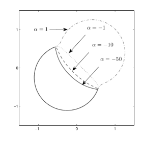
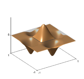
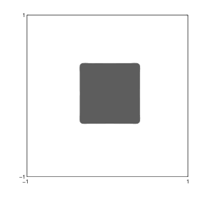
Clearly for $c>0$, $\mathscr{I}_{c}(\vartheta)$ represents the interior of the $c$-level set of $\vartheta$. Based on (43) and the smoothness of the bumps, we obviously have that as $c\rightarrow 0^{+}$, $\mathscr{I}\!\!_{c}(\psi_{j}+\psi_{k})$ would tend to $\mathscr{I}\!\!_{c}(\psi_{j})\bigcup\mathscr{I}\!\!_{c}(\psi_{k})$. More generally for $\alpha_{j}>0$, $\mathscr{I}\!\!_{c}(\sum_{j=1}^{m_{0}}\alpha_{j}\psi_{j})$ tends to $\bigcup_{j=1}^{m_{0}}\mathscr{I}\!\!_{c}(\psi_{j})$ as $(c/\alpha_{j})\rightarrow 0^{+}$. In other words, using relatively large CSRBF weights (as compared to $c$) can imply reconstruction of the shape through the union of a collection of floating balls of various radii. Moreover $\mathscr{I}\!\!_{c}(\psi_{j}-\alpha_{k}\psi_{k})$ would tend to $\mathscr{I}\!\!_{c}(\psi_{j})\!\setminus\!\mathscr{I}\!\!_{c}(\psi_{k})$ as $c\rightarrow 0^{+}$ and $\alpha_{k}\rightarrow+\infty$. In a more general fashion, $\mathscr{I}\!\!_{c}(\alpha_{j}\psi_{j}-\alpha_{k}\psi_{k})$ tends to $\mathscr{I}\!\!_{c}(\psi_{j})\!\setminus\!\mathscr{I}\!\!_{c}(\psi_{k})$ as $(c/\alpha_{j})\rightarrow 0^{+}$ and $(\alpha_{k}/\alpha_{j})\rightarrow+\infty$. Therefore in this context, bumps with larger negative coefficients can yield holes or inflect the shape by excluding some portions of it. We would consider the two aforementioned properties of the CSRBFs as a “pseudo-logical” behavior of these functions. This property can result in rather high curvature geometries with a limited number of bumps. Besides high curvature regions, low curvature segments (e.g., an almost straight line in $\mathbb{R}^{2}$ or a planar segment in $\mathbb{R}^{3}$) can be formed by interaction of two identical bumps but with opposite signs at their footprint intersections. Figure 1.a sheds more light on aforementioned facts, and shows the interaction of two bumps, which for instance can represent a crescent with two rather sharp corners ($\alpha=-50$), or a contour with a low curvature segment ($\alpha=-1$). As a second example, a representation of a square using only 5 bumps is depicted in Figures 1.b and 1.c.

Figure 1: (a) Left: A close to zero ($c=0.01$) level set of the function $\psi_{1}+\alpha\psi_{2}$ for various values of $\alpha$. The CSRBF used is the Wendland’s function $\psi_{1,1}$ (cf. Table 1), the dilation factors are $\beta_{1}=\beta_{2}=1$ and the centers are taken as $\chi_{1}=(-\frac{1}{4},-\frac{1}{4})$ and $\chi_{2}=(\frac{2}{5},\frac{2}{5})$. (b) Center: A PaLS function involved in representation of a square at a close to zero level set. Only 5 bumps are involved. (c) Right: The representation of the square

The most commonly used CSRBFs are those called Wendland’s functions [81]. The smoothness and the compact support provided by Wendland’s functions are of interest and hence we shall use them as the basis for our PaLS approach. Wendland’s functions follow the general form of

$$\psi_{n,l}(r)=\left\{\begin{array}[]{lr}P_{n,l}(r)&0\leq r\leq 1\\ 0&r>1\end{array}\right.$$ (45)

when representing an RBF in $\mathbb{R}^{n}$, with $P_{n,l}$ being a univariate polynomial of degree $\lfloor n/2\rfloor+3l+1$. In terms of smoothness, this class of RBFs belong to $C^{2l}$. A derivation of these functions is provided in [81], from which we have listed the first few functions in Table 1.

Table 1: Compactly supported RBFs of minimal degree where $\ell=\lfloor n/2\rfloor+l+1$ and $(1-r)_{+}=\max\{0,1-r\}$

Function	Smoothness
$\psi_{n,1}(r)=(1-r)_{+}^{\ell+1}((\ell+1)r+1)$	$C^{2}$
$\psi_{n,2}(r)=(1-r)_{+}^{\ell+2}((\ell^{2}+4\ell+3)r^{2}+(3\ell+6)r+3)$	$C^{4}$
$\psi_{n,3}(r)=(1-r)_{+}^{\ell+3}((\ell^{3}+9\ell^{2}+23\ell+15)r^{3}+$	$C^{6}$
$\hskip 56.9055pt(6\ell^{2}+36\ell+45)r^{2}+(15\ell+45)r+15)$

In the next section we discuss the regularized heaviside function and explain how choosing an appropriate version of this function in (23), can pave the path for exploiting the pseudo-logical behavior of the bumps.

5.3 Numerical Approximation of the Heaviside Function

In a shape-based representation such as (23), solving the inverse problem numerically and making the evolution of the level set function possible requires using a smooth version of the heaviside function. A possible $C^{\infty}$ regularization of $H(.)$ denoted as $H_{1,\epsilon}$ is the one used in [16], as

$$H_{1,\epsilon}(x)=\frac{1}{2}\big{(}1+\frac{2}{\pi}\arctan(\frac{\pi x}{\epsilon})\big{)}.$$ (46)

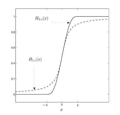
This function is commonly used in shape-based applications and specifically in the recent parametric representations of the level set function in image segmentation [29, 5]. Chan et al. in [14] have studied the characteristics of the resulting level set functions using $H_{1,\epsilon}$ as the evolution proceeds. In the context of the current shape-based problem for which $p_{i}(\mathbf{x})=\mathpzc{p}_{i}$ and $p_{o}(\mathbf{x})=\mathpzc{p}_{o}$, and considering the zero level set, (7) reveals that in an evolution process $\phi$ is likely to evolve towards a state that $H(\phi(\mathbf{x}))=1$ for $\mathbf{x}\in D$ and $H(\phi(\mathbf{x}))=0$ for $\mathbf{x}\in\Omega\setminus D$.

Figure 2: (a) Left: Two regularized versions of the heaviside function. (b) Right: Corresponding regularized delta functions

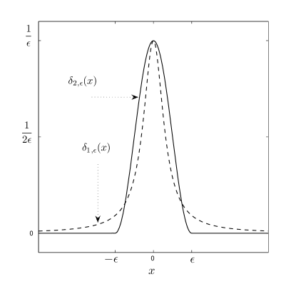Referring to Figure 2.a, one observes that when $H_{1,\epsilon}$ is used as the regularized heaviside function, in order to have $H_{1,\epsilon}(\phi)\simeq 1$ in $D$, the level set function should take rather large positive values (as compared to $\epsilon$) in this region. Analogously in $\Omega\setminus D$, $\phi$ is pushed to take rather large negative values. These constraints are implicitly imposed on the resulting level set function and specifically using CSRBFs in a PaLS approach as (37), the bumps are expected to distribute throughout $\Omega$ to form a level set function which takes rather large positive (or negative) values inside (or outside) $D$.

An alternative choice of the regularized Heaviside function is the $C^{2}$ function,

$$H_{2,\epsilon}(x)=\left\{\begin{array}[]{cl}1&x>\epsilon\\ 0&x<-\epsilon\\ \frac{1}{2}+\frac{x}{2\epsilon}+\frac{1}{2\pi}\sin(\frac{\pi x}{\epsilon})&|x|\leq\epsilon,\\ \end{array}\right.$$ (47)

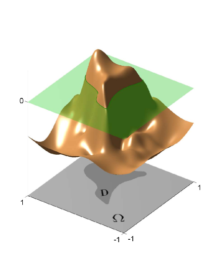
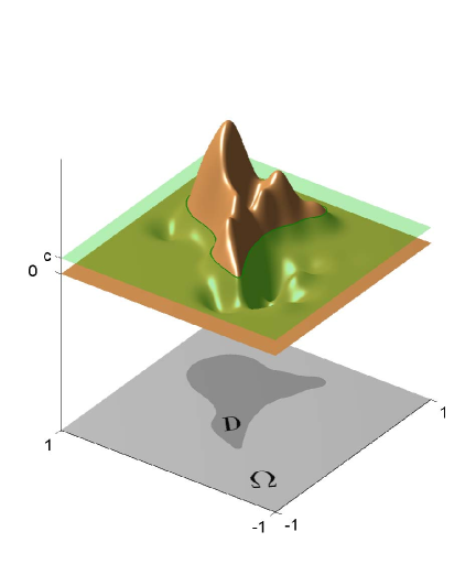
as proposed in [84]. It can be shown that if the nonzero level set $c$ and $\epsilon$ are appropriately set, using $H_{2,\epsilon}$ enables us to exploit the pseudo-logical behavior described previously. More specifically, for $c>0$, and $\phi$ being a weighted sum of some bumps, and therefore compactly supported itself, we clearly want the points for which $\phi\leq 0$ to belong to $\Omega\setminus D$, i.e., to correspond to the intensity $\mathpzc{p}_{o}$. Using (23), this requires having $H(\phi-c)=0$ for $\phi\leq 0$. Referring to Figure 2.a, this condition is satisfied when $H_{2,\epsilon}$ is chosen as the regularized heaviside function and $-c\leq-\epsilon$ (or in general case $|c|\geq\epsilon$ as the required criteria). Practically, this use of $H_{2,\epsilon}$ takes away the implicit constraint imposed on the level set function using $H_{1,\epsilon}$, i.e., the bumps do not have to spread throughout $\Omega$ and may only concentrate inside and about the shape $D$ to perform a higher resolution shaping. Figure 3 shows a typical shape representation resulted using $H_{1,\epsilon}$ and $H_{2,\epsilon}$ highlighting the pseudo-logical property.

Figure 3: (a) Left: A typical PaLS function resulted using $H_{1,\epsilon}$ with 65 bumps and considering the zero level set. (b) Right: A typical PaLS function resulted using $H_{2,\epsilon}$ with 30 bumps and considering the $c$ level set

Besides exploiting the pseudo-logical behavior, using $H_{2,\epsilon}$ can provide another advantage which reduces the dimensionality of the problem at every iteration, i.e., at every step of the evolution process, the cost function will be sensitive to a specific group of PaLS parameters. To further describe this behavior, consider the term $\delta_{rg}(\phi-c)\frac{\partial\phi}{\partial\mu_{j}}$ appearing in both the Jacobian and the approximate Hessian of $\mathscr{F}$ in (27) and (32). Also for an evolution iteration, assume the superscript $(t)$ indicating the value of every quantity at that iteration. If for a PaLS parameter such as $\mu\!_{j_{{}_{0}}}$

$$\delta_{rg}(\phi^{(t)}-c)\frac{\partial\phi^{(t)}}{\partial\mu\!_{j_{{}_{0}}}}\Big{|}_{\mu\!_{j_{{}_{0}}}=\mu\!_{j_{{}_{0}}}^{(t)}}=0\qquad\forall\mathbf{x}\in\Omega,$$ (48)

then using either one of the minimization schemes as (28) or (33) yields

$$\mu\!_{j_{{}_{0}}}^{(t+1)}=\mu\!_{j_{{}_{0}}}^{(t)}.$$ (49)

The reason for this result is clear for the gradient descent scheme (28), based on the fact that using (48) in (27) causes the $j_{{}_{0}}^{th}$ element of gradient vector to vanish and hence $\mu\!_{j_{{}_{0}}}^{(t)}$ remaining unchanged at the corresponding iteration. For the Levenberg-Marquardt scheme (33), using (48) in (32) causes all the elements in the $j_{{}_{0}}^{th}$ row of the approximate Hessian matrix to vanish, which results the corresponding equation

$$\lambda(\mu\!_{j_{{}_{0}}}^{(t+1)}-\mu\!_{j_{{}_{0}}}^{(t)})=0,$$ (50)

again equivalent to (49). Therefore, for either one of the minimization schemes, if (48) holds, the PaLS parameter $\mu\!_{j_{{}_{0}}}$ will stay unchanged in that iteration. We here describe a common case that (48) holds during the evolution process:

By using $H_{2,\epsilon}$ as the regularized level set function, the corresponding regularized delta function $\delta_{2,\epsilon}$ will be compactly supported (as shown in Figure 2.b), hence $\delta_{2,\epsilon}(\phi-c)$ is only nonzero for $c-\epsilon<\phi<c+\epsilon$. On the other hand, based on the PaLS approach presented in this paper using CSRBFs, for $\mu_{j}$ being any of the PaLS parameters $\alpha_{j}$, $\beta_{j}$ or $\chi_{j}^{(k)}$ corresponding to the bump $\psi_{j}$, we have

$$\operatorname{supp}(\frac{\partial\phi}{\partial\mu_{j}})\subseteq\operatorname{supp}(\psi_{j}).$$ (51)

This fact is easily observable in (39), (40) and (41), where the related derivatives can only have nonzero values in $\operatorname{supp}(\psi_{j})$. Therefore, if at some iteration and for a bump $\psi_{j_{{}_{0}}}$,

$$\operatorname{supp}\big{(}\delta_{2,\epsilon}(\phi-c)\big{)}\cap\operatorname{supp}(\psi_{j_{{}_{0}}})=\emptyset,$$ (52)

then in that iteration we have

$$\delta_{2,\epsilon}(\phi-c)\frac{\partial\phi}{\partial\mu\!_{j_{{}_{0}}}}=0$$ (53)

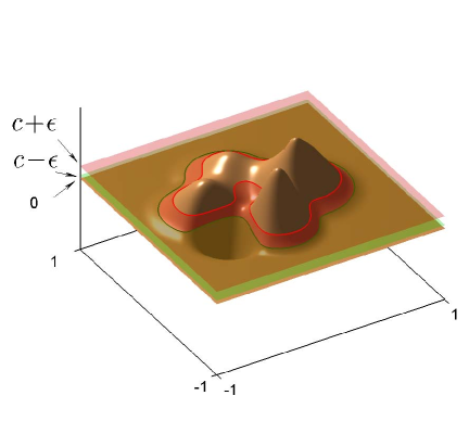
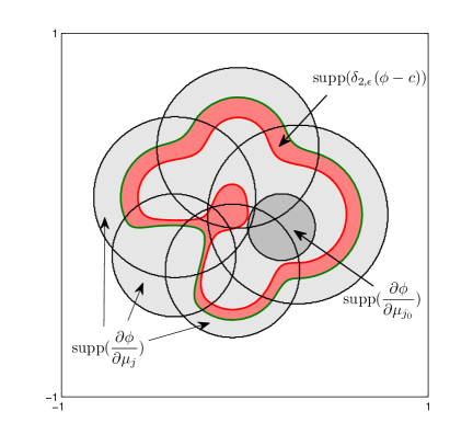
and therefore the PaLS parameters corresponding to $\psi_{j_{{}_{0}}}$ will stay unchanged in that iteration. Figure 4 illustrates this phenomenon, showing a PaLS function composed of 6 bumps at some iterations. For 5 of the bumps used, the corresponding support does intersect the region $\operatorname{supp}(\delta_{2,\epsilon}(\phi-c))$, and therefore their corresponding parameters have the potential to change at this state of the PaLS function. However, a bump denoted as $\psi_{j_{{}_{0}}}$, does not intersect $\operatorname{supp}\big{(}\delta_{2,\epsilon}(\phi-c))$, and the underlying PaLS parameters do not need to be considered in that iteration. This approach is similar to the narrow-banding approach in traditional level-set methods [2, 66, 59], where the values of the level set function are only updated on a narrow band around the zero level set and hence reducing the computation load. In our approach, however, this band is the points for which $c-\epsilon<\phi<c+\epsilon$ and the bumps which do not intersect with this band do not evolve at the corresponding iteration and hence their corresponding parameters are not updated.

Figure 4: (a) Left: A typical PaLS function composed of 6 bumps, and the $c\pm\epsilon$ level sets.                           (b) Right: The bumps with active evolving parameters and the frozen bump

In the next section, through a number of examples drawn from a wide range of applications, we will show the superior performance of the proposed method specifically exploiting the pseudo-logical behavior of the CSRBFs.

6 Examples

In this section, we examine our proposed method for three different inverse problems, namely electrical resistance tomography, X-ray computed tomography and diffuse optical tomography. The examples are simulated for 2D imaging and the results are provided in each section. Throughout all the examples, $\Omega$ denotes the region to be imaged and $D$ denotes the shape domain as stated in the previous sections.

6.1 Electrical Resistance Tomography

As the first example we consider electrical resistance tomography (ERT) categorized as a severely ill-posed problem [31, 22]. The objective of this problem is the reconstruction of the electrical conductivity within a region of interest based on the potential or current measurements performed at the periphery of that region. Such reconstructions may be applicable in various areas such as medical imaging [17], geophysics [23] and environmental monitoring [19].

For many geophysical applications the underlying physical model describing the DC potential $u(\mathbf{x})$ inside $\Omega$ in terms of the conductivity $\sigma(\mathbf{x})$ and the current source distribution $s(\mathbf{x})$ is

$$\nabla\cdot\big{(}\sigma(\mathbf{x})\nabla u(\mathbf{x})\big{)}=s(\mathbf{x})\quad\;\;\mbox{in}\;\;\Omega,$$ (54)

$$\sigma\frac{\partial u}{\partial\nu}=0\qquad\quad\quad\quad\qquad\quad\mbox{on}\;\;\partial\Omega_{n}\subset\partial\Omega,$$

$$u=0\;\;\qquad\quad\quad\quad\qquad\quad\quad\mbox{on}\;\;\partial\Omega_{d}=\partial\Omega\setminus\partial\Omega_{n},$$

where $\nu$ denotes the outward unit normal on $\partial\Omega$ and $\partial\Omega_{n}$ and $\partial\Omega_{d}$ correspond to Neumann and Dirichlet boundaries. In many of the applications (e.g., see [65, 45, 75, 54]) the Dirichlet boundary condition is imposed as an approximation to the potential in regions far from the actual imaging region, and is used here for simplicity. For arbitrary distributions of the conductivity, (54) is usually solved numerically by means of finite element or finite difference methods [69, 83]. However, as the main focus of the paper, we concentrate on piecewise constant conductivity distribution as $\sigma(\mathbf{x})=\sigma_{i}$ for $\mathbf{x}\in D$ and $\sigma(\mathbf{x})=\sigma_{o}$ for $\mathbf{x}\in\Omega\setminus D$.

For the inverse problem, the sensitivities of the measurements to perturbations of the conductivity (in our approach the perturbations of the PaLS parameters) are required. For $s(\mathbf{x})=\delta(\mathbf{x}-\mathbf{x}_{s})$, i.e., a point source current at $\mathbf{x}_{s}\in\Omega$, we denote by $u_{s}(\mathbf{x})$ the resulting potential over the domain $\Omega$ and consider the measured potential at $\mathbf{x}_{d}\in\Omega$ as

$$u_{ds}=\int_{\Omega}u_{s}(\mathbf{x})\delta(\mathbf{x}-\mathbf{x}_{d})\mbox{d}\mathbf{x}.$$ (55)

The variation of $u_{ds}$ resulting from a perturbation $\delta\sigma$ in the conductivity (i.e., the Fréchet derivative of the measurements with respect to the conductivity) can be then expressed as [62, 68]

$$\frac{\mbox{d}u_{ds}}{\mbox{d}\sigma}\;[\delta\sigma]=\int_{\Omega}\delta\sigma\;\nabla u_{s}\cdot\nabla u_{d}\;\mbox{d}\mathbf{x},$$ (56)

where $u_{d}$ is the adjoint field that results from placing the current point source at $\mathbf{x}_{d}$. To express the inverse problem in a PaLS framework, we consider $\mathcal{M(.)}$ as the nonlinear forward model mapping the conductivity distribution into a vector of voltage measurements $\mathbf{u}$ obtained by performing $M$ experiments, having a different point source position at each experiment and making $N_{\ell}$ potential measurements for $\ell=1,2,\cdots,M$. Having the residual operator $\mathcal{R}(\sigma)=\mathcal{M}(\sigma)-\mathbf{u}$ and using (56), the Fréchet derivative denoted as $\mathcal{R}^{\prime}(\sigma)[.]$ can be considered as a vector consisting of $M$ sub-vectors $\mathcal{R}^{\prime}_{\ell}(\sigma)[.]$, structured as

$$\mathcal{R}^{\prime}_{\ell}(\sigma)[\delta\sigma]=\left(\begin{array}[]{c}\int_{\Omega}\delta\sigma\;\nabla u_{\ell}\cdot\nabla u_{1}^{\ell}\;\mbox{d}\mathbf{x}\\ \vdots\\ \int_{\Omega}\delta\sigma\;\nabla u_{\ell}\cdot\nabla u_{N_{\ell}}^{\ell}\;\mbox{d}\mathbf{x}\end{array}\right).$$ (57)

Here $u_{\ell}$ denotes the potential in the $\ell^{\mbox{th}}$ experiment and $u_{i}^{\ell}$ denotes the adjoint field corresponding to the $\ell^{\mbox{th}}$ experiment resulted from placing the current point source at the $i^{\mbox{th}}$ measurement point. Having $\mathcal{R}^{\prime}(\sigma)[.]$ in hand, one can obtain the PaLS evolution through using (4) and (32) in (33).

Figure 5: (a) Left: The 2D modelling region for ERT. The darker interior region is the imaging region surrounded by the sources and detectors. The dashed lines correspond to dipole nodes used in every experiment (b) Right: The gray region shows the shape to be reconstructed in the ERT problem. The dots with “+” and “-” signs correspond to the centers of positive and negative weighted bumps in the initial state of the problem. The black contour is the resulting $c$-level set of the initial PaLS function.

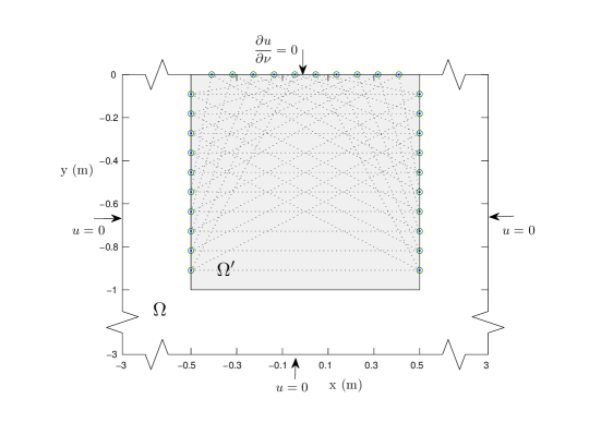
For the purpose of this example, we model the electric potential within the box $\Omega=[-3,3]\times[-3,0]$ all dimensions in units of meters in $x-y$ plane. Here $\partial\Omega_{n}$ corresponds to the top surface ($y=0$) and $\partial\Omega_{d}$ corresponds to the sides and bottom boundaries as shown in Figure 5.a. The region to be imaged is the square $\Omega^{\prime}=[-0.5,0.5]\times[-1,0]$, where 30 points are allocated to the sensors placed equally spaced on the top and the sides of this region (shown as small circles in the figure). A total of $M=40$ experiments are performed and in every experiment two of the sensors are used as a current dipole (superposition of two point sources with opposite signs) and the remaining 28 sensors measure the potential at the corresponding positions. The dipole sources are chosen in a cross-medium configuration, where the electrodes corresponding to every experiment are connected with a dashed line as again shown in Figure 5.a. With this configuration we try to enforce electric current flow across the medium anomalies and obtain data sets more sensitive to shape characteristics. For the simulation, we use the finite difference method where $\Omega$ is discretized to 125 grid points in the $x$ direction and 100 points in the $y$ direction. The gridding is performed in a way that we have a uniform $75\times 75$ grid within $\Omega^{\prime}$ (excluding the boundaries containing the sensors) and the exterior grids linearly get coarser as they get further from $\Omega^{\prime}$ in the $x$ and $y$ direction. The forward modelling is performed over the whole collection of grids in $\Omega$, while the inversion only involves the pixels within $\Omega^{\prime}$ (known as active cells [60]).

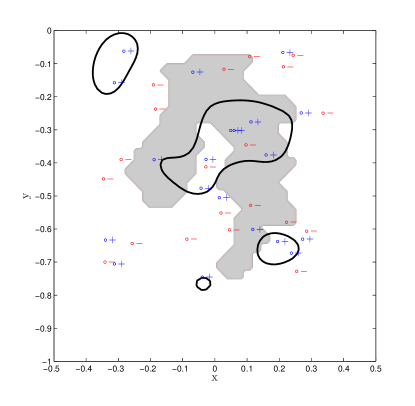
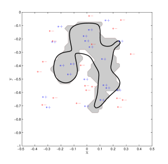
The shape to be reconstructed is shown as the gray region in Figure 5.b. This shape is a threshholded version of a real scenario and is of particular interest here because it has a concavity facing the bottom where there are no measurements performed. The values for the anomaly conductivities are $\sigma_{i}=0.05\;\mbox{Sm}^{-1}$ and $\sigma_{o}=0.01\;\mbox{Sm}^{-1}$ and the conductivity value used for $\Omega\setminus\Omega^{\prime}$ is the same as the true value of $\sigma_{o}$ in all our inversions. In the inversions we consider the data $\mathbf{u}$ to be the measured potentials generated by the true anomaly with $1\%$ additive Gaussian noise. For the shape representation we use $H_{2,\epsilon}$ with $\epsilon=0.1$ and we consider the $c=0.15$ level set.

For the PaLS representation (36) we have $m_{0}=40$ terms and the Wendland’s function $\psi_{1,1}$ is used as the corresponding bump. For the initial PaLS parameters, we consider a random initial distribution of the centers $\boldsymbol{\chi}_{j}$, within the square $[-0.4,0.4]\times[-0.8,0]$. The weighting coefficients are initialized as $\alpha_{j}=\pm 0.2$ where the centers of alternatively positive and negative weighted bumps are shown with $``+"$ and $``-"$ signs in Figure 5.b. The positive initial values of $\alpha_{j}$ are taken slightly bigger than $c$ to have some initial $c$-level sets. The purpose behind having alternative bump signs is to have the narrow-band $\operatorname{supp}(\delta_{2,\epsilon}(\phi-c))$ cover various regions of $\Omega^{\prime}$ and increase the chance of initially involving more bumps in the shaping as explained in previous section and Figure 4. The dilation factors are taken uniformly to be $\beta_{j}=4$, as an initialization to make the support radii of the bumps small enough for capturing details and more or less large enough to carpet the region $\Omega^{\prime}$. Our intention for this initialization of the PaLS parameters is to provide a rather simple, reproducible and general initialization. The stopping criteria in the reconstructions is when the norm of the residual operator reaches the noise norm (known in the regularization literature as the discrepancy principle [77]).

Figure 6: (a) Left: The result of reconstructing the shape using PaLS approach after 26 iterations, the centers $\boldsymbol{\chi}_{j}$ and their corresponding weight signs are shown. (b) Center: Result of using the traditional level set method after 39 iterations (c) Right: The result of reconstructing both the shape and the binary conductivity values after 32 iterations

Figure 7: (a) Left: The initial PaLS function (b) Right: The final PaLS function for the shape-only reconstruction of Figure 6.a

Figure 8: Residual error reduction through the iterative process for the shape only reconstruction, using PaLS approach and the traditional level set method

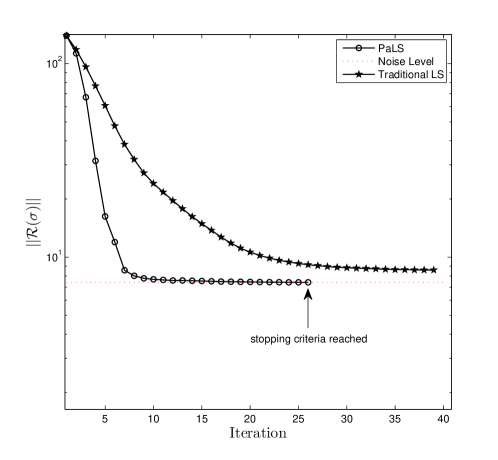
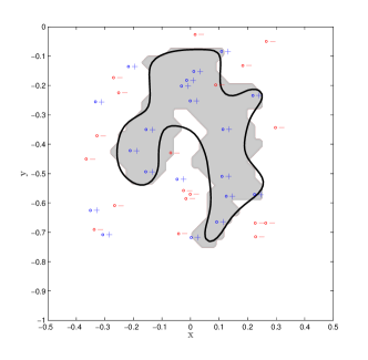
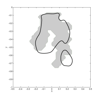
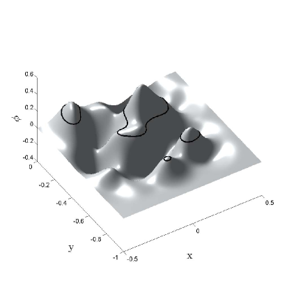
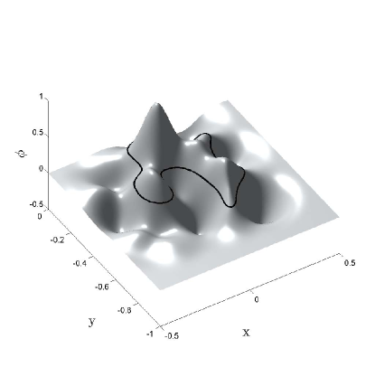
Figure 6.a shows the shape reconstruction using the PaLS approach, and assuming the values $\sigma_{i}$ and $\sigma_{o}$ are a priori known. Figure 6.b shows the result of the same problem using a typical Gauss-Newton approach with the level set function defined as a signed distance function over the pixels and a smoothing regularization added as explained in [69]. This algorithm only considers shape reconstruction (i.e., $\sigma_{i}$ and $\sigma_{o}$ are considered known) and it is initialized with the same contour as the initial $c$-level set contour of the PaLS approach. As the results in Figure 6.a and 6.b show, the PaLS approach performs well in reconstructing major shape characteristics, while the traditional level set approach fails to provide a good reconstruction in low sensitivity regions close to the bottom and does not capture the concavity. Figure 6.c shows the result of reconstructing both the shape and the anomaly values using the PaLS approach, where this time the PaLS evolution takes slightly more iterations (32 iterations verses 26), but the resulting reconstruction still well represents the shape. The initial values used for the conductivity values are $\sigma_{i}^{(0)}=0.01\;\mbox{Sm}^{-1}$ and $\sigma_{o}^{(0)}=0.005\;\mbox{Sm}^{-1}$ and the final resulting values are $\sigma_{i}^{(32)}=0.056\;\mbox{Sm}^{-1}$ and $\sigma_{o}^{(32)}=0.010\;\mbox{Sm}^{-1}$, which show a good match with the real values. To illustrate the behavior of the PaLS function, in Figure 7 we have shown the initial and final PaLS functions for the shape only reconstruction. Also to compare the convergence behaviors of the PaLS approach and the traditional level set approach, in Figure 8 we show the residual error through the evolution steps for both methods. Using the PaLS approach the stopping criteria is met after 26 iterations while traditional level set method reaches a local minima after 39 iterations (the updates after 39 iterations become so small that it stops evolving further).

6.2 X-ray Computed Tomography

As the second example and a mildly ill-posed problem, we consider X-ray Computed Tomography (CT) [20]. In this imaging technique, X-ray photons are transmitted through the object of interest and the intensity of transmitted ray is measured at the boundaries to reconstruct the object’s attenuation coefficient. The contrast between the attenuation characteristics of different materials can provide structural information about the object being imaged. X-ray CT is among the most well known methods for imaging the body tissue in medical applications [35].

For an X-ray beam transmitting along a line $\mathcal{L}_{k}$ in the tissue, the photon intensity $\mathcal{X}_{k}$ measured at the detector side of the line can be written as

$$\mathcal{X}_{k}=\int I_{k}(\mathcal{E})\exp\big{(}-\int_{\mathcal{L}_{k}}\alpha(\mathbf{x},\mathcal{E})\;\mbox{d}\mathbf{x}\big{)}\;\;\mbox{d}\mathcal{E}$$ (58)

where $\alpha(\mathbf{x},\mathcal{E})$ denotes the attenuation coefficient, in general as a function of the position $\mathbf{x}$ and the energy of the incident ray $\mathcal{E}$, and $I_{k}(\mathcal{E})$ denotes the incident ray energy spectrum. In case of a monoenergetic beam as $I_{k}(\mathcal{E})=I_{0,k}\delta(\mathcal{E}-\mathcal{E}_{0})$, a measured quantity related to the photon intensity may be defined as

$$u_{k}:=-\log(\frac{\mathcal{X}_{k}}{I_{0,k}})=\int_{\mathcal{L}_{k}}\alpha(\mathbf{x})\mbox{d}\mathbf{x}.$$ (59)

Equation (59) simply relates the measurements to the Radon transform of the attenuation coefficient $\alpha(\mathbf{x})$ in a monoenergetic scenario. The quantities $u_{k}$ are actually what is considered as the data in CT imaging.

The Fréchet derivative of the CT measurements with respect to the attenuation coefficient is expressed as

$$\frac{\mbox{d}u_{k}}{\mbox{d}\alpha}\;[\delta\alpha]=\int_{\mathcal{L}_{k}}\delta\alpha\;\mbox{d}\mathbf{x}.$$ (60)

Considering $\mathbf{u}$ to be the set of CT data collected along different paths $\mathcal{L}_{k}$, for $k=1,2,\cdots N$, and $\mathcal{M}(\alpha)$ as the forward model mapping the attenuation to the CT data set, based on (60) the sensitivity of the residual operator $\mathcal{R}(\alpha)=\mathcal{M}(\alpha)-\mathbf{u}$ with respect to a perturbation in $\alpha$ can be written as

$$\mathcal{R}^{\prime}(\alpha)[\delta\alpha]=\left(\begin{array}[]{c}\int_{\mathcal{L}_{1}}\delta\alpha\;\mbox{d}\mathbf{x}\\ \vdots\\ \int_{\mathcal{L}_{N}}\delta\alpha\;\mbox{d}\mathbf{x}\\ \end{array}\right),$$ (61)

which we need for the PALS evolution process.

Figure 9: (a) Left: The 2D X-ray CT imaging setup (b) Right: The gray region shows the attenuation shape to be reconstructed. The dots with “+” and “-” signs correspond to the centers of positive and negative weighted bumps in the initial state of the problem. The black contour is the resulting $c$-level set of the initial PaLS function

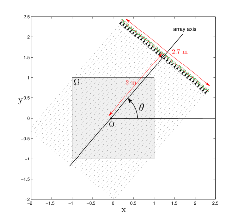
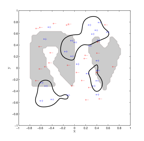
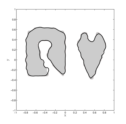
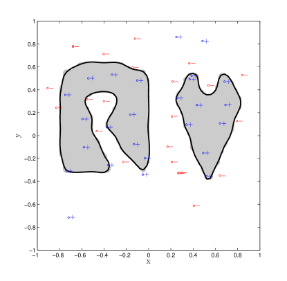
We consider 2D imaging over a square of $2\;\mbox{m}\times 2\;\mbox{m}$, i.e., $\Omega=[-1,1]\times[-1,1]$ in the $x-y$ plane, as shown in Figure 9.a. The region outside $\Omega$ is assumed to have zero attenuation. The X-ray beams are emitted as parallel beams and the measurements are performed through an equally spaced linear array of 34 sensors, the vertical axis of which makes an angle $\theta$ with the $x$ axis. For a full view X-ray CT we have $\theta_{0}\leq\theta\leq\theta_{0}+\pi$, while in a limited view scenario, and hence a more ill-posed problem, $\theta$ varies in a smaller angular domain. The shape to be reconstructed is shown in Figure 9.b, which is brought here from [72] as a rather complex shape to examine the flexibility of the PaLS approach. The region $\Omega$ is discretized into $64\times 64$ uniform grid. The binary attenuation values are $\alpha_{i}=2.5\;\mbox{cm}^{-1}$ and $\alpha_{o}=1\;\mbox{cm}^{-1}$. For the purpose of imaging, the forward model measurements are performed at every $1$ degree angle. For the PaLS representation, we use $m_{0}=50$ bumps with the centers $\boldsymbol{\chi}_{j}$, distributed randomly as shown in Figure 9.b. For this example we use slightly more bumps due to the better posed nature of the problem (at least in the full view case) and the more complex shape. Again to roughly carpet the domain $\Omega$ with the bumps we uniformly take the dilation factors to be $\beta_{j}=2.5$. The other PaLS settings used are similar to those of the ERT example in the previous section.

Figure 10: (a) Left: The result of reconstructing both the shape and the anomaly values in a $5\%$ noise case using the PaLS approach, convergence achieved after 20 iterations (b) Right: Result of using the same data set with traditional level set method to recover shape only, assuming attenuation coefficients are known, convergence achieved after 14 iterations

Figure 11: (a) Left: The result of PaLS shape reconstruction in a $1\%$ noise case to show the flexibility of following shape details due to the pseudo-logical property, convergence achieved after 42 iterations (b) Right: The corresponding PaLS function

Figure 12: (a) Left: The PaLS shape reconstruction in a limited view X-ray CT, convergence achieved after 49 iterations (b) Right: The performance of the traditional level set method for the same data set, reaching a local minima after 32 iterations

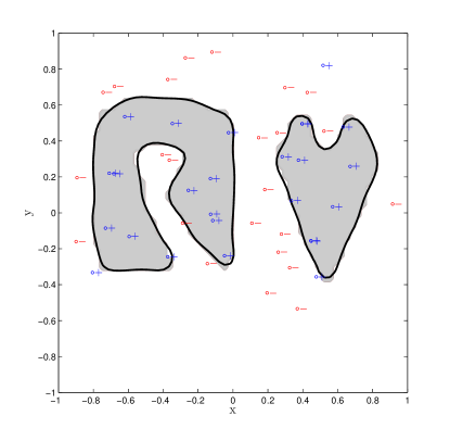
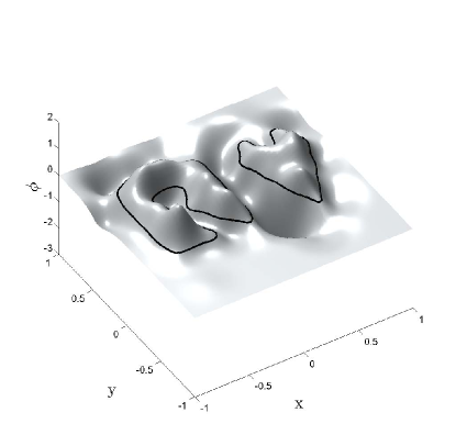
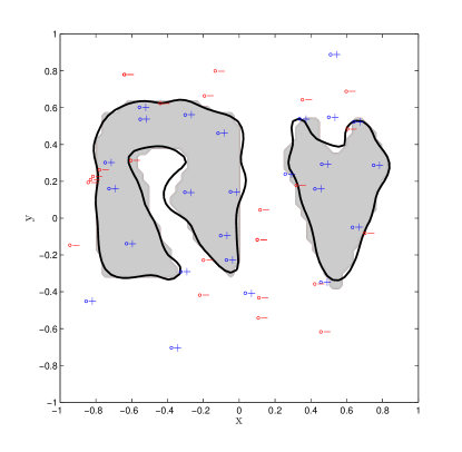
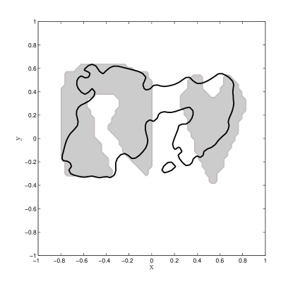
Figure 10.a shows the result of reconstructing both the shape and the attenuation values for a full view experiment where $0<\theta<\pi$. The synthetic data are obtained from the true attenuation map and by adding $5\%$ Gaussian noise to the measurements. The initial values used for the attenuations are $\alpha_{i}^{(0)}=1.5\;\mbox{cm}^{-1}$ and $\alpha_{o}^{(0)}=0.5\;\mbox{cm}^{-1}$ and the discrepancy principle stopping criteria is met after 20 iterations resulting the corresponding shape and the final values of $\alpha_{i}^{(20)}=2.494\;\mbox{cm}^{-1}$ and $\alpha_{o}^{(20)}=0.997\;\mbox{cm}^{-1}$, which are very well matched with the real quantities. We should mention here that when the attenuation values are assumed to be known, the number of iterations for shape reconstruction is only 12. The same data set is used to reconstruct the shape only, using the traditional level set method used in the ERT example and initialized with the same contour as the $c$-level set contour shown in Figure 9.b. The result of this reconstruction is shown in Figure 10.b. Due to the better posed nature of this problem, the pixel based level set method also provides a successful reconstruction for the geometry only. Note, however that the PaLS approach is solving a more challenging problem (i.e., reconstructing the attenuation values as well as the shape), thanks to the pseudo-logical behavior of the bumps, the resulting shape follows the same detail levels as a pixel based level set function. This shaping capability of the PaLS is more highlighted when we use a less noisy data ($1\%$ Gaussian noise). The result is shown in Figure 11 where the convergence is achieved after 42 iterations, and the resulting contours follows the true shape in high level of details. Finally as a more challenging and very ill-posed problem, we now consider a limited view scenario where the angular domain is limited to $\pi/4<\theta<3\pi/4$, and fewer rays cross the anomalies. Two percent additive Gaussian noise is added to the synthetic data obtained from the true attenuation map. With the same problem setting as the full view case, Figure 12.a shows the result of reconstructing the shape using the PaLS approach. However, as shown in Figure 12.b, the traditional level set method applied to this problem given the attenuation values, fails to provide a complete reconstruction and stops further shape enhancement after reaching a local minima.

6.3 Diffuse Optical Tomography

As the third application we consider diffuse optical tomography (DOT). In this imaging method data are obtained by transmitting near-infrared light into a highly absorbing and scattering medium and then recording the transmitted light. As the inverse problem of interest the photon flux is measured on the surface to recover the optical properties of the medium such as absorption and/or reduced scattering functions. A well known application of this method is breast tissue imaging, where the differences in the absorption and scattering may indicate the presence of a tumor or other anomaly [7]. For given absorption and scattering functions a number of mathematical models have been proposed in the literature to determine the synthetic data (photon flux) [3]. We focus on the frequency-domain diffusion model in which the data is a non-linear function of the absorption and scattering functions.

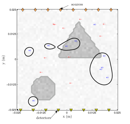
Consider $\Omega$, a square with a limited number of sources on the top and a limited number of detectors on either the top or bottom or both. We use the diffusion model in [3] modified for the 2D case where the photon flux $u(\mathbf{x};\omega)$ is related to input $s(\mathbf{x};\omega)$ through

$$-\nabla\cdot\beta(\mathbf{x})\nabla u(\mathbf{x};\omega)+\alpha(\mathbf{x})u(\mathbf{x};\omega)+i\frac{\omega}{v}u(\mathbf{x};\omega)=s(\mathbf{x};\omega),$$ (62)

with the Robin boundary conditions

$$u(\mathbf{x};\omega)+2\beta(\mathbf{x})\frac{\partial u(\mathbf{x};\omega)}{\partial\nu}=0,\qquad\mathbf{x}\in\partial\Omega.$$ (63)

Here, $\beta(\mathbf{x})$ denotes the diffusion, which is related to the reduced scattering function $\mu_{s}^{\prime}(\mathbf{x})$, by $\beta(\mathbf{x})=1/\big{(}3\mu_{s}^{\prime}(\mathbf{x})\big{)}$, $\alpha(\mathbf{x})$ denotes absorption and $\partial/\partial\nu$ denotes the normal derivative. We also have $i=\sqrt{-1}$, $\omega$ as the frequency modulation of light and $v$ being the speed of light in the medium. Knowing the source and the functions $\alpha(\mathbf{x})$ and $\beta(\mathbf{x})$, we can compute the corresponding $u(\mathbf{x};\omega)$ everywhere, in particular, at the detectors.

As the inverse problem, we consider a case that the reduced scattering function is known and we want to reconstruct the absorption $\alpha(\mathbf{x})$ from the data. Again for this problem we consider a point source $s(\mathbf{x};\omega)=\delta(\mathbf{x}-\mathbf{x}_{s})$ for $\mathbf{x}_{s}\in\partial\Omega$, which results in a photo flux $u_{s}(\mathbf{x};\omega)$ in $\Omega$. For a measurement at $\mathbf{x}_{d}\in\Omega$ as

$$u_{ds}=\int_{\Omega}u_{s}(\mathbf{x};\omega)\delta(\mathbf{x}-\mathbf{x}_{d})\mbox{d}\mathbf{x},$$ (64)

the variations with respect to the variations in the absorption can be written as [3]

$$\frac{\mbox{d}u_{ds}}{\mbox{d}\alpha}[\delta\alpha]=\int_{\Omega}\delta\alpha\;u_{s}(\mathbf{x};\omega)\;u_{d}(\mathbf{x};\omega)\mbox{d}\mathbf{x},$$ (65)

with $u_{d}$ being the adjoint field caused by having the point source at $\mathbf{x}_{d}$. Identical to the notation used for the ERT problem, consider $\mathcal{R}(\alpha)=\mathcal{M}(\alpha)-\mathbf{u}$ as the residual operator where the data vector $\mathbf{u}$ contains the measurements of $N_{\ell}$ detectors from $M$ experiments. Based on (65) the $\ell^{\mbox{th}}$ block of $\mathcal{R}^{\prime}(\alpha)[.]$ corresponding to the $\ell^{\mbox{th}}$ experiment is

$$\mathcal{R}^{\prime}_{\ell}(\alpha)[\delta\alpha]=\left(\begin{array}[]{c}\int_{\Omega}\delta\alpha\;u_{\ell}\;u_{1}^{\ell}\;\mbox{d}\mathbf{x}\\ \vdots\\ \int_{\Omega}\delta\alpha\;u_{\ell}\;u_{N_{\ell}}^{\ell}\;\mbox{d}\mathbf{x}\end{array}\right),$$ (66)

with $u_{\ell}$ denoting the photon flux in the $\ell^{\mbox{th}}$ experiment and $u_{i}^{\ell}$ being the adjoint field.

Figure 13: The 2D DOT imaging setup with the sources and detectors setting. The gray region shows the absorption shape, while $2\%$ Gaussian noise is added to the absorption as a heterogeneity. The dots with “+” and “-” signs correspond to the centers of positive and negative weighted bumps in the initial state of the problem. The black contour is the resulting $c$-level set of the initial PaLS function

Figure 14: (a) Left: The PaLS shape-only reconstruction, stopping criteria achieved after 152 iterations in case $0.1\%$ data noise and $2\%$ heterogeneity (b) Right: The results of shape reconstruction in case of only heterogeneity in the absorption. The evolution is manually stopped after 200 iterations, showing the results

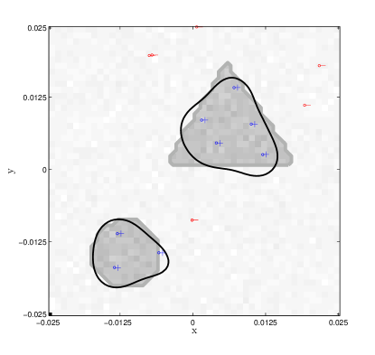
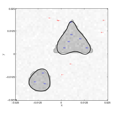
For the purpose of this example we consider a very ill-posed problem where $\Omega$ corresponds to a $5\mbox{cm}\times 5\mbox{cm}$ imaging region, and there are only 8 point sources on the top and 8 detectors at the bottom. In every experiment only one of the sources is on and the measurements are performed at the bottom detectors. We have $\mu_{s}^{\prime}(\mathbf{x})=6\;\mbox{cm}^{-1}$ throughout $\Omega$. The measurements are performed at DC mode, $25$ MHz and $50$ MHz. The absorption binary distribution is shown in Figure 13 with values $\alpha_{i}=0.015\;\mbox{cm}^{-1}$ and $\alpha_{o}=0.005\;\mbox{cm}^{-1}$. To make the problem more challenging we made the absorption distribution slightly heterogeneous by adding $2\%$ white Gaussian noise to it. For the PaLS setting, due to the very ill-posed nature of the problem we use relatively fewer bumps, i.e., $m_{0}=20$. Similar to the previous two examples the centers $\boldsymbol{\chi}_{j}$ corresponding to positive and negative weighted bumps are taken randomly inside $\Omega$ as shown in Figure 13. Again to have reasonable initial support radius for the bumps the dilation factors are set to be $\beta_{j}=80$. Other PaLS settings are similar to the previous examples. The forward model is solved using finite difference method by discretizing $\Omega$ to $50\times 50$ grid points. Figure 14.a shows the result of our shape-only reconstruction after 152 iterations, when the true absorption map is used to generate the data and $0.1\%$ Gaussian noise is added to it. In case of not having any noise in the data (but still considering the heterogeneity in the absorption), the results after 200 iterations are shown in figure 14.b. Although the current problem settings make it very ill-posed and extremely hard for shape reconstruction, the PaLS approach shows reasonable reconstructions, providing important details. For this very ill-posed problem, using the traditional level set method we failed to generate useful reconstructions.

7 Concluding Remarks

In this paper we proposed a parametric level set approach to shape based inverse problems. The basic formulation of the problem is kept general, emphasizing the fact that numerically, an appropriate parametrization of the level set function is capable of reducing the problem dimensionality and intrinsically regularizes the problem. Through such modelling the level set function is more likely to remain well behaved, and therefore there is no need to re-initialize as in traditional level set methods. Moreover, based on the fact that the number of underlying parameters in a parametric approach is usually much less than the number of pixels (voxels) resulting from the discretization of the level set function, we make a use of a Newton type method to solve the underlying optimization problem. We specifically considered using compactly supported radial basis functions, which used as proposed provides two main advantages besides being parametric; first, the pseudo-logical property allows for recovery of wide range of shapes; and second, implicit narrow-banding for the evolution.

Although in this paper, we only considered compactly supported radial basis functions as the bump functions with circular support, a combination of sufficiently smooth bumps with various types of supports may be considered in applications where there is more prior information about the shape and its general geometric structure. An efficient classification of such functions for various types of shapes and problems (i.e., forming a basis dictionary) would be a future direction of research. Although in the examples presented in this work the number of RBFs where coarsely chosen, we are currently developing some ideas to adoptively determine the number of basis elements using a sparse signal processing approach. Clearly this matter is beyond the scope of this paper and is planned to be presented as a future work. Moreover, for sake of simplicity in this paper we only considered 2D problems, whereas the efficiency of a parametric approach is more pronounced for 3D shape reconstructions where the contrast between the number of voxels and the number of PaLS parameters in a parametric approach is more significant. Efficiently modelling 3D scenarios via both parametric shape representation and appropriate texture and heterogeneity models is an important future direction and a continuation of the current work.

References

- [1] R. Acar and CR Vogel, Analysis of bounded variation penalty methods for ill-posed problems, Inverse problems, 10 (1994), pp. 1217–1229.
- [2] D. Adalsteinsson and J.A. Sethian, A fast level set method for propagating interfaces, Journal of Computational Physics, (1995).
- [3] SR Arridge, Optical tomography in medical imaging, Inverse problems, 15 (1999), pp. R41–R93.
- [4] M.S. Berger, Nonlinearity and functional analysis, (1977).
- [5] O. Bernard, D. Friboulet, P. Thévenaz, and M. Unser, Variational B-spline level-set: a linear filtering approach for fast deformable model evolution, IEEE Transactions on Image Processing, 18 (2009), pp. 1179–1191.
- [6] D.P. Bertsekas, Nonlinear Programming, Athena Scientific, Belmont, MA, 1999.
- [7] DA Boas, DH Brooks, EL Miller, CA DiMarzio, M. Kilmer, RJ Gaudette, and Q. Zhang, Imaging the body with diffuse optical tomography, IEEE Signal Processing Magazine, 18 (2001), pp. 57–75.
- [8] MD Buhmann, Radial basis functions, Acta numerica, 9 (2001), pp. 1–38.
- [9] M. Burger, A framework for the construction of level set methods for shape optimization and reconstruction, Interfaces and Free boundaries, 5 (2003), pp. 301–330.
- [10] , Levenberg-Marquardt level set methods for inverse obstacle problems, Inverse problems, 20 (2004), pp. 259–282.
- [11] M. Burger and S.J. Osher, A survey on level set methods for inverse problems and optimal design, European Journal of Applied Mathematics, 16 (2005), pp. 263–301.
- [12] J.T. Bushberg, J.A. Seibert, E.M. Leidholdt Jr, J.M. Boone, and E.J. Goldschmidt Jr, The essential physics of medical imaging, vol. 30, 2003.
- [13] J. Carrera, A. Alcolea, A. Medina, J. Hidalgo, and L.J. Slooten, Inverse problem in hydrogeology, Hydrogeology Journal, 13 (2005), pp. 206–222.
- [14] T.F. CHAN, S. ESEDOGLU, and M. NIKOLOVA, Algorithms for finding global minimizers of image segmentation and denoising models, SIAM journal on applied mathematics, 66 (2006), pp. 1632–1648.
- [15] T.F. Chan and X.C. Tai, Level set and total variation regularization for elliptic inverse problems with discontinuous coefficients, Journal of Computational Physics, 193 (2004), pp. 40–66.
- [16] T.F. Chan and L.A. Vese, Active contours without edges, IEEE Transactions on image processing, 10 (2001), pp. 266–277.
- [17] M. Cheney, D. Isaacson, and J.C. Newell, Electrical impedance tomography, SIAM review, 41 (1999), pp. 85–101.
- [18] D. Colton and A. Kirsch, A simple method for solving inverse scattering problems in the resonance region, Inverse problems, 12 (1996), pp. 383–393.
- [19] W. Daily and A.L. Ramirez, Electrical imaging of engineered hydraulic barriers, Geophysics, 65 (2000), pp. 83–94.
- [20] M.E. Davison, The ill-conditioned nature of the limited angle tomography problem, SIAM Journal on Applied Mathematics, 43 (1983), pp. 428–448.
- [21] J.E. Dennis and R.B. Schnabel, Numerical methods for unconstrained optimization and nonlinear equations, Society for Industrial Mathematics, 1996.
- [22] M. Di Cristo and L. Rondi, Examples of exponential instability for elliptic inverse problems, Arxiv preprint math/0303126, (2003).
- [23] KA Dines and RJ Lytle, Analysis of electrical conductivity imaging, Geophysics, 46 (1981), p. 1025.
- [24] O. Dorn and D. Lesselier, Level set methods for inverse scattering, Inverse Problems, 22 (2006), p. R67.
- [25] , Level set techniques for structural inversion in medical imaging, Deformable Models, (2007), pp. 61–90.
- [26] O. Dorn, E.L. Miller, and C.M. Rappaport, A shape reconstruction method for EM tomography, Inverse problems, 16 (2000), pp. 1119–1156.
- [27] H.W. Engl, M. Hanke, and A. Neubauer, Regularization of inverse problems, Kluwer Academic Pub, 1996.
- [28] H. Feng, W.C. Karl, and D. Castanon, A curve evolution approach to object-based tomographic reconstruction, IEEE Transactions on Image Processing, 12 (2003), pp. 44–57.
- [29] A. Gelas, O. Bernard, D. Friboulet, R. Prost, and V. INSA, Compactly supported radial basis functions based collocation method for level-set evolution in image segmentation, IEEE Transactions on Image Processing, 16 (2007), pp. 1873–1887.
- [30] G.H. Golub, P.C. Hansen, and D.P. O’Leary, Tikhonov regularization and total least squares, SIAM Journal on Matrix Analysis and Applications, 21 (2000), pp. 185–194.
- [31] P.C. Hansen, Rank-deficient and discrete ill-posed problems: numerical aspects of linear inversion, Society for Industrial Mathematics, 1998.
- [32] R.L. Hardy, Multiquadric equations of topography and other irregular surfaces, Journal of Geophysical Research, 76 (1971), pp. 1905–1915.
- [33] K. Ito, K. Kunisch, and Z. Li, Level-set function approach to an inverse interface problem, Inverse problems, 17 (2001), p. 1225.
- [34] A.I. James, W.D. Graham, K. Hatfield, PSC Rao, and M.D. Annable, Optimal Estimation of Residual Non–Aqueous Phase Liquid Saturations Using Partitioning Tracer Concentration Data, Water Resources Research, 33.
- [35] W.A. Kalender, X-ray computed tomography, Physics in medicine and biology, 51 (2006), p. R29.
- [36] E.J. Kansa, Multiquadrics–A scattered data approximation scheme with applications to computational fluid-dynamics–II solutions to parabolic, hyperbolic and elliptic partial differential equations, Computers & Mathematics with applications, 19 (1990), pp. 147–161.
- [37] M.E. Kilmer, E.L. Miller, A. Barbaro, and D. Boas, 3D shape-based imaging for diffuse optical tomography, Applied Optics, 42 (2003), pp. 3129–3144.
- [38] M. Kilmer, E. Miller, M. Enriquez, and D. Boas, Cortical constraint method for diffuse optical brain imaging, in Proceedings of SPIE, vol. 5559, 2004, p. 381.
- [39] A. Kirsch, The domain derivative and two applications in inverse scattering theory, Inverse Problems, 9 (1993), pp. 81–96.
- [40] , Characterization of the shape of a scattering obstacle using the spectral data of the far field operator, Inverse problems, 14 (1998), pp. 1489–1512.
- [41] R. Kress and W. Rundell, A quasi-Newton method in inverse obstacle scattering, Inverse Problems, 10 (1994), pp. 1145–1157.
- [42] , Inverse obstacle scattering using reduced data, SIAM Journal on Applied Mathematics, 59 (1998), pp. 442–454.
- [43] R. Kress and A. Zinn, On the numerical solution of the three-dimensional inverse obstacle scattering problem, Journal of Computational and Applied Mathematics, 42 (1992), pp. 49–61.
- [44] G. Kristensson, Inverse problems for acoustic waves using the penalised likelihood method, Inverse Problems, 2 (1986), pp. 461–479.
- [45] D.J. LaBrecque, M. Miletto, W. Daily, A. Ramirez, and E. Owen, The effects of noise on Occam’s inversion of resistivity tomography data, Geophysics, 61 (1996), pp. 538–548.
- [46] A. Litman, D. Lesselier, and F. Santosa, Reconstruction of a two-dimensional binary obstacle by controlled evolution of a level-set, Inverse Problems, 14 (1998), pp. 685–706.
- [47] G.R. Liu and X. Han, Computational inverse techniques in nondestructive evaluation, CRC, 2003.
- [48] AK Louis, Medical imaging: state of the art and future development, vol. 8, Institute of Physics Publishing, 1992.
- [49] R. Marklein, K. Mayer, R. Hannemann, T. Krylow, K. Balasubramanian, KJ Langenberg, and V. Schmitz, Linear and nonlinear inversion algorithms applied in nondestructive evaluation, Inverse Problems, 18 (2002), pp. 1733–1759.
- [50] B.H. Miled and EL Miller, A projection-based level-set approach for anomaly reconstruction, Inverse Problems, 23 (2007), pp. 2375–2400.
- [51] EL Miller, M. Kilmer, and C. Rappaport, A new shape-based method for object localization andcharacterization from scattered field data, IEEE Transactions on Geoscience and Remote Sensing, 38 (2000), pp. 1682–1696.
- [52] EL MILLER and AS WILLSKY, A multiscale, statistically based inversion scheme for linearized inverse scattering problems, IEEE transactions on geoscience and remote sensing, 34 (1996), pp. 346–357.
- [53] V.A. Morozov and M. Stessin, Regularization methods for ill-posed problems, crc press Boca Raton, FL:, 1993.
- [54] I.R. Mufti, FINITE-DIFFERENCE RESISTIVITY MODELING FOR ARBITRARILY SHAPED TWO-DIMENSIONAL STRUCTURES, Geophysics, 41 (1976), p. 62.
- [55] A. Novruzi and M. Pierre, Structure of shape derivatives, Journal of Evolution Equations, 2 (2002), pp. 365–382.
- [56] S. Osher and R.P. Fedkiw, Level set methods and dynamic implicit surfaces, Springer Verlag, 2003.
- [57] S. Osher and J.A. Sethian, Fronts propagating with curvature-dependent speed: algorithms based on Hamilton-Jacobi formulations, Journal of computational physics, 79 (1988), pp. 12–49.
- [58] W.K. Park and D. Lesselier, Reconstruction of thin electromagnetic inclusions by a level set method, Inverse Problems, 25 (2009), p. 085010.
- [59] D. Peng, B. Merriman, S. Osher, H. Zhao, and M. Kang, A PDE-Based Fast Local Level Set Method* 1, Journal of Computational Physics, 155 (1999), pp. 410–438.
- [60] A. Pidlisecky, E. Haber, and R. Knight, RESINVM3D: a 3D resistivity inversion package, Geophysics, 72 (2007), p. H1.
- [61] G. Pingen, M. Waidmann, A. Evgrafov, and K. Maute, A parametric level-set approach for topology optimization of flow domains, Structural and Multidisciplinary Optimization, 41 (2010), pp. 117–131.
- [62] N. Polydorides and W.R.B. Lionheart, A Matlab toolkit for three-dimensional electrical impedance tomography: a contribution to the Electrical Impedance and Diffuse Optical Reconstruction Software project, Measurement Science and Technology, 13 (2002), pp. 1871–1883.
- [63] I.T. Rekanos, T.V. Yioultsis, and T.D. Tsiboukis, Inverse scattering using the finite-element method and a nonlinear optimization technique, IEEE Transactions on Microwave Theory and Techniques, 47 (1999), pp. 336–344.
- [64] F. Santosa, A level-set approach for inverse problems involving obstacles, ESAIM: Control, Optimisation and Calculus of Variations, 1 (1996), pp. 17–33.
- [65] JH Saunders, JV Herwanger, CC Pain, MH Worthington, and CRE de Oliveira, Constrained resistivity inversion using seismic data, Geophysical Journal International, 160 (2005), pp. 785–796.
- [66] J.A. Sethian et al., Level set methods and fast marching methods, Cambridge university press Cambridge, 1999.
- [67] R. Snieder and J. Trampert, Inverse problems in geophysics, Springer, 1999.
- [68] M. Soleimani, Computational aspects of low frequency electrical and electromagnetic tomography: A review study, International Journal of Numerical Analysis and Modeling, 5 (2008), pp. 407–440.
- [69] M. Soleimani, WRB Lionheart, and O. Dorn, Level set reconstruction of conductivity and permittivity from boundary electrical measurements using experimental data, Inverse problems in science and engineering, 14 (2006), pp. 193–210.
- [70] G.E. Stavroulakis, Inverse and crack identification problems in engineering mechanics, Kluwer Academic Pub, 2001.
- [71] N.Z. Sun, Inverse problems in groundwater modeling, (1994).
- [72] X.C. Tai and T.F. Chan, A survey on multiple level set methods with applications for identifying piecewise constant functions, Int. J. Numer. Anal. Model, 1 (2004), pp. 25–47.
- [73] HY Tian, S. Reutskiy, and CS Chen, A basis function for approximation and the solutions of partial differential equations, Numerical Methods for Partial Differential Equations, 24 (2008), pp. 1018–1036.
- [74] A.N. Tikhonov, V.Y. Arsenin, and F. John, Solutions of ill-posed problems, VH Winston Washington, DC, 1977.
- [75] AC Tripp, GW Hohmann, CM Swift, et al., Two-dimensional resistivity inversion, Geophysics, 49 (1984), pp. 1708–1717.
- [76] R. Villegas, F. Mustieles, M. Kindelan, O. Dorn, and M. Moscoso, Simultaneous characterization of geological shapes and permeability distributions in reservoirs using the level set method, (2006).
- [77] C.R. Vogel, Computational methods for inverse problems, (2002).
- [78] SY Wang, KM Lim, BC Khoo, and MY Wang, An extended level set method for shape and topology optimization, Journal of Computational Physics, 221 (2007), pp. 395–421.
- [79] S. WANG and M. YU WANG, Radial basis functions and level set method for structural topology optimization, International journal for numerical methods in engineering, 65 (2006), pp. 2060–2090.
- [80] A. Webb and G.C. Kagadis, Introduction to biomedical imaging, vol. 30, 2003.
- [81] H. Wendland, Scattered data approximation, Cambridge University Press, 2005.
- [82] W.W.G. Yeh, Review of parameter identification procedures in groundwater hydrology: The inverse problem, Water Resources Research, 22.
- [83] J. Zhang, R.L. Mackie, and T.R. Madden, 3-D resistivity forward modeling and inversion using conjugate gradients, Geophysics, 60 (1995), p. 1313.
- [84] H.K. Zhao, T. Chan, B. Merriman, and S. Osher, A variational level set approach to multiphase motion, Journal of computational physics, 127 (1996), pp. 179–195.
- [85] M.S. Zhdanov, Geophysical inverse theory and regularization problems, Elsevier Science Ltd, 2002.