Directional Statistics on Permutations

Abstract.

Distributions over permutations arise in applications ranging from multi-object tracking to ranking of instances. The difficulty of dealing with these distributions is caused by the size of their domain, which is factorial in the number of considered entities ($n!$). It makes the direct definition of a multinomial distribution over permutation space impractical for all but a very small $n$. In this work we propose an embedding of all $n!$ permutations for a given $n$ in a surface of a hypersphere defined in $\mathbbm{R}^{(n-1)^{2}}$. As a result of the embedding, we acquire ability to define continuous distributions over a hypersphere with all the benefits of directional statistics. We provide polynomial time projections between the continuous hypersphere representation and the $n!$-element permutation space. The framework provides a way to use continuous directional probability densities and the methods developed thereof for establishing densities over permutations. As a demonstration of the benefits of the framework we derive an inference procedure for a state-space model over permutations. We demonstrate the approach with applications.

1. Introduction

Since the inception of the field of computer science, there has been a strong dichotomy between optimization in continuous spaces (such as $\mathbbm{R}^{d}$) and combinatorial spaces (such as the space of permutations on $d$ objects). While there are computationally hard problems in both kinds of spaces, combinatorial spaces are far more often the villain. It seems as if nearly all interesting learning, optimization, and representation problems in combinatorial spaces are NP-complete in the best case. Bayesian inference in the space of permutations, for example, is an important, yet frustratingly difficult problem [5].

We feel that a key factor at the heart of this dichotomy is that combinatorial spaces are far more unstructured than the familiar continuous spaces. A priori, combinatorial spaces are simply sets of objects, with no relationship among them. Compare this to, say, Euclidean $d$-space, which comes equipped with a topology, continuity, completeness, compact subsets, a metric, an inner product, and so on [10]. On these properties are built the entire infrastructure of analysis, including tools like the derivative [6]. In turn, the derivative is at the heart of most optimization techniques and representations such as the Fourier basis. Essentially, the last four centuries of mathematics has been developing tools for representation and optimization in continuous spaces. Combinatorial spaces, on the other hand, have been burdened with fewer assumptions, but endowed with fewer advantages.

One strategy for working with combinatorial spaces is to embed them into continuous spaces and work there with powerful analytic tools. This trick has proven to be powerful in, for example, continuous relaxations of integer programming problems [3]. It has enjoyed relatively less penetration in machine learning, however. And where versions of it have appeared [2, 9], the connection to the topology and analytic properties of the embedding space is typically not made explicit, nor fully exploited.

In this paper, we demonstrate the power of the embedding approach by developing a fast, accurate approach to Bayesian inference over permutations. Arising in tasks such as object tracking [5] or ranking [9], this problem is challenging because of the factorially-large number of parameters in an exact representation of a general probability distribution in this space. Prior approaches have worked by approximating a general probability distribution with a restricted set of basis functions [4], or by embedding the permutation space only implicitly, and working with a heuristically chosen probability distribution [9].

The paper follows the hierarchical structure of our main contributions, where each level of the hierarchy is split into theoretical observations and developments that make these observations practical:

• Theoretical observations: we demonstrate an embedding of the $n!$ permutation set onto the surface of a hypersphere $\mathbbm{S}^{d}$ centered at the origin in $\mathbbm{R}^{d+1}$ with $d=(n-1)^{2}-1$.

  • Observations: we propose a hypersphere embedding of permutations.

  • Practical results: we develop polynomial time transformations between the discrete $n!$ permutation space and its continuous hypersphere representation.

• Results that allow practical use of the theory: we demonstrate a bridge between directional statistics [8] and permutation sets that leads to efficient inference.

  • Observations: we propose the von Mises-Fisher density over permutations.

  • Practical results: we develop efficient inference over permutations in a state-space model.

    • We employ analytical product and marginalization operations.

    • We show efficient transformation of partially observed permutations onto the surface of the hypersphere $\mathbbm{S}^{d}$.

2. Embedding permutations onto a hypersphere surface

Among many representations of permutations in this work we are interested in the $n\times n$ permutation matrix representation $\mathbf{P}$. Note that nowhere in the paper we are going to use this as the permutation operator, which is the usual intension of the matrix representation of permutations. The permutation matrix representation is a square bistochastic matrix with entries $\mathbf{P}_{ij}\in\{0,1\}$, serves more as an easy to interpret guide and a way to establish some required properties than an expression for a linear operator, whereas we interpret it in the rest of the paper merely as a vector in $\mathbbm{R}^{n^{2}}$. To avoid notation clutter we treat all the matrices further in the paper as vectors in $\mathbbm{R}^{n^{2}}$ omitting the special vector stacking operation symbols (such as $vec\left(\cdot\right)$), unless specified otherwise.

2.1. Representation

In this section we will show how a permutation set with $n!$ elements can be embedded onto the surface of a $(n-1)^{2}$ dimensional hypersphere.

Our representation takes advantage of the geometry of the Birkhoff polytope and in part relies on the Birkhoff-von Neumann theorem [11], which we state here without proof.

Theorem 1.

All $n\times n$ permutation matrices in $\mathbbm{R}^{n^{2}}$ are extreme points of a convex $(n-1)^{2}$ dimensional polytope, which is the convex hull of all bistochastic matrices.

Next, we formulate a lemma that the rest of the section is based on:

Lemma 1.

Extreme points of the Birkhoff polytope are located on the surface of a radius $\sqrt{n-1}$ hypersphere clustered around the center of mass of all $n!$ permutations.

Proof.

To show that the statement is valid we first compute the center of mass and then show that each permutation is located at an equal distance from this center. The center of mass for all the permutations on $n$ objects is defined in $\mathbbm{R}^{n^{2}}$ as $c_{M}=\frac{1}{n!}\sum_{k=1}^{n!}\mathbf{P}_{k}$.

We observe that the number of permutation matrices for which $\mathbf{P}_{11}=1$ is $(n-1)!$, which follows from the effective removal of the first row and column of an $n\times n$ matrix caused by the assignment. Thus, $\sum\mathbf{P}_{11}=(n-1)!$ which, following the same reasoning, is true for any $\mathbf{P}_{ij}$ and leads to

(1) $$c_{M} =\frac{1}{n!}(n-1)!\mathbbm{1}=\frac{1}{n}\mathbbm{1}$$

To see that all permutations are equidistant from the center of mass, we observe that $\|\mathbbm{1}-\mathbf{P}\|_{2}=\sqrt{n^{2}-n}$ for any $\mathbf{P}$. With this observation we can compute the radius of the sphere:

(2) $$r_{s} =\left\|\frac{1}{n}\mathbbm{1}-\mathbf{P}\right\|_{2}=\sqrt{(n^{2}-n)\frac{1}{n^{2}}+n(\frac{1}{n}-1)^{2}}=\sqrt{n-1}$$

∎

To show that the hypersphere of Lemma 1 is embedded into a space of lower dimension than $\mathbbm{R}^{n^{2}}$ we observe the following. With respect to the original formulation of permutations in $\mathbbm{R}^{n^{2}}$, all of the permutations are located on the intersection of a hypersphere centered at the origin with $\sqrt{n}$ radius and a hypersphere of Lemma 1. This intersection is still a hypersphere only with dimension lowered by one. The following lemma allows us to get the dimension of this hypersphere down to the one of Theorem 1.

Lemma 2.

All permutations $\mathbf{P}$ are located on the intersection of $2n-1$ hyperplanes, i.e., in $(n-1)^{2}$-dimensional affine subspace of $\mathbbm{R}^{n^{2}}$.

Proof.

Let us denote by $\mathbf{W}_{i,\mbox{\boldmath$1$}}$ an $n\times n$ matrix with all elements except a single $i^{th}$ row of ones set to zero and likewise $\mathbf{W}_{\mbox{\boldmath$1$},i}$ for columns. Observe that:

(3) $$\begin{split}vec\left(\mathbf{W}_{i,\mbox{\boldmath$1$}}\right)^{T}vec\left(\mathbf{P}\right)&=1\end{split}\begin{split}vec\left(\mathbf{W}_{\mbox{\boldmath$1$},i}\right)^{T}vec\left(\mathbf{P}\right)&=1\end{split}$$

for any permutation matrix. It follows, that all permutations are located at an intersection of $2n$ hyperplanes defined by their normals: $\mathbf{W}_{\mbox{\boldmath$1$},i}$ and $\mathbf{W}_{i,\mbox{\boldmath$1$}}$, with $n\in\{1\ldots n\}$, and having bias of 1. This set is, however, not independent, because any $\mathbf{W}_{i,\mbox{\boldmath$1$}}$ can be expressed by a linear combination of the other $2n-1$ vectors by setting weights of $\mathbf{W}_{j\neq i,\mbox{\boldmath$1$}}$ to $-1$ and weights of $\mathbf{W}_{\mbox{\boldmath$1$},i}$ to 1 for $i,j\in\{1\ldots n\}$. This leads to $2n-1$ hyperplanes whose intersection forms the space in which the hypersphere containing the Birkhoff-polytope is located. Thus, the dimension of the space containing the polytope is $n^{2}-2n+1=(n-1)^{2}$. ∎

All permutation matrices on $n$ objects belong to the surface of a radius $\sqrt{n-1}$ hypersphere, $\mathbbm{S}^{d}$, in $\mathbbm{R}^{(n-1)^{2}}$ as established by Lemmas 1 and 2. We do not rigorously show here, but assume that by inherent symmetry in the structure of permutation matrices they are distributed evenly across the surface of $\mathbbm{S}^{d}$.

2.2. Transformations

The representation of the previous section allows us to define and manipulate probability density functions on $\mathbbm{S}^{d}$ using approaches of continuous mathematics and only then transforming quantities of interest back to the discrete $n!$ permutation space. This is useful when there is a way to efficiently transform elements of one space to the other. Next we show how this can be achieved in polynomial time.

The key components posing difficulties are discrete vs. continuous space, and the requirement of $\mathbbm{S}^{d}$ to be origin-centered (required for Section 3). The former poses a considerably more challenging problem than the latter and absence of both would reduce the required transformations to a simple change of basis between $\mathbbm{R}^{n^{2}}$ and $\mathbbm{R}^{(n-1)^{2}}$. We develop the transformations in the proof to the following lemma.

Lemma 3.

There exist polynomial time transformations between the discrete $n!$ permutation space and the surface of the origin-centered $(n-1)^{2}$ dimensional hypersphere of radius $\sqrt{n-1}$.

Proof.

The transformation from a permutation space to $\mathbbm{S}^{d}$ requires only a short sequence of linear operations as it is made clear by lemmas of Section 2.1:

1. Shift the permutation matrix $\mathbf{P}$ by $\frac{1}{n}\mathbbm{1}$ to put the center of mass at the origin.

2. Change the basis by projecting into the $\mathbbm{R}^{(n-1)^{2}}$ subspace orthogonal to $\mathbf{W}_{\mbox{\boldmath$1$},i}$ and $\mathbf{W}_{i,\mbox{\boldmath$1$}}$.

Since there are $(n-1)^{2}$ basis vectors of length $n^{2}$, the projection operation takes $O(n^{4})$. Note that the basis can be obtained by the QR factorization, which is $O(n^{6})$ in this case, but needs to be computed only once for a given $n$.

Transforming an arbitrary point from $\mathbbm{S}^{d}$ to the permutation space is more challenging. Now we have to linearly transform the point from $\mathbbm{S}^{d}$ to $\mathbbm{R}^{n^{2}}$ and then among $n!$ possibilities find a permutation, that is the closest, in $L_{2}$ sense, to a given point. The transformation is easily done by inverting the order of operations for going from $\mathbbm{R}^{n^{2}}$ to $\mathbbm{S}^{d}$, which amounts to $O(n^{4})$ operations. Let us show how to efficiently find a permutation matrix closest to a transformed point.

Given an arbitrary point $\mathbf{T}^{\mathbbm{S}}$ in $\mathbbm{R}^{n^{2}}$, which corresponds to a point on $\mathbbm{S}^{d}$, as indicated by the superscript, we introduce a matrix $\mathbf{D}$ where

(4) $$\mathbf{D}_{ij}=(\mathbf{T}_{ij}^{\mathbbm{S}}-1)^{2}$$

Finding the permutation $\mathbf{P}^{\mathbbm{S}}$ closest to $\mathbf{T}^{\mathbbm{S}}$ amounts to finding $\mathbf{P}^{\mathbbm{S}}$ that minimizes $\sum_{ij}\mathbf{D}_{ij}\mathbf{P}_{ij}$. This is the same as matching every column and each row to a single counterpart so that the sum of matching weights (elements of $\mathbf{D}$) is minimal. In this case, $\mathbf{D}$ is an $n\times n$ edge-weight matrix for a $2n$ node bipartite graph with $n$ elements per partition. This is the familiar minimum weighted bipartite matching problem [13]. This observation allows us to apply a minimum weighted bipartite matching algorithm [13] and obtain a permutation $\mathbf{P}^{\mathbbm{S}}$ closest to $\mathbf{T}^{\mathbbm{S}}$. The running time of the fastest general algorithms for solving this problem is $O(n^{2}\log{n}+n^{2}e)$, where $e$ is the number of edges in the bipartite graph. Since the number of edges in our case is always $n$, the running time effectively becomes $O(n^{3})$. However it is dominated by the time of projecting a point from $\mathbbm{S}^{d}$ to $\mathbbm{R}^{n^{2}}$, which is $O(n^{4})$ as shown before. ∎

Coupling the probability representations to the transformation operations bridges the gap between the discrete, combinatorial space of permutations and the continuous, low-dimensional hypersphere. This allows us to lift the large body of results developed for directional statistics [8] directly to permutation inference.

3. Directional statistics

A number of probability density functions on $\mathbbm{S}^{d}$ have been developed in the field of directional statistics [8]. A detailed account is given for an interested reader in [8, Chapter 9]. The directional statistics framework allows us to define quite general classes of density functions over permutations. In the rest of the paper, we use one of the basic models to demonstrate the usefulness of our representation and the model as well.

3.1. von Mises-Fisher distribution

This is a $m$-variate von Mises-Fisher (vMF) distribution of a $m$-dimensional vector $x$, where $\|\mbox{\boldmath$\mu$}\|=1$, $\mbox{\boldmath$\kappa$}\geq 0$ and $m\geq 2$:

(5) $$\begin{split}f(\mbox{\boldmath$x$}|\mbox{\boldmath$\mu$},\kappa)&=Z_{m}\left(\kappa\right)e^{\kappa\mbox{\boldmath$\mu$}^{T}\mbox{\boldmath$x$}}\end{split}\begin{split}\hskip 3.61371pt&\mbox{with normalization term}\hskip 10.84006pt\end{split}\begin{split}Z_{m}\left(\kappa\right)&=\frac{\kappa^{m/2-1}}{(2\pi)^{m/2}\bm{I}_{m/2-1}(\kappa)},\end{split}$$

where $\bm{I}_{r}(\cdot)$ is the $r^{th}$ order modified Bessel function of the first kind and $\kappa$ is called the concentration parameter. Examples of samples from the distribution on $\mathbbm{S}^{2}$ are shown in Figure 1.

Figure 1. Samples of the von Mises-Fisher density function on $\mathbbm{S}^{2}$ for random $\mu$ and $\kappa$.

In terms of a pdf on permutations the vMF establishes a distance-based model, where distances are geodesic on $\mathbbm{S}^{d}$. The advantage of the formulation in a continuous space is the ability to apply a range of operations on the pdf and still end up with the result on $\mathbbm{S}^{d}$. This advantage is realized in the inference procedures which we establish next.

3.2. Efficient inference in a state space model

The results presented above establish a framework in which it is possible to define and manage in reasonable time probability densities over permutations. An important application of this framework is in the probabilistic data association (PDA) [12]. In PDA we are interested in maintaining links between objects and tracks under the noisy tracking conditions. Ignoring the underlying position estimation problem we focus on the part related to the identity management, as in [5], which boils down to tracking a hidden permutation (identity assignment) under a noisy observed assignment.

In order to perform identity tracking of permutations in the context of recursive Bayesian filtering (which we are going to do) we need to define the following components:

1. A transition model, $P\left(\mathbf{X}_{t}|\mathbf{X}_{t-1}\right)$;

2. An observation model, $P\left(\mathbf{Y}_{t}|\mathbf{X}_{t}\right)$ where $\mathbf{Y}_{t}$ is the noisy observation of the hidden permutation matrix $\mathbf{X}_{t}$;

3. A way to perform the following operations:

   (6) multiplication: $$P(\mathbf{X}_{t}|\mathbf{Y}_{t})\propto P(\mathbf{Y}_{t}|\mathbf{X}_{t})P(\mathbf{X}_{t}|\mathbf{Y}_{t-1})$$

   (7) marginalization: $$P(\mathbf{X}_{t}|\mathbf{Y}_{t-1})=\int P(\mathbf{X}_{t}|\mathbf{X}_{t-1})P(\mathbf{X}_{t-1}|\mathbf{Y}_{t-1})d\mathbf{X}_{t-1}$$

Avoiding transformation overhead we restrict all of the above to $\mathbbm{S}^{d}$. Hence, $\mathbf{X}$ and $\mathbf{Y}$ are $\mathbbm{S}^{d}$ representations of their respective hidden and observed permutations. We define both transition and observation models as vMF functions centered at the true permutation. Due to similarity of the vMF model to the multivariate Gaussian density, it seems natural to view this recursive filter as an analogy of the Kalman filter. In this view, the result of this sections is porting a widely successful tracking model to the discrete $n!$ permutation space.

To further stress the analogy with the Kalman filter, we show that projection operation can be computed analytically in a closed form and marginalization operation can be efficiently approximated with good accuracy [1, 8]. For observation model $P(\mathbf{Y}_{t}|\mathbf{X}_{t})\propto vMF(\mathbf{Y}_{t},\kappa_{obs})$ and posterior model $P(\mathbf{X}_{t}|\mathbf{Y}_{t-1})\propto vMF(\mbox{\boldmath$\mu$}_{pos},\kappa_{pos})$ the multiplication operation results in a vMF for $P(\mathbf{X}_{t}|\mathbf{Y}_{t})$ parametrized as

(8) $$\begin{split}\mbox{\boldmath$\mu$}_{t}&=\frac{1}{\kappa}\left(\kappa_{obs}\mathbf{Y}_{t}+\kappa_{pos}\mbox{\boldmath$\mu$}_{pos}\right)\end{split} \begin{split}\kappa_{t}&=\|\kappa_{obs}\mathbf{Y}_{t}+\kappa_{pos}\mbox{\boldmath$\mu$}_{pos}\|.\end{split}$$

In the case of a vMF transition model, the marginalization can be performed with a reasonable accuracy and speed using the fact that a vMF can be approximated by an angular Gaussian and performing analytical convolution of angular Gaussian with subsequent projection back to vMF space [8]. Resulting vMF $P(\mathbf{X}_{t}|\mathbf{Y}_{t-1})$ is parametrized as:

(9) $$\begin{split}\mbox{\boldmath$\mu$}&=\mathbf{X}_{t-1}+\mbox{\boldmath$\mu$}_{pos}\end{split}\begin{split}\kappa&=A_{d}^{-1}(A_{d}(\kappa_{pos})A_{d}(\kappa_{tr}))\end{split} \begin{split}A_{d}(\kappa)&=\frac{\bm{I}_{d/2}(\kappa)}{\bm{I}_{d/2-1}(\kappa)}\end{split}$$

The ratio of modified Bessel functions required for this approach can be efficiently computed with high accuracy by using Lentz method based on evaluating continued fractions [7].

3.2.1. Partial observations

Figure 2. An example of a fallback to a lower dimensional permutation space when a partial observation becomes available.

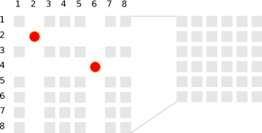
Analytical computation of the Bayesian recursive filtering presented above relies on the fact that permutations are observed completely. In tracking problems that would mean the algorithm has to receive observations (up to noise) of identities of every tracked object. This is a rare setting and most commonly observations are available only partially.

When a partial observation of $o$ objects becomes available, the dimension of the unknown part of $\mathbf{Y}$ is reduced from $n^{2}$ to $(n-o)^{2}$. The mechanism of this is shown in Figure 2, where circles indicate two observed objects and squares indicate the unknown parts of $\mathbf{P}$. The unknown part of the representation of $\mathbf{P}$ on $\mathbbm{S}^{d}$ needs to be marginalized out to obtain the likelihood used in (6). Figure 2 shows that this marginalization is straightforward in $\mathbbm{R}^{n^{2}}$ space. Unfortunately, to implement (7), we need to marginalize on the surface of the sphere, $\mathbbm{S}^{d}\subset\mathbbm{R}^{(n-1)^{2}}$ – a much more difficult task.

Denoting the orthogonal part of the basis in $\mathbbm{R}^{n^{2}}$ that represents the $\mathbbm{R}^{(n-1)^{2}}$ subspace by an $n^{2}\times(n-1)^{2}$ matrix $\mathbf{Q}$, we project into this subspace by:

(10) $$vec\left(\mathbf{Y}\right) =\mathbf{Q}^{T}vec\left(\mathbf{P-\frac{1}{n}\mathbbm{1}}\right).$$

In the case of a partial observation, we know which elements of the vector being projected are consistent with the observation and are not going to change and which elements can have any possible value. This allows us to split the resulting vector $\mathbf{Y}$ into

(11) $$\mathbf{Y}=\mathbf{Y}_{*}+\mathbf{Y}_{?},$$

where $\mathbf{Y}*$ and $\mathbf{Y}_{?}$ respectively denote the observed and unobserved parts.

The likelihood with the unknown observations marginalized out becomes:

(12) $$\frac{1}{Z}\int_{\mathbf{Y}_{?}}e^{\kappa_{1}\mathbf{Y}_{*}^{T}\mbox{\boldmath$x$}+\kappa_{1}\mathbf{Y}_{?}^{T}\mbox{\boldmath$x$}}d\mathbf{Y}_{?} =\frac{1}{Z}e^{\kappa_{1}\mathbf{Y}_{*}^{T}\mbox{\boldmath$x$}}\int_{\mathbf{Y}_{?}}e^{\kappa_{1}\mathbf{Y}_{?}^{T}\mbox{\boldmath$x$}}d\mathbf{Y}_{?}$$

Some details make computing the integral in (12) not totally trivial: $\mbox{\boldmath$x$},\mathbf{Y}_{*}$, and $\mathbf{Y}_{?}$ are of different length; although $x$ is fixed, $\mathbf{Y}_{*}$ and $\mathbf{Y}_{?}$ are not allowed to take any possible angle in $\mathbbm{R}^{(n-1)^{2}}$. We omit the details of the derivation dealing with these difficulties and just state the parameters of the resulting vMF likelihood function:

(13) $$\begin{split}\mbox{\boldmath$\mu$}&=\frac{\mathbf{Y}_{*}}{\|\mathbf{Y}_{*}\|_{2}}\end{split}\begin{split}\kappa&=\|\kappa_{1}\mathbf{Y}_{*}\|_{2}\end{split}$$

Thus, in the case of vMF we can execute a recursive Bayesian filter using only analytical computation even in the cases when only partially observed data is available. This makes the state space model applicable in a much wider range of scenarios than our initial model presented in Section LABEL:sec:cfo.

4. Experiments

(a)

(b)

Figure 3. Average error of a random hidden permutation inference from 100 (partial) noisy observations on 25 and 50 objects simulated datasets. Runs were repeated 10 times with a different permutation.

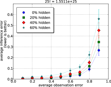
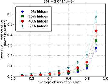
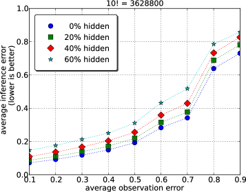
To demonstrate correctness of our approach, we show inference of a fixed hidden permutation from its noisy partial observations. Figure 3 shows results of this inference on dataset of 25 and 50 objects. In these first, synthetic data, experiments, we first randomly chose a true (hidden) permutation, $\mathbf{P}_{true}$. We controlled both observation noise ($\nu\in{0.1,0.2,...,0.9}$) and fraction of objects missing from observations ($m\in{0\%,20\%,40\%,60\%}$). Noisy observations were drawn from vMF($\mathbf{P}_{true}$,$\kappa_{\nu}$), where $\kappa_{\nu}$ was chosen to achieve $\nu$ fraction of incorrectly observed object identities. The final observation, $\mathbf{P}_{m}$, was generated by hiding $m$ percent of entries from the noisy observation matrix, chosen uniformly at random without replacement. Figure 3 shows that our representation of the $n!$ discrete permutation space is functional and the approach can gracefully handle large number of objects, partial observations and observation noise.

(a)

(b)

Figure 4. Tracking error on the air traffic control dataset for 6 and 10 planes as a function of observation noise shown as the fraction of incorrectly reported planes. Separate plots show error for partial observations when a fraction of object identities is unobserved.

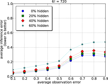
The above simulation was generated with the noise model used by the inference and did not have a temporal component, although it was applied to a really large state space. Next we show experiments on a tracking dataset with a non-vMF transition model. We use a dataset of planar locations of aircraft within a 30 mile diameter of John F. Kennedy airport of New York. The data, in streaming format, is available at http://www4.passur.com/jfk.html. The complexity of the plane routes and frequent crossings of tracks in the planar projection make this an interesting dataset for identity tracking. Identity tracking results on this dataset, in the context of the symmetric semigroup approach to permutation inference, were previously reported in [5]. Replicating the task reported in [5], we show results on tracking datasets of 6 and 10 flights, dropping the 15 flights dataset (but see below).

The dataset comes prelabeled, but the uncertainty is introduced by randomly swapping identities of flights $i$ and $j$ at their respective locations $\mbox{\boldmath$x$}_{i}$ and $\mbox{\boldmath$x$}_{j}$ with probability $p_{swap}exp(-\|\mbox{\boldmath$x$}_{j}(t)-\mbox{\boldmath$x$}_{i}(t)\|^{2}/(2s^{2}))$, where $p_{swap}=0.1$ and $s=0.1$ are strength and scale parameters respectively.

We then generated observation and hidden identity noise in the same way as for the prior experiment. Figure 4 shows results of applying our identity tracking method to the air traffic control dataset for various levels of observation noise and amount of missing identity observations. It is difficult to compare the performance to the method of [5] applied to the same dataset, since it is not clear how observation noise levels correspond to each other. However, error values reported in [5] were 0.12 to 0.17 on the 6 flights dataset and 0.2 to 0.32 on the 10 flights dataset. This is comparable to what we get with our approach for observation error below 50%, even when 60% of the flight identities are unobserved. Results of the application of our state space model to this dataset indicate robustness of the model to the choice of the transition model, which was different from the generative model of our tracking inference engine.

(a)

(b)

Figure 5. Tracking error on a football visual surveillance dataset for 41 players as a function of observation noise. Different missing data fractions are shown.

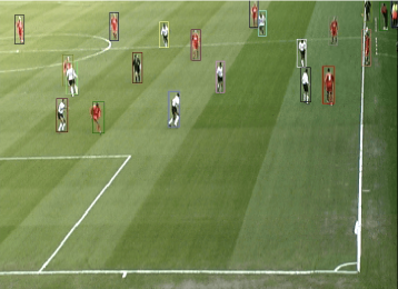
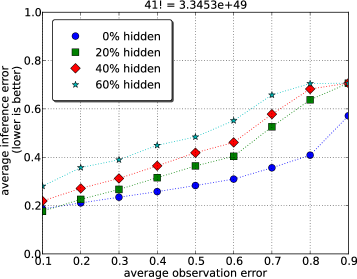
Due to the unmanageable size of the factorial space in identity tracking problems, even the powerful and efficient methods based on Fourier representation of permutations do not report results on more than 11 [4] or 15 [5] simultaneously tracked objects. The results of Figure 3 show that our approach can handle large numbers of objects, and Figure 4 demonstrated comparable accuracy on the air traffic control dataset. Next we show results on 41 objects from a visual surveillance dataset available from http://vspets.visualsurveillance.org/. Figure 5 shows an example of the underlying data and results of the identity tracking. The problem is similar to the above air traffic control: we have added uncertainty to the players, identities using the same exponential proximity model as before. Further, unlike the air traffic domain, here there are very few time steps that do not involve an identity swap. This kind of situation is difficult for recursive Bayesian filtering in general. However, our approach handles the situation and produces reasonable results with acceptable error rate – indeed, quite a good error rate, considering the size of the state space.

5. Conclusions

The main result of this work is embedding permutations into a continuous manifold, thus lifting a body of results from directional statistics field [8] to the fields of ranking, identity tracking and others, where permutations play essential role. Among many potential applications of this embedding we have chosen probabilistic identity tracking and were able to set up a state-space model with efficient recursive Bayesian filter that produced results comparable with the state of the art techniques very efficiently even on a very large datasets that pose difficulties to existing methods. There remains much to be done in this direction. However, a simple model, that can be thought of as a continuous generalization of the Mallows model [9, 2], equipped with results from the field of directional statistics has efficiently produced results of a reasonable accuracy. This is promising and encourages further development of more complicated probability distributions for permutations: further exploration of the exponential family already developed in the field [8] as well as developing more complex representations using spherical harmonics representations.

References

- [1] A. Chiuso and G. Picci. Visual tracking of points as estimation on the unit sphere. The confluence of vision and control, pages 90–105, 1998.
- [2] M. A. Fligner and J. S. Verducci. Distance based ranking models. Journal of the Royal Statistical Society. Series B (Methodological), 48(3):359–369, 1986.
- [3] R. E. Gomory. Outline of an algorithm for integer solutions to linear programs. Bulletin of the American Mathematical Society, 64(5):275–278, 1958.
- [4] J. Huang, C. Guestrin, and L. Guibas. Fourier theoretic probabilistic inference over permutations. Journal of Machine Learning (JMLR), 10:997–1070, May 2009.
- [5] R. Kondor, A. Howard, and T. Jebara. Multi-object tracking with representations of the symmetric group. In Proceedings of the Eleventh International Conference on Artificial Intelligence and Statistics, March 2007.
- [6] E. Kreyszig. Introductory Functional Analysis with Applications. John Wiley & Sons, 1978.
- [7] W. J. Lentz. Generating bessel functions in mie scattering calculations using continued fractions. Appl. Opt, 15:668–671, 1976.
- [8] K. V. Mardia and P. E. Jupp. Directional Statistics. John Wiley and Sons Ltd., 2 edition, 2000.
- [9] M. Meila, K. Phadnis, A. Patterson, and J. Bilmes. Consensus ranking under the exponential model. In Proceedings of the 23rd Annual Conference on Uncertainty in Artificial Intelligence (UAI), pages 285–294, Corvallis, Oregon, 2007. AUAI Press.
- [10] J. R. Munkres. Topology: A First Course. Prentice Hall, 1975.
- [11] T. E. S. Raghavan R. B. Bapat. Nonnegative Matrices and Applications. Encyclopedia of mathematics and its applications. cambridge University Press, 1997.
- [12] C. Rasmussen and G. D. Hager. Probabilistic data association methods for tracking complex visual objects. IEEE Transactions on Pattern Analysis and Machine Intelligence, 23(6):560–576, 2001.
- [13] D. B. West. Introduction to graph theory. Prentice Hall Upper Saddle River, NJ, 2001.