Prediction

Abstract

This chapter first presents a rather personal view of some different aspects of predictability, going in crescendo from simple linear systems to high-dimensional nonlinear systems with stochastic forcing, which exhibit emergent properties such as phase transitions and regime shifts. Then, a detailed correspondence between the phenomenology of earthquakes, financial crashes and epileptic seizures is offered. The presented statistical evidence provides the substance of a general phase diagram for understanding the many facets of the spatio-temporal organization of these systems. A key insight is to organize the evidence and mechanisms in terms of two summarizing measures: (i) amplitude of disorder or heterogeneity in the system and (ii) level of coupling or interaction strength among the system’s components. On the basis of the recently identified remarkable correspondence between earthquakes and seizures, we present detailed information on a class of stochastic point processes that has been found to be particularly powerful in describing earthquake phenomenology and which, we think, has a promising future in epileptology. The so-called self-exciting Hawkes point processes capture parsimoniously the idea that events can trigger other events, and their cascades of interactions and mutual influence are essential to understand the behavior of these systems.

chapter in “Epilepsy: The Intersection of Neurosciences, Mathematics, and Engineering” ,Taylor & Francis Group, Ivan Osorio, Mark G. Frei, Hitten Zaveri, Susan Arthurs, eds (2010)

1 A brief classification of predictability

Characterizations of the predictability (or unpredictability) of a system provide useful theoretical and practical measure of its complexity [9, 72]. It is also a grail in epileptology, as advanced warnings by a few minutes may drastically improve the quality of life of these patients.

1.1 Predictability of linear stochastic systems

Consider a simple dynamical system with the following linear auto-regressive dynamics

$$r(t)=\beta r(t-1)+\epsilon(t)~{},$$ (1)

where $0<\beta<1$ is a constant and $\epsilon(t)$ is a i.i.d. (independently identically distributed) random variable, i.e., a noise, with variance $\sigma_{\epsilon}^{2}$. The dependence structure between successive values of $r(t)$ is entirely captured by the correlation function which is non-zero only for the time lag of one unit step (in addition to the zero-time lag of course). Indeed, the correlation coefficient between the random variable at some time and its realization at the following time step is nothing but $\beta$. Correspondingly, the covariance of $r(t-1)$ and $r(t)$ is $\beta\times\sigma_{r}^{2}$, where $\sigma_{r}^{2}=\sigma_{\epsilon}^{2}/(1-\beta^{2})$ is the variance of $r(t)$. More generally, consider an extension of expression (1) into a linear auto-regressive process of larger order, so that we can consider an arbitrary covariance matrix $C(t,t^{\prime})$ between $r(t)$ and $r(t^{\prime})$ for all possible instant pairs $t$ and $t^{\prime}$. A simple mathematical calculation shows that the best linear predictor $m_{t}$ for $r(t)$ at time $t$, knowing the past history $r_{t-1},r_{t-2},...,r_{i},...$ is given by

$$m_{t}\equiv{1\over B(t,t)}\sum_{i<t}B(i,t)r_{i}~{},$$ (2)

where $B(i,t)$ is the coefficient $(i,t)$ of the inverse matrix of the covariance matrix $C(t,t^{\prime})$. This formula (2) expresses that each past values $r_{i}$ impacts on the future $r_{t}$ in proportion to its value with a coefficient $B(i,t)/B(t,t)$ which is non-zero only if there is non-zero correlation between the realization of the variable at time $i$ and time $t$. This formula (2) provides the best linear predictor in the sense that it minimizes the errors in a variance sense. Armed with this prediction, useful operational strategies can be developed, depending on the context. For instance, if the set $\{r(t)\}$ denotes the returns of a financial asset, then, one could use this prediction (2) to invest as follows: buy if $m_{t}>0$ (expected future price increase) and sell if $m_{t}<0$ (expected future price decrease).

Such predictor can be applied to general moving average and auto-regressive processes with long memory, whose general expression reads [41]

$$\left(1-\sum_{i=1}^{p}\phi_{i}L^{i}\right)\left(1-L\right)^{d}r(t)=\left(1+\sum_{j=1}^{q}\theta_{j}L^{j}\right)\epsilon(t)~{},$$ (3)

where $L$ is the lag operator defined by $Lr(t)=r(t-1)$ and $p,q$ and $d$ can be arbitrary integers. Such predictors are optimal or close to optimal as long as there is no change of regime, that is, if the process is stationary and the coefficients $\{\phi_{i}\}$ and $\{\theta_{j}\}$ and the orders of moving average $q$, of auto-regression $p$ and of fractional derivation $d$ do not change during the course of the dynamics. Otherwise, other methods, including Monte Carlo Markov Chains, are needed [41]. In the case where the initial conditions or observations during the course of the dynamics are obtained with noise or uncertainty, Kalman filtering and more generally data assimilation methods [58] provide significant improvements in predicting the dynamics of the system.

1.2 Predictability of low-dimensional deterministic chaotic systems

There is an enormous amount of literature on this subject since the last 1970s (see for instance [6, 74, 72, 89, 125] and references therein). The idea of how to develop predictors for low-dimensional deterministic chaotic systems is very natural: because of determinism, and provided that the dynamics is in some sense sufficiently regular, the short-time evolution remembers the initial conditions, so that two trajectories that are found in a neighborhood of each other remain close to each other for a time $t_{f}$ roughly given by the inverse of the largest Lyapunov exponent. Thus, if one monitors past evolution, however complicated, a future path which comes in the vicinity of a previously visited point will then evolve along a trajectory shadowing the previous one over a time of the order of $t_{f}$ [31, 127, 103]. The previously recorded dynamical evolution of a domain over some short-time horizon can thus provide in principle a short-term prediction through the knowledge of the transformation of this domain.

However, in practice, there are many caveats to this idealized situation. Model errors and noise, additive and/or multiplicative (also called “parametric”), complicate and limit predictability. Model errors refer to the generic problem that the used model is at best only an approximation of the true dynamics, and more generally neglects some possibly important ingredients, making prediction questionable.

In the simplest case of additive noise decorating deterministic chaotic dynamics, it turns out that the standard statistic methods for the estimation of the parameters of the model break down. For instance, the application of the maximum likelihood method to unstable nonlinear systems distorted by noise has no mathematical ground so far [98]. There are inherent difficulties in the statistical analysis of deterministically chaotic time series due to the tradeoff between the need of using a large number of data points in the maximum likelihood analysis to decrease the bias and to guarantee consistency of the estimation, on the one hand, and the unstable nature of dynamical trajectories with exponentially fast loss of memory of the initial condition, on the other hand. The method of statistical moments for the estimation of the parameter seems to be the unique method whose consistency for deterministically chaotic time series is proved so far theoretically (and not just numerically) [98]. But the method of moments is well-known to be relatively inefficient.

1.3 Predictability of systems with multiplicative noise

The presence of multiplicative (or parametric) noise makes the dynamics much richer… and complex. New phenomena appear, such as stochastic resonance [33], coherence resonance [97], noise-induced phase transitions [57, 116], noise-induced transport [42] and its game theoretical version, the Parrondo’s Paradox [1]. The predictability is then a non-monotonous function of the noise level. Even the simplest possible combination of nonlinearity and noise can utterly transforms the nature of predictability. Consider for instance the bilinear stochastic dynamical system, arguably the simplest incarnation of nonlinearity (via bilinear dependence on the noise) and stochasticity:

$$r(t)=\epsilon(t)+b\epsilon(t-1)\epsilon(t-2)~{},$$ (4)

where $\epsilon(t)$ is a i.i.d. noise. The dynamics (4) is the simplest implementation of the general Volterra discrete series of the type

$$r(t)=H_{1}\left[\epsilon(t)\right]+H_{2}\left[\epsilon(t)\right]+H_{3}\left[\epsilon(t)\right]+...+H_{n}\left[\epsilon(t)\right]+...$$ (5)

where

$$H_{n}\left[\epsilon(t)\right]=\sum{j_{1}=0}^{+\infty}...\sum{j_{n}=0}^{+\infty}h_{n}(j_{1},...,j_{n})\epsilon(t-j_{1})...\epsilon(t-j_{n})~{}.$$ (6)

By construction, the time series $\{r(t)\}$ generated by expression (4) has no linear predictability (zero two-point correlation) but a certain nonlinear predictability (non-zero three-point correlation) [99]. It can thus be considered as a paradigm for testing the existence of a possible nonlinear predictability in a given time series. Notwithstanding its remarkable simplicity, the bilinear stochastic process (4) exhibits remarkably rich and complex behavior. In particular, the inversion of the key nonlinear parameter $b$ and of the two initial conditions necessary for the implementation of a prediction scheme exhibits a quite anomalous instability: in the presence of a some random large impulse of the exogenous noise $\epsilon(t)$, the ensuing dynamics exhibits super-exponential sensitivity for the inversion of the innovations [99].

1.4 Higher dimensions, coherent flows and predictability

Going bottom-up in the complexity hierarchy, we have low-dimensional chaos $\to$ spatio-temporal chaos [19] $\to$ turbulence [30]. It turns out that, contrary to naive expectation, increasing dimensionality and introducing spatial interactions does not necessary destroy predictability. This is due to the organization of the spatio-temporal dynamics in so-called “coherent structures”, corresponding to coherent vortices in hydrodynamic flows [8]. It has been shown that the full nonlinearity acting on a large number of degrees of freedom can, paradoxically, improve the predictability of the large scale motion, giving a picture opposite to the one largely popularized by Lorenz for low-dimensional chaos. The mechanism for improved predictability is that small local perturbations can progressively grow to larger and larger scales by nonlinear interaction and finally cause macroscopic organized persistent structures [100].

1.5 Fundamental limits of predictability and the virtue of coarse-graining

Algorithmic information theory [76] combines information theory, computer science and meta-mathematic logic. In the context of system predictability, it has profound implications. Indeed, a central result of algorithmic information theory obtained as a synthesis of the efforts of R. Solomonoff [126], A. Kolmogorov, G. Chaitin [11], P. Martin-Löf, M. Burgin and others states roughly that “most” dynamical systems evolve according to and/or produce outputs that are utterly unpredictable. Here, the term “most” in “most dynamical systems” mean that this property holds with probability $1$ when choosing at random a dynamical system from the space of all possible dynamical systems. Specifically, the data series produced by most dynamical systems have been proved to be computationally irreducible, i.e. the only way to decide about their evolution is to actually let them evolve in time. There is no way you can compress their dynamics and the resulting information into generation rules or algorithms that are shorter than the output itself. Then, the only strategy is to let the system evolve and reveal its complexity, without any hope of predicting or characterizing in advance its properties. The future time evolution of most complex systems thus appears inherently unpredictable. This is the foundation for the approach pioneered by S. Wolfram [162] to basically renounce the hope to get mathematical laws and predictability, and replace them by the search for cellular automata that have universal computational abilities (like so-called Turing machines) and can reproduce any desired pattern.

Such views are almost shocking to most scientists, whose job is to find patterns that can be captured in coherent models that provide a reduced encoding of the observed complexity, in direct apparent contradiction with the central result of algorithmic information theory. Israeli and Goldenfeld have provided an insightful and elegant procedure, based on renormalization group theory, to reconcile the two view points [60, 61]. The key idea is to ask only for approximate answers, which for instance makes physics work, unhampered by computational irreducibility. By adopting the appropriate “coarse-grained” perspective of how to study the system, Israeli and Goldenfeld found that even the known computational irreducible cellular automaton (rule 110 in Wolfram’s classification [161]) becomes relatively simple and predictable. In physics, this comes as no surprise. Each trajectory of the approximately $10^{25}$ molecules in an office room each follows an utterly chaotic trajectory, which loses predictability after a few inter-molecular collisions. But the coarse-grained large-scale properties of the gas is well-captured by the law of ideal gas $pV=nRT$, or van der Waals’ equation if one wants a bit more precision, where $p$ is the pressure in the enclosure of volume $V$ at temperature $T$, and $n$ is the number of moles of gas, while R is a constant. Thus, but asking questions involving different scales, computationally irreducible systems can be predictable at some level of description. The challenge is to find how to coarse-grain, what is the optimal level of description, and what effective macroscopic interactions and patterns emerge from this procedure. There are promising developments in this direction to elaborate a general theory of hierarchical dynamics [84, 39, 24], using the renormalization group as a constructive meta-theory of model building [160].

1.6 “Dragon-kings”

Predictability may come from another source, that is, directly from specific transient structures developing in the system, that we refer to as “dragon-kings” [137, 117].

The concept of dragon-kings has been introduced as a frontal refutal to the claim that “black swans” characterize the dynamics of most systems [155]. According to the “black swan” hypothesis, highly improbable events with extreme sizes or impacts are thought to occur randomly, without any precursory signatures. “Black swan” events are thought to be events of large sizes associated with the tail of distributions such as power laws. Because the same power law distribution is thought to describe the whole population of event sizes, including the “black swans” of great impact, the argument is that there are not distinguishing features for these “black swans”, except their great sizes, and therefore no way to diagnose their occurrence in advance. In this story, for instance, a great earthquake is just an event that started as a small earthquake… and did not stop growing. Its occurrence is argued to be inherently unpredictable because there is not way to distinguish the nucleation of the myriads of small events from the rare ones that will grow to great sizes by chance [35].

In contrast, the “dragon-king” hypothesis proposes that extreme events from many seemingly unrelated domains may be plausibly understood as part of a different population than that comprising the large majority of events. This difference may result from amplifying mechanisms, such as positive feedbacks, which are active only transiently, leading to the emergence of non-stationarity structures. The term “dragon” refers to the mythical animal that belongs to a different animal kingdom beyond the normal, with extraordinary characteristics. The term “king” had been introduced earlier [75] to emphasize the importance of those events, which are beyond the extrapolation of the fat tail distribution of the rest of the population. This is in analogy with the sometimes special position of the fortune of kings, which appear to exist beyond the Pareto law distribution of wealth of their subjects [137]. The concept of dragon-kings has been argued to be relevant under a broad range of conditions in a large variety of systems, including the distribution of city sizes in certain countries such as France and the United Kingdom, the distribution of acoustic emissions associated with material failure, the distribution of velocity increments in hydrodynamic turbulence, the distribution of financial drawdowns, the distribution of the energies of epileptic seizures in humans and in model animals, the distribution of the earthquake energies and the distribution of avalanches in slowly driven systems with frozen heterogeneities (see [137, 117] for a detailed presentation of these various examples and the related bibliography).

1.7 A Landau-Ginzburg model of self-organized critical avalanches coexisting with Dragon-kings

The following model [36] provides a quite generic set-up for the emergence of dragon-kings under wide parameter conditions, coexisting with a self-organized critical regime under different parameter conditions. This model is relevant to a large number of systems, including systems of coupled neurons. Consider an extended system, whose local state at position ${\vec{r}}$ and time $t$ is characterized by the local order parameters $S({\vec{r}},t)$. The order parameter $S$ is zero in absence of activity and non-zero otherwise. Its amplitude $S({\vec{r}},t)$ quantifies the level of activity at ${\vec{r}}$ and time $t$.

The simple and general dynamical equation that captures the process of jumps between a zero to a non-zero activity state consists of the normal form of the sub-critical pitchfork bifurcation of co-dimension $1$:

$${\partial S\over\partial t}=\chi\left(\mu S+2\beta S^{3}-S^{5}\right)~{}.$$ (7)

The parameter $\chi$ sets the characteristic time scale $1/\chi$ of the dynamics of $S$. The parameter $\beta$ is taken positive, corresponding to the sub-critical pitchfork bifurcation regime. In absence of the stabilizing $-S^{5}$ term, the non-zero fixed points (for the relevant regime $\mu<0$) given by $S^{*}_{\pm}=\pm\sqrt{-\mu/2\beta}$ are unstable, while the fixed point $S_{0}=0$ is locally stable. These two unstable fixed points correspond to the dashed line in figure 1. The term “locally” reflects the fact that a sufficiently large perturbation that pushes $S$ above $S^{*}_{+}$ or below $S^{*}_{-}$ will be amplified leading to a diverging amplitude $|S|$ at long times. In the presence of the $-S^{5}$ term, two new fixed point exist, which are stable. They correspond to the upper solid line in figure 1. The bifurcation diagram of these fixed points as a function of $\mu$ shown in figure 1 is similar to the bifurcation diagram of the Hodgkin-Huxley model, for which the transmembrane voltage is the order parameter $S$ and the external potassium concentration is the control parameter $\mu$.

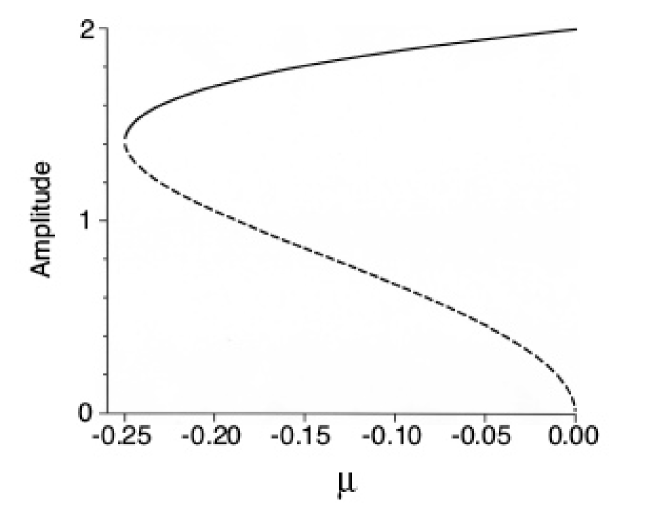
Figure 1: Bifurcation diagram in the positive domain $S>0$ of the normal form (7) plotting the amplitude $|S|$ as a function of the control parameter $\mu$.

Now, imagine that the normal form (7) describes the local state $S({\vec{r}},t)$ at ${\vec{r}}$ and time $t$, which may be different from point to point because the control parameter $\mu$ is actually dependent on position ${\vec{r}}$ and time $t$. We thus have as many dynamical equations of the form (7) as there are points ${\vec{r}}$ in the system. For each point ${\vec{r}}$, the local control parameter $\mu({\vec{r}},t)$ is assumed to be an affine function of the gradient of a local concentration $h$:

$$\mu(r,t)=g_{c}-{\partial h\over\partial r}~{}.$$ (8)

We consider a cylindrical (or one-dimensional) geometry so that a single spatial coordinate $r$ is sufficient (and we can drop the arrow on ${\vec{r}}$). Here, $g_{c}$ is the critical value of the gradient at which the zero-fixed point $S_{0}=0$ becomes linearly unstable. The model in Ref. [36] assumed a slightly different technical form ($\mu(r,t)=g_{c}-\left({\partial h\over\partial r}\right)^{2}$), which does not change the main regimes and results described below.

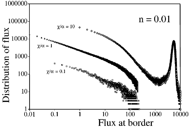
Figure 2: Distribution of flux amplitudes at the open border of the one-dimensional system obeying the dynamics described by expressions (7,8,9,10). The standard deviation $n$ of the noise term $n(r,t)$ is equal to $0.01$ (small driving noise regime). Reproduced from Ref. [36].

Because we think of $h(r,t)$ as a diffusing field, its equation of evolution is generically

$${\partial h\over\partial t}=-{\partial F\left(S,{\partial h\over r}\right)\over\partial r}+n(r,t)~{}.$$ (9)

This equation expresses that the rate of change of $h$ is equal to the gradient of a flux that ensures the conservation of the concentration, up to an external fluctuation noise $n(r,t)$ acting on the system. The last ingredient of the model consists in writing that the flux is proportional to the gradient of the field:

$$F\left(S,{\partial h\over r}\right)=-\alpha~{}S^{2}~{}{\partial h\over\partial r}~{},$$ (10)

where $\alpha$ is another inverse time scale controlling the diffusion rate of the field within the system. The proportionality between the flux $F$ and the gradient $-{\partial h\over\partial r}$ of the field is simply Fick’s law. The non-standard ingredient stems from the fact that the coefficient of proportionality, usual defining the diffusion coefficient, is controlled by the amplitude $S^{2}$ of the order parameter. In absence of activity $S=0$, the local flux $F$ is here zero and the field does not change, up to noise perturbations. This corresponds to a strong feedback of the order parameter onto the control parameter, which has been shown to be one of the possible mechanism for the emergence of self-organized criticality [130, 29, 36]. Recall that standard formulations of the dynamics and bifurcation patterns of evolving systems in terms of normal forms assume the existence of control parameters that are exogenously determined. Here, the order parameter of the dynamics has an essential role in determining the value of the control parameter, which becomes itself an endogenous variable.

The analysis of the dynamics described by expressions (7,8,9,10) presented in Ref. [36] shows that a self-organized critical (SOC) regime [5] appears under the condition of small driving noise and when the diffusive relaxation is faster than the instability growth rate: $\alpha>\chi$. The SOC dynamics can be shown to be associated with a renormalized diffusion equation at large scale with an effective negative diffusion coefficient [36], expressing that small scale fluctuations are the most unstable and cascade intermittently to large scale avalanches. This SOC regime is exemplified by the power law distributions of avalanche sizes shown in figure 2 for $\chi/\alpha=0.1$ and $1$. More interesting for our purpose is the fact that, when $\alpha<\chi$, characteristic large scale events appear, which coexist with a crowd of smaller events themselves approximately distributed according to a power law with an exponent larger than in the SOC regime. The dragon-kings correspond to the peak on the right of figure 2, associated with the run-away avalanches of size comparable to the size of the system.

This constitutes an example of what we believe to be a generic behavior found in systems made of heterogeneous coupled threshold oscillators, such as sandpile models, Burridge-Knopoff block-spring models [120] and earthquake-fault models [144, 145, 20]: a power law regime (self-organized critical) (Figure 11, right lower half) is co-extensive with one of synchronization [153] with characteristic size events (Figure 11, upper left half). We discuss below this generic phase diagram, in our attempt to compare the dynamics and resulting statistical regularities observed in earthquakes, financial fluctuations and epileptic seizures.

1.8 Bifurcations, Dragon-kings and predictability

The existence of “dragon-kings” punctuating the dynamics of a given system suggests mechanisms of self-organization otherwise not apparent in the distribution of their smaller siblings. Therefore, this opens the potential for predictability, based on the hypothesis that these specific mechanisms that are at the origin of the dragon-kings could leave precursory fingerprints usable for forecasts.

The dynamical system (7,8,9,10) presented in the previous section shows an example in which the dragon-kings appear in a large range of parameters in the presence small scale subcritical bifurcation dynamics, which are renormalized at large scales into a change of regime, a bifurcation of behavior, more generally a transition of phase. In other words, dragon-kings are commonly associated with a phase transition. If a phase transition can be detected before it occurs, it may be understood as an abrupt increase in the probability, or risk, of an extreme event. Practical examples include ruptures in materials and bursting of financial bubbles.

Mathematicians have proved [156, 4] that, under fairly general conditions, the local study of bifurcations of almost arbitrarily complex dynamical systems can be reduced to a few archetypes. More precisely, it is proved that there exists reduction processes, series expansions and changes of variables of the many complex microscopic equations such that, near the fixed point (i.e. for small values of the order parameter $S$), the behavior is described by a small number of ordinary differential equations depending only a few control parameters, like $\mu$ in expression (7) for a sub-critical pitchfork bifurcation. The result is non-trivial since a few effective numbers such as $\mu$ represent the values of the various relevant control variables and a single (or just a few) order parameter(s) is(are) sufficient to analyze the bifurcation instability. The remarkable consequence is that the dynamics of the system in the vicinity of the bifurcation is reducible and thus predictable to some degree. This situation can be described as a reduction of dimensionality or of complexity, that occurs in the vicinity of the bifurcation. Such reduction of complexity may occur dynamically and intermittently in large dimensional out-of-equilibrium systems, such as in hierarchically coupled Lorenz systems [78] or in agent-based models of financial markets [2].

As an illustration, consider expression (7) where $\beta$ is now assumed negative. Since the cubic term $2\beta S^{3}$ is now stabilizing, the quintic term $-S^{5}$ can be dropped. An interesting so-called super-critical bifurcation occurs at $\mu=0$, separating the regime for $\mu<0$ where the zero-fixed point $S_{0}=0$ is unique and is stable, from the regime $\mu>0$ where two symmetric stable fixed points appear at $S^{*}_{\pm}=\pm\sqrt{\mu/2|\beta|}$, and the zero-fixed point $S_{0}=0$ becomes unstable. Consider the dynamics of such a system slightly perturbed by an external noise $n(t)$ with zero mean and variable $\sigma^{2}$, so that its dynamics reads

$${dS\over dt}=\mu S-2|\beta|S^{3}+n(t)~{}.$$ (11)

For $\mu<0$, the average value $\langle S(t)\rangle$ vanishes but its variance can be calculated explicitly from the solution of (11). Indeed, to a very approximation, we can drop also the $2|\beta|S^{3}$ term since $S$ is exhibiting only small fluctuating excursions around $0$, for $\mu<0$, according to

$$S(t)=\int_{-\infty}^{t}e^{-|\mu|(t-\tau)}~{}n(\tau)d\tau~{}.$$ (12)

Its variance $\langle[S(t)]^{2}\rangle$ is then given by

$$\langle[S(t)]^{2}\rangle=\sigma^{2}\int_{-\infty}^{t}e^{-2|\mu|(t-\tau)}d\tau={\sigma^{2}\over 2|\mu|}~{}.$$ (13)

This result (13) shows that the variance $\langle[S(t)]^{2}\rangle$ of the fluctuations of the order parameter diverges as the critical bifurcation point is approached from below: $\mu\to 0^{-}$. $\langle[S(t)]^{2}\rangle$ plays the role of a susceptibility, whose divergence on the approach to the critical point suggests a general predictability, for instance obtained by monitoring the growth and correlation properties of the system fluctuations. This method has been used in particular for material failure (recording of micro-damage for instance via acoustic emissions) [3, 34, 64], human parturition (proposed recording of the mother-foetus maturation process via Braxton-hicks contractions of the uterus) [139, 138], financial crashes (monitoring of bursts of price acceleration and various risk measures via options) [141, 63, 65, 134] and earthquakes (monitoring of precursory seismic, electromagnitic and chemical activity) [147, 66, 10]. We believe that this phase transition approach bears great potential to predict catastrophic events, recognizing precursors in time series associated with finite-time singularities [62, 115, 59, 37], hierarchical power law precursors [133], critical slowing down [21] and other types of precursors [136, 119].

2 Parallels between earthquakes, financial crashes and epileptic seizures

How can the concepts described in the previous section be applied to real systems, and in particular to the prediction of epileptic seizures? To put this question in a broader perspective, we present in this section an original attempt [91, 92] to draw parallels between seemingly drastically different systems and phenomena, based on both qualitative and quantitative evidence.

2.1 Introduction to earthquakes, financial crashes and epileptic seizures

Earthquakes occur mostly in the thin upper fragile layer of the Earth, called the upper crust. A complex system of slowly moving tectonic plate boundaries delineate their most probable location, as shown in figure 3. Recent syntheses of compendium of geological and seismic data [7] suggest that the system of tectonic plates covering the Earth surface is “fractal” [146], i.e., composed of a broad (power law) distribution of plates. Even more interesting is the fact that, in broad region around the tectonic plate boundaries, earthquakes are clustered on networks of faults forming rich hierarchical structures from the thousand kilometer scale to the meter scale and below [94], as shown in figure 4. At a qualitative level (and supported quantitatively by some models [144, 79]), it is thought that the fault networks are self-organized by the repetitive action of earthquakes.

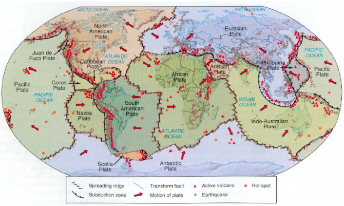
Figure 3: Standard model of 12 major tectonic plates showing their relative motions (thick red arrows), and the plate boundaries which concentrate a large fraction of seismic and volcanic activity. The three types of the place boundaries are also indicated in the legend.

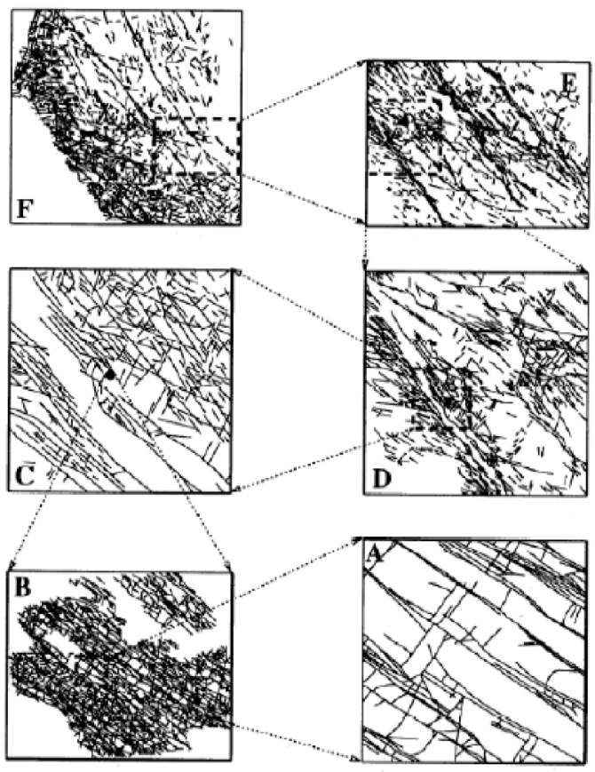
Figure 4: Example illustrating the hierarchical organization of faults from the 400 km scale (upper left panel) down to the 1 meter scale (lower right panel). Reproduced from ref. [94].

Financial crashes occur in organized markets trading assets, such as equities of firms, commodities such as oil or gold, and bonds (debts of firms or of countries). By their varying and heterogeneous demand and supply, investors are responsible for the observed price variations. Investors come in a very broad distribution of sizes (and therefore market impacts), from the individual private household to the largest pension and mutual funds, commanding up to hundreds of billions of dollars. These investors are interacting with other investors as well as with market makers, with commercial and investment banks, as well as more recently with sovereign funds. This variety of sizes, needs and goals provides a fertile ground for rich behaviors, including systemic instabilities and crippling crashes.

Epileptic seizures occur within what many refer exaggeratedly to as the most complex system of this universe, the human brain. The human brain is organized in an exceedingly rich set of topographic and functional divisions at many scales, from the lobes and complex folded structures down to columns and to neurons (see figure 5 for a partial insight in this rich organization). The networking and function of these units reflect both encoded development programs as well as the impact of learning and experience that feedback on the development processes.

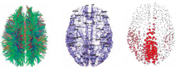
Figure 5: Illustration of the complex hierarchical network structure of the brain. Left: fiber pathways of the human cerebral cortex; middle: network of connections in the human cortex, with lines between brain regions indicating the strengths of the connections; right: location of highly connected hub nodes forming the structural core. Reproduced from Ref. [40].

2.2 Common properties between earthquakes, financial crashes and epileptic seizures

Earthquakes, financial crashes and epileptic seizures are characterized by several strikingly similar mechanisms and properties.

1. They occur on hierarchically organized structures, with many inter-connected scales.

2. Their distribution in sizes are heavy tailed and extreme events are typical.

3. There is a strong entanglement between the growth and properties of the supporting structures and the spatio-temporal organization of the events themselves: the supporting structures and the events inter-organize as in a chicken-and-egg problem: earthquakes occur on faults and faults grow and form networks shaped by the repetition of earthquakes; financial crashes occur on financial markets acted by investors whose actions and impacts result from the cumulative growth of their fortunes shaped by past financial performance, which feedbacks on future performance. Young brains grow with epileptic regimes (e.g., “absence” seizures) and there are many feedbacks between structures and functions. This suggests that a genuine understanding of the generating processes and of the properties of earthquakes, financial crashes and epileptic seizures can only be obtained by studying the joint organization of these events and their evolving self-organized carrying structures. The basis (bases) for this important statement is (are) not well developed for seizures.

4. Past earthquakes trigger future earthquakes: it is estimated that between 50% to close to 100% of earthquakes are triggered by past earthquakes (and not just the aftershocks). This is illustrated by the concept that earthquakes have “conversations”, similarly to the exchanges between different areas of the brain when developing cognitive tasks (see figure 6). Most of the volatility of financial markets is probably the result of endogenous amplification of past returns on future returns rather than the direct exogenous effect of external news, as for instance exemplified by the so-called “excess volatility” effect. The concept that seizures beget seizures has a long history and new recent empirical evidence supports the rational to revisit this hypothesis [91, 92].

5. Within a coarse-grained approach to the modeling of these systems, they can be represented as made of coupled threshold oscillators of relaxation (faults going to rupture, investors going to investment decisions, neurons going to a firing state).

6. There is some evidence that these three systems are characterized by the coexistence of scaling (power law distribution of event sizes) and regimes with large characteristic events [137].

7. Finally, there is a lot of interest in our modern societies to diagnose and predict large catastrophic events, to help alleviate the damage associated with earthquakes, the losses of financial crashes and to help patients recover normal lives in the presence of intermittent seizures.

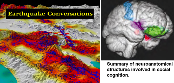
Figure 6: Left panel: cover picture of the Scientific American journal in with R.S. Stein [152] reviews the evidence for “earthquake conversations”, that is, the predominant hypothesis that earthquakes trigger earthquakes. The right panel outlines several important structures involved in social cognition and interactions (ventromedial prefrontal cortex (green), amygdala (red), right somatosensory cortex (blue) and insula (purple)). Reproduced from Ref. [40].

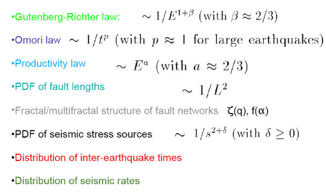
Figure 7: Survey of the major statistical laws in seismicity. The color code allows for comparison with the statistical laws in finance markets and in epileptic seizures documented in figures 8 and 9.

Figure 7 summarizes the main statistical laws that have been documented in seismology (see Ref. [129] and references therein).

1. The Gutenberg-Richter law describes the probability density function (pdf) of earthquakes of a given energy $E$, as being a power law with a small exponent $\beta\approx 2/3$.

2. The Omori law states that the rate of aftershocks following an earthquake (usually improperly referred to as a “main shock”) exhibits a burst immediately after the main shock and decays slowly in time afterwards as the inverse of time raised to an exponent $p$, which is close to $1$ for large earthquakes.

3. The productivity law describes how the average number of triggered earthquakes depend on the energy $E$ of the triggering earthquake: the larger an earthquake, the more earthquakes it triggers, according to a power law with an exponent $a$ probably slightly smaller than $\beta$ [46].

4. Because earthquakes occur on faults, and faults grow by earthquakes, it is important also to characterize the properties of fault networks. It is well-documented that the probability density distribution $P(L)$ of fault lengths in a given area is described by a power law $P(L)\simeq 1/L^{f}$ with exponent $f$ not far from $2$.

5. Several studies have documented that fault networks exhibit fractal, multifractal or better multi-scale hierarchical properties [94].

6. Earthquakes result from deformations that produce complex stress fields, which are one of the important fields at the origin of the nucleation of earthquakes (the distribution of water (brine) in the crust is also thought to play a crucial role, albeit we have only indirect and incomplete information, see Refs. [131, 132] for a review). The distribution of stress amplitudes have been documented from the focal source mechanism of earthquakes to be close to a Cauchy distribution, i.e., with a power law tail $\simeq 1/s^{2+\delta}$ and $\delta$ small [69].

7. The distribution of waiting times between earthquakes in a given region is also characterized by a fat tail, approximately quantified by a power law, indicative of a broad range of inter-event intervals. However, recent studies suggest that the pdf of inter-earthquake intervals has several regimes (see Ref. [111, 113, 149] and references therein) and may not be describable by a simple power law.

8. The distribution of seismic rates (number of earthquakes per unit time) in fixed regions is also well-described by a power law function [109].

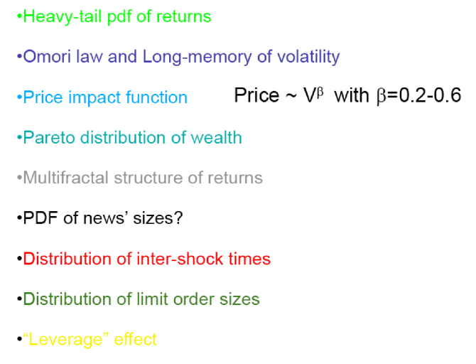
Figure 8: Survey of the major statistical laws in financial markets. The color code allows for comparison with the statistical laws in seismicity and in epileptic seizures documented in figures 7 and 9.

Figure 8 presents the most important statistical laws that characterize the regularities found in financial time series of returns.

1. The distribution of financial returns (or relative price variations) is fat-tailed, with a tail approximately described by a power law, but the exponent is in the range $2-4$ and thus much larger than for earthquake energies (whose exponent is $\simeq 2/3$). Hence, the returns have a well-defined and variance.

2. The relaxation of the level of activity of price fluctuations (called financial volatility) after a burst is also found to decay approximately as a power law [77, 143], similarly to the Omori law of earthquake aftershocks.

3. The analog of the productivity law of earthquake is the “price impact function” which relates the price change to the volume of stocks of a given transaction: the larger the demand for a stock, the more the price is pushed up.

4. Prices fluctuate because investors place orders. The size of the orders play in important role, as just said. The sizes of orders are obviously related to the “sizes” of the investors: a large mutual fund managing $100$ billion dollars has much more impact on the market that an individual managing a modest portfolio. The size distribution of individuals’ wealth, of firm sizes, of mutual fund portfolios, or university endowments are all found to be power laws. Characterizing the distributions by the probability density function (pdf), it is found of the form $\simeq 1/W^{f}$ with exponent close to $2$, which corresponds to Zipf’s law [107]. For such exponents, the mean is either not defined or converge poorly in typical statistical estimations.

5. The size distribution of portfolios plays a role similar to the fault distribution in earthquakes: portfolio sizes impact the size and nature of orders that move prices; reciprocally, the cumulative effect of price moves controls the performance of investment portfolios, and thus whether the size increases or decreases. We encounter again the chicken-and-egg structure.

6. There is also ample evidence that financial time series of returns are characterized by multifractal scaling.

7. The analogy of stress would be news but we are only starting to understand what is a “news” size and how to quantify it via the response function of social networks (see [104, 23, 135, 18]).

8. The distribution of time intervals between high levels of volatility has a similar structure as the inter-earthquake time distribution.

9. The distribution of limit-order sizes, analogous to the distribution of seismicity rates, is also a power law [38, 32].

10. However, the so-called “leverage effect”, in which past losses (large negative returns), tend to increase future volatility (and not reciprocally) [96], does not seem to have any counterpart in seismicity.

Figure 9: Survey of the major statistical laws known in epileptology. The color code allows for comparison with the statistical laws in seismicity and in financial markets documented in figures 7 and 8.

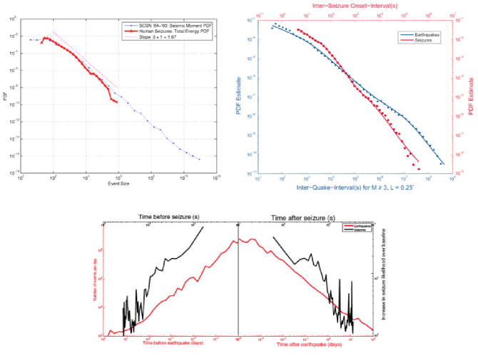
Figure 10: Upper left panel: Empirical probability density function (pdf) estimates of seismic moments (SCSN catalog; 1984-2000) (blue curve) and of seizure energies of 60 human subjects (red curve) originating from different epileptogenic regions. Upper right panel: empirical probability density function estimates of the inter-event times between earthquakes (blue circles; blue lower left scales) and seizures in humans (red circles; red upper right scales). Lower panel: superimposed epoch analysis of seizures (red line) and earthquakes (blue line) to test for the existence in seizures of “aftershocks” (Omori-like behavior) and “foreshocks” (inverse Omori-like behavior). Reproduced from Ref. [92].

Figure 9 reviews a number of statistical laws that have been found to characterize “focal” seizures in humans and generalized seizures in animals [91, 92].

1. The analogy with earthquakes is particularly striking for the Gutenberg-Richter distribution of event sizes, the Omori and inverse Omori laws, and the distribution of inter-event intervals, as shown in figure 10.

2. While these events occur in drastically different systems, they may nevertheless be described at a coarse-grained level by similar models of coupled heterogeneous threshold oscillators of relaxation: this provides an inspiration to investigate the possible existence of other statistical laws, such as productivity. One can suspect that the triggering ability of a seizure to promote another future seizures [91, 92] might depend on its duration, amplitude and/or energy. This remains to be tested.

3. We have already mentioned the hierarchical structure of the brain, as the structure supporting the spatio-temporal organization of brain activities and the seizures. But it is not known whether it can be characterized with multifractal properties.

4. The analog to stress sources in earthquakes would be the electric current field within the brain or gaba or other chemical compound concentration fields. It remains to be quantified whether these fields present interesting statistical properties, that may be used to better constrain modeling and perhaps be used for diagnostic.

5. The distribution of seizure rates has neither yet been quantified in a systematic manner.

6. And there is no obvious analogy with the leverage effect in finance. It is possible that for similar asymmetric dynamical effects exist, which would reveal at a collective level the asymmetry between excitatory and inhibitory processes in the brain.

2.3 Rationals for the analogy between earthquakes, financial crashes and epileptic seizures

The previous section has documented (and also extended conjectures on) a number of quantitative and qualitative correspondences between earthquakes, financial crashes and seizures. It is perhaps a priori counter-intuitive to compare earthquakes, financial fluctuations and seizures (the events), or fault networks, financial markets and neuron assemblies (the events’ supporting structures), due to the systems’ large differences in scales and in their constituent matter. However, the proposed correspondence may be motivated and at least partially explained on the grounds that these phenomena occur in systems composed of interacting heterogeneous threshold oscillators.

Consider first the textbook model of an earthquake represents a single fault slowly loaded by cm/year tectonic deformations until a threshold is reached at which meter-scale displacements occur in seconds. This textbook model ignores the recent realization that earthquakes do not occur in isolation but are part of a complex multi-scale organization in which earthquakes occur continuously at all spatio-temporal scales according to a highly intermittent, frequent energy release process [70, 95]. Indeed, the Earth crust is in continuous jerky motion almost everywhere but due to the relative scarcity of recording devices, only the few sufficiently large ones are detected, appearing as isolated events. In this sense, the dynamics of earthquakes is similar to the persistent barrages of subthreshold oscillations and of action potentials in neurons, which sometimes coalesce into seizures.

Market investors continuously place limit and market orders, with buyers (respectively sellers) tending to push prices up (respectively down). Early on, Takayasu et al. [154] noticed that trading strategies lead to dynamics belonging to the larger class of threshold dynamics with mean-reversal behavior, akin to the outcome of coupled threshold oscillators of relaxation. Traders and investors enter and exit financial markets at many different time scales, from milliseconds for the most modern electronic automatic platforms to years for investors with long horizons. The evolution of their impact is on the order of years, which is the time scale for growth or decay of fortunes. Furthermore, market rules and regulations, such as the Glass-Steagall act of 1932-33 or the Sarbanes-Oxley act of 2002, appear as reactions to extreme market regimes such as financial crashes (the 1929 crash and ensuing depression for the former and the accounting scandals revealed by the collapse of market capitalization of new technology firms in 2000), illustrating another process for the evolution of supporting structures co-evolving to the dynamics of events.

The separation of time scales in epileptogenic neuronal assemblies is similar (milliseconds to years) to financial markets (milliseconds to years), but smaller than in fault networks (fraction of seconds to millenia), but the organization of coupled threshold oscillators is not very sensitive to the magnitude of the separation of time scales, as long as there is one, a property that characterizes relaxational processes.

The term “relaxational process” is here applied to phenomena with a disproportionately long (hours to years) charging/loading process vis-a-vis the very short (seconds to minutes) discharge of the accumulated seismic energy, money/assets or neuronal membrane potentials. For instance, in the case of earthquakes, the slow motion of tectonic plates at typical velocities of a few cm/year accumulates strains in the core of locked faults over hundreds to thousands of years, which are suddenly relaxed by the meter-size slips occurring in seconds to minutes that define large earthquakes. Thus, one fault taken in isolation is genuinely a single relaxation threshold oscillator, alternating long phases of loading and short slip relaxations (the earthquakes). While less well studied than earthquakes, the long (hours to years) interval between seizures and their short duration (rarely over 2 min) interpreted in light of the fact that the brain is composed of relaxational threshold oscillators (neurons) supports the notion that seizures too are also relaxational phenomena. The relaxation nature of investment dynamics can be seen as the result of the competition between different strategies available to each investor and their collective output. This is particularly evident for first-entry games [101] and minority games [12, 16], in which agents with bounded rationality are continuously oscillating between different strategies, creating collectively large market price fluctuations and crashes.

2.4 Generic phase diagram of coupled threshold oscillators of relaxation

It is well-known in statistical physics and in dynamical systems theory that ensembles of interacting heterogeneous threshold oscillators of relaxation generically exhibit self-organized behavior with non-Gaussian statistics [105, 164, 73]. The cumulative evidence presented in figures 7, 8 and 9 provides a strong case for the dynamical analogy between earthquakes, financial fluctuations and seizures, i.e., the existence of an underlying universal organization principle captured by the sand pile avalanche paradigm and the concept of self-organized criticality [5].

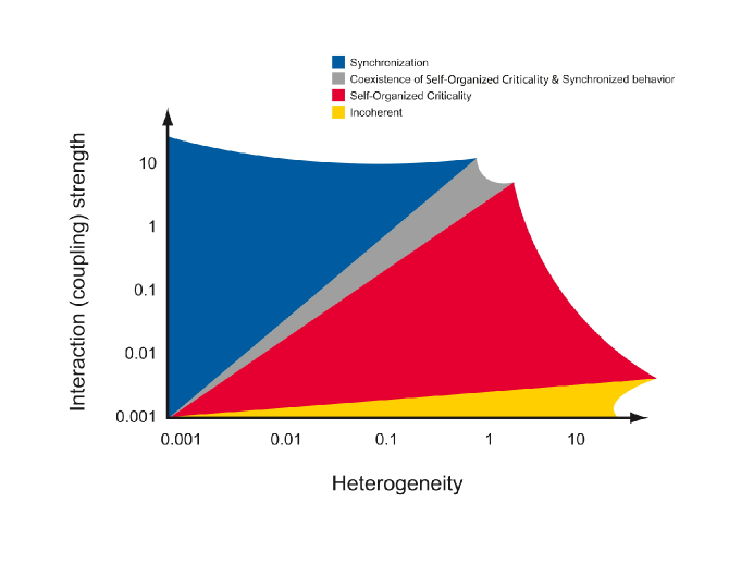
Figure 11: Qualitative phase diagram illustrating the effect of changes in coupling strength (y-axis) and heterogeneity (x-axis) on the behavior of systems (such as the brain) composed of interacting threshold oscillators. Marked increases in excitatory coupling drives the system towards the synchronized regime. Slight increases in coupling drive the system towards the power law regime indicative of self-organized criticality. Reproduced from Ref. [92], itself adapted from Ref. [145].

A generic qualitative phase diagram (Figure 11) depicts the main different regimes found in systems made of heterogeneous coupled threshold oscillators, such as sandpile models, Burridge-Knopoff block-spring models [120] and earthquake-fault models [144, 145, 20]: a power law regime (probably self-organized critical) (Figure 11, right lower half) is co-extensive with one of synchronization [153] with characteristic size events (Figure 11, upper left half). This phase diagram embodies the principal qualitative modes that result from the “competition” between strong coupling leading to coherence and weak coupling manifesting as incoherence. Coupling (or interaction strength) is dependent, among others, upon features such as the distance between constituent elements (synaptic gap size in the case of neurons), their type (excitatory or inhibitory) and extent of contact (number of synapses and their density), the existence and size of delays in the transmission of signals as well as their density and flux rate between constituent elements. Heterogeneity, the other determinant of the system s organization, may be present in the natural frequencies of the oscillators (when taken in isolation), in the distribution of the coupling strengths between pairs of oscillators, in the composition and structure of the substrate (earth or neuropil) and in their topology among others. As shown in Figure 11 for very weak coupling and large heterogeneity, the dynamics are incoherent; increasing the coupling strength (and/or decreasing the heterogeneity) leads to the emergence of intermediate coherence and of a power law regime (self-organized criticality (SOC)); further increases in coupling strength (and/or decreases in heterogeneity), force the system towards strong coherence/synchronization and periodic behavior.

The specific boundaries between these different regimes depend on the system under study and on the details of the constituting elements and their interactions. In addition, these boundaries may have multiple bifurcations across a hierarchy of partially synchronized regimes within the system. The diagram of Figure 11 is adapted from the study of a system of coupled fault elements subjected to a slow tectonic loading with quenched disorder in the rupture thresholds [145]. In the SOC regime, the extreme events are not different from smaller ones, making the former practically unpredictable or at most very weakly predictable [155]. In contrast, in the synchronized regime, the extreme events are different, i.e., they are outliers or “dragon-kings” [75, 137] occurring as a result of some additional amplifying mechanism; these outliers unlike those in the SOC regime, have a degree of predictability [133], as we discuss below.

The model described in section 1.7 constitutes a nice example of a system that can be described by the phase diagram shown in figure 11. The correspondence works as follows:

• The heterogeneity dimension corresponds to the amplitude of the noise $n$ defined in equation (9).

• The coupling strength is quantified by the ratio ${\chi\over\alpha}$ of the instability growth rate divided by the diffusive relaxation rate.

A large ratio ${\chi\over\alpha}$ corresponds to a large coupling strength because the local order parameter $S(r,t)$ then exhibits large fluctuations because the full amplitude between the two branches of the subcritical pitchfork bifurcation can be sampled, and these large fluctuations have proportionally a strong influence on neighboring locations. This rationalized the results that dragon-kings emerge only for relatively small noise levels $n$ and large ratios ${\chi\over\alpha}$.

3 Self-excited Hawkes process for epileptic seizures

The analogy with earthquakes and financial fluctuations, and in particular the evidence that seizures may trigger other seizures (inverse and direct Omori laws shown in figure 10), motivates the presentation of a class of stochastic processes that is specifically formulated to account for triggering, also called “self-excitation.” But, before diving in the formalism, some caveats and definitions must be addressed.

3.1 “Particles” versus “waves”

While clinical seizures are rather unambiguous objects on the basis of the often dramatic observable symptoms, continuous voltage recordings directly from the brains of human subjects (electrocorticogram, ECoG) show the existence of many so-called sub-clinical seizures [93, 90], i.e., ECoG patterns that are undistinguishable from their clinical siblings (except perhaps for their durations and extend of spread) but without obvious manifestations. In textbooks, “ictal” events are classified as having clinical manifestations and interictal events as lacking visible behavioral changes. not, in the usual sense of clinical manifestations. But the definition and characterization of relevant patterns that can be used for diagnosing incoming clinical seizures remains elusive. For instance, the above textbook concepts of “ictal” and “interictal” events turn out to be quite fuzzy, given the demonstration that their durations do not form two well-separated classes (long durations for ictal events and short duration for interictal events) but a continuum better characterized by scale-free power law statistics [91, 92]. In addition, so-called interictal events comprise additionally what have been coined as “spikes” and “bursts of spikes”. Figure 12 shows a trace of a continuous recording from the brain of a rat which received injections of a convulsant. One can observe at the top a pattern that qualifies as an epileptic seizure, followed by bursts of spikes or by single spikes. In some cases, interictal spikes appear to arise from a different location (in a given brain) from the site of seizure initiation, which has led some to propose that they are quite distinct mechanistically. As better recording methods are available and longer time series of ECoG provide data for more sophisticated statistical analyses, understanding the relationship between spikes, bursts and seizures is highly relevant, given the growing realization of the fuzziness of past classifications based mainly on clinical criteria. Moreover, one should not exclude the possibility that spikes and bursts could be relevant diagnostics or even precursory signals announcing clinical seizures, since they also constitute signatures of the excitatory activity of the brain.

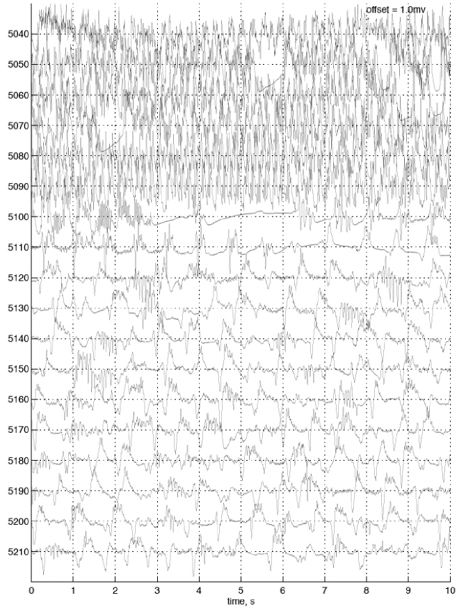
Figure 12: Continuous voltage recorded directly from the brain of a rat which received injections of an epileptogenetic substance.

In the following, we formulate a model of self-excitation that remains as general as possible, keeping open the possibility for interactions between spikes, bursts and seizures. Similarly to earthquakes or financial crashes, the key idea is to view the activity of a brain, as measured by electrocorticograms, as a wave-like background on which particle-like structures appear and possibly interact. We refer to this view as the “particle” approach, as opposed to the “wave” approach. The “wave” approach consists in viewing the ECoG as a continuous signal and then apply various signal analysis techniques, for instance derived from the theory of dynamical systems and chaos [82]. In contrast, the “particle” approach assumes that coherent structures or patterns exist on the noisy “wave” background, allowing to treat them as individuals or events. The formalism is then constructed to describe the relationships between these discrete events.

3.2 Brief classification of point processes

When using the “particle” point of view, the relevant mathematical language is that of so-called point processes (also known as shot-noise in physics or jump processes in finance). Daley and Vere-Jones provide a rigorous development of the theory of point processes [22].

The (conditional) rate $\lambda(t|H_{t})$ (also called “conditional intensity”) of a point process is defined by

$$\lambda(t|H_{t})={\rm lim}_{\Delta\to 0}~{}~{}{1\over\Delta}{\rm Pr}({\rm event~{}occurs~{}in}~{}[t,t+\Delta]|H_{t})~{},$$ (14)

where Pr$(X)$ means “probability that event $X$ occurs.” The symbol $H_{t}$ represents the entire history up to time $t$, which includes all previous events. This definition is straightforward to generalize for space-dependent intensities $\lambda(t,{\vec{t}}|H_{t})$ and to include marks such as amplitudes or magnitudes (see below). The Poisson process is the special case such that $\lambda(t|H_{t})$ is constant. Recall that the simplest point process is the memoryless Poisson process, in which events occur continuously and independently of one another. The term “conditional” refers to the fact that, in general, the rate $\lambda(t|H_{t})$ is not constant but may depend on the past history, i.e., on the specific realization of past events.

Let us define $f(t|H_{t})$ as the probability density function (pdf) time until the next event (possibly dependent on more than just the last event, when the process in non-Markovian) and $F(t|H_{t})$ as the corresponding survivor function (or complementary cumulative distribution function). The relationship between the conditional intensity and these two quantities is given by

$$\lambda(t|H_{t})={f(t|H_{t})\over F(t|H_{t})}~{}.$$ (15)

The probability of an event in the time interval $[t_{c},t_{c}+s]$ is given by

$$P(t_{c};s|H_{t_{c}})=1-\exp\left(-\int_{t_{c}}^{t_{c}+s}\lambda(u|H_{t_{c}})du\right)~{}.$$ (16)

When an event occurs, the history $H_{t}$ changes and therefore $\lambda(t|H_{t})$ may change abruptly, as it is defined as a piecewise continuous function between events. Another useful relationship relates the pdf $f(t_{i}|H_{t})$ for the $i$-th event to the conditional density, by differentiation of equation (16):

$$f(t_{i}|H_{t_{i}})=\lambda(t_{i}|H_{t_{i}})\exp\left(-\int_{t_{i-1}}^{t_{i}}\lambda(u|H_{u})du\right)~{}{\cal I}(t_{i}-t_{i-1})~{},$$ (17)

where ${\cal I}(\cdot)$ is the Heaviside step function.

$\bullet$ Renewal processes: Renewal processes constitute the simplest class of point processes. A renewal process is a particular class of temporal point process in which the probability of occurrence of the next event depends only on the time since the last event. The pdf of the waiting time from the $(i-1)$-th event to the $i$-th one is defined by

$$f(t_{i}|H_{t_{i}}=f(t_{i}|t_{i-1})=f(t_{i}-t_{i-1})~{}{\cal I}(t_{i}-t_{i-1})~{},$$ (18)

expressing the fact that the history $H_{t_{i}}$ is reduced to the knowledge of $t_{i-1}$. Renewal processes are to point processes what are Markov processes to general stochastic processes.

One can equivalently defined renewal processes by the fact that their conditional intensity at time $t>t_{i}$, where $i$ is the index of the last event, depends only on the occurrence time of the last event $t_{i}$:

$$\lambda(t_{i}|H_{t_{i}})=\lambda(t-t_{i})~{}.$$ (19)

The Poisson process is the simplest renewal process, and corresponds to the specification

$$f_{\rm Poisson}(\tau;\lambda)=\lambda\exp(-\lambda\tau)~{},$$ (20)

where we note $\tau=t-t_{i}$, the running time since the last event $i$. This exponential form of the Poisson process is uniquely associated with its memoryless property, which can be quantified by asking for instance “what is the average remaining waiting time at present time $t$, given that a time $t-t_{i}$ has passed since the last event?” It turns out that the Poisson process is the only process such that the average remaining time remains equal to $1/\lambda$ at all times $t$. The conditional distribution of the remaining time, conditional on having already waiting the time $t-t_{i}$ since the last event also remains unchanged in the form (20). Sornette and Knopoff have offered a systematic classification of renewal processes into three classes [142].

1. When the pdf $f(\tau)$ has a tail decaying faster than exponential, the longer the time since the last event, the shorter the average remaining waiting time till the next event.

2. When the pdf $f(\tau)$ has an exponential tail, the average remaining waiting time till the next event is independent of the time that has elapsed since the last event (this is the Poisson process).

3. When the pdf $f(\tau)$ has a tail decaying slower than exponential, the longer the time since the last event, the longer the average remaining waiting time till the next event.

These statements can be made more precise by calculating explicitly the full shape of the conditional distribution of waiting time till the next event, conditional on having already waiting some time $t-t_{i}$ since the last event that occurred at $t_{i}$. See Ref. [142] for detailed information. Osorio et al. have used this statistics as one of the diagnostics to characterize the sequence of epileptic seizures and to compare with earthquake sequences [91, 92].

$\bullet$ Clustering models: These models capture the general observation for earthquakes, financial volatility and seizures that they occur in bursts, that is, according to patterns exhibiting much more clustering or grouping than predicted by renewal processes.

Clustering models are usually constructed from two processes: a cluster center process, which is often a renewal process, and a cluster member process. In simple terms, the center events are main events or sources, from which the member events derive. The cluster member process consists of events that are triggered by the cluster centers via a triggering function $h(t-t_{i},\xi)$, which usually depends only on the time $t-t_{i}$ since the occurrence time $t_{i}$ of the cluster center, and on a stochastic amplitude $\chi$ drawn from a distribution usually chosen to be invariant in time. In other words, cluster centers are parents and the cluster members are their corresponding offsprings: a given parent triggers only his cohort of offsprings and has no influence on the offsprings of other parents (center sources).

An example is given by the simple aftershock model, which considers that there are main shocks distinctly different from their aftershocks. The former are the cause of the later, which cluster strongly after them. Such aftershock model is the standard textbook model for main earthquakes and their aftershocks. It consists in writing the conditional intensity as

$$\lambda(t|H_{t}^{c},\Theta)=\lambda_{c}+\sum_{i_{c}|t_{i_{c}}<t}h(t-t_{i},\xi)~{},$$ (21)

where $H_{t}^{c}$ is the history up to time $t$ that needs only include information about the cluster centers $\{t_{i_{c}},\chi_{i_{c}}\}_{1\leq i_{c}\leq N}$, as cluster members do not trigger their own events and do not influence the future. In the specification (21), we have assumed for simplicity that the cluster center process is a Poisson process with constant rate $\lambda_{c}$. The triggering process from centers to members is described by the set of parameters $\Theta$ characterizing the kernel $h(t-t_{i},\xi)$ quantifying the ability of centers to trigger their offsprings.

$\bullet$ Self-excited models: These models were first introduced by Hawkes [44, 43] and Hawkes and Oakes [45]. They generalize the cluster models by allowing each event, including cluster members, i.e., aftershocks, to trigger their own events according to some memory kernel $h(t-t_{i},\xi)$.

$$\lambda(t|H_{t},\Theta)=\lambda_{c}+\sum_{i|t_{i}<t}h(t-t_{i},\xi)~{},$$ (22)

where the history $H_{t}=\{t_{i}\}_{1\leq i\leq N}$ now includes all events and the sum in expression (22) runs over all triggered events. The term $\lambda_{c}$ means that there are still external background sources occurring according to a Poisson process with constant intensity $\lambda_{c}$ but all other events can be both triggered by previous events and can themselves trigger their offsprings. This gives rise to the existence of many generations of events.

$\bullet$ Marked self-excited point processes: This class is a multidimensional extension of the former self-excited process. The generalization consists in associating with each event some marks (possible multiple traits), drawn from some distribution $p(m)$, usually chosen invariant as a function of time:

$$\lambda(t,m|H_{t},\Theta)=p(m)\left(\lambda_{c}+\sum_{i|t_{i}<t}h(t-t_{i},\xi,m_{i})\right)~{},$$ (23)

where the mark $m_{i}$ of a given previous event now controls the shape and properties of the triggering kernel describing the future offsprings of that event $i$. The history now consists in the set of occurrence times of each triggered event and their marks: $H_{t}=\{t_{i},m_{i}\}_{1\leq i\leq N}$. The first factor $p(m)$ in the r.h.s. of expression (23) writes that the marks of triggered events are drawn from the distribution $p(m)$, independently of their generation and waiting times. This is a simplifying specification, which can be relaxed. Inclusion of spatial kernel to describe how distance impacts triggering efficiency is straightforward.

A particularly well-studied specification of this class of marked self-excited point process is the so-called Epidemic-Type-Aftershock-Sequence (ETAS) model [67, 85]:

$$\lambda(t,m|H_{t},\Theta)=p(m)\left(\lambda_{c}+\sum_{i|t_{i}<t}{ke^{a(m_{i}-m_{0})}\over(t-t_{i}+c)^{1+\theta}}\right)~{},$$ (24)

where $p(m)$ is given by the Gutenberg-Richter law with exponent $\beta$ discussed already in section 2.2. The memory kernel is chosen as the power law (called the Omori law) with exponent $1+\theta$. The lower magnitude cut-off $m_{0}$ is such that events with marks smaller than $m_{0}$ do not generate offsprings. This is necessary to make the theory convergent and well-defined, otherwise the crowd of small events may actually dominate. The time constant $c$ ensures normalization and finiteness of the triggering rate immediately following any event. Each event (of magnitude $m$) triggers other events with a rate $\sim e^{am}$, which defines the so-called fertility or productivity law. The set of parameters is $\Theta=\{\beta,\lambda_{c},k,a,m_{0},c,\theta\}$. Figure 13 shows a typical realization of a sequence of events generated with the ETAS model.

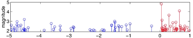
Figure 13: Typical realization of a sequence of events using the ETAS model. The horizontal axis is time and the vertical axis shows the magnitude $m$ (or mark) of each event.

An observed “aftershock” sequence in the ETAS model is the sum of a cascade of events in which each event can trigger more events. The triggering process may be caused by various mechanisms that either compete with each other or combine. The ETAS model is parsimonious as it lumps all the complications of physical and biological properties as well as geometric structural geometry in a few key parameters quantifying the Omori law, the Gutenberg-Richter law and the productivity law. This is particularly important as seismic as well as seizure data is relatively sparse, has limited precision accuracy, and the characterization of the properties of these dynamical processes is bound to be full of misleading paths if solid theoretical and analytical guidelines do not constrain the research on empirical data.

This class of marked self-excited point processes is now considered as the benchmark that best describes the statistical properties of spatio-temporal earthquake catalogs. In particular, the textbook classification of foreshocks, mainshocks and aftershocks is now considered obsolete by many seismologists, due to the cumulative evidence that any earthquake may trigger other earthquakes through a variety of physical mechanisms but this does not allow one to put a tag on them [26]. The textbook classification of foreshocks, mainshocks and aftershocks is essentially a human-made construction that is open to revision as a function of the development of the sequences of earthquake magnitudes. For instance, if an aftershock happens to have a larger magnitude that the earthquake that was qualified previously as a mainshock, it is reclassified as the new mainshock of the unfolding sequence and the previous mainshock becomes one of its foreshock. The fact that many small earthquakes occur after large mainshocks, and are thus classified as aftershocks, is simply due to the fact that large earthquakes trigger many earthquakes and most earthquakes are small. Thus, it is improbable (but not impossible) that a large earthquake is followed in close succession by still larger earthquakes.

Rather than keeping the textbook classification that foreshocks are precursors of mainshocks and mainshocks trigger aftershocks, the self-excited class of models starts from the hypothesis that a parsimonious description of seismicity does not require the division between foreshocks, mainshocks and aftershocks that are indistinguishable from the point of view of their physical processes [26, 25] (it is however sometimes convenient to use the time-honored foreshocks-mainshocks-aftershocks terminology, as long as it is understood that the model refers only to events which may trigger other earthquakes). But the story is not written as, recently, some evidence of a difference between spontaneous and triggered earthquakes was obtained [165].

We propose that a similar approach may be a useful starting point in epileptology. Single epileptiform discharges (spikes), bursts of spikes and seizures may not be, as often claimed, distinct phenomena but simply reflect the heterogeneous manifestations of processes governed by the same mechanisms or laws while having a self-triggering capacity or degree of “fertility.” This seemingly radical shift in conceptualization may provide a deeper and more fruitful insight into the dynamics of ictiogenesis.

The ETAS model and other related models developed on similar principles are popular with statisticians interested in the characterizations of complex spatio-temporal patterns (in particular with applications to seismicity) [68, 83, 102, 86, 14, 166, 15, 88, 87, 167], using maximum likelihood methods for parameter estimations and residual analysis [87, 88] for the detection of deviations from normal seismicity. We believe that these statistical techniques could be usefully applied to seizure time series.

A detailed understanding of the observable properties of the marked self-excited point processes has been developed in the last decade, that we briefly summarize below.

3.3 Main properties of the ETAS model

We stress that the advantage of the ETAS model is to offer a very parsimonious description of the complex spatio-temporal organization of systems characterized by self-excitation of “bursty” events, without the need to invoke ingredients other than the well-documented stylized facts reported above: distribution of event sizes, Omori law and productivity law. An important insight is that the Omori law may come in different forms, which can be derived from the same model only via the change of a crucial parameter, the branching ratio $n$. The parameter $n$ is defined as the mean number of events of first generation triggered per event. Using the notation of expression (24), the branching ratio is given by

$$n=K{\beta\over\beta-a}~{},~{}~{}~{}~{}~{}~{}{\rm where}~{}K:={k\over\theta c^{\theta}}~{}.$$ (25)

The variability of the apparent Omori’s exponent $p$ is then obtained as a result of the relative importance of cascades of aftershocks, of aftershocks of aftershocks, and so on over possibly many generations [80]. The branching ratio $n$ can vary with time and from location to location. In the context of epileptic seizures, it can be used as a diagnostic of the susceptibility of the brain to trigger epileptic seizures.

While the results summarized below pertain to earthquakes, the method used to obtain them can be applied to seizure time series as well as financial fluctuations (for an early attempt in this later domain, see Ref. [13]).

3.3.1 Subcritical, critical and supercritical regimes

Precise analytical results and numerical simulations show the existence of three time-dependent regimes, depending on the “branching ratio” $n$ and on the sign of $\theta$. This classification is valid for the range of parameters $a<\beta$. When the productivity exponent $a$ is larger than the exponent $\beta$ of the Gutenberg-Richter law, an explosive regime occurs leading to stochastic finite-time singularities [140], a regime that we do not consider further below, but which is relevant to describe the accelerated damage processes leading to global systemic failures in possibly many different types of systems [133].

1. For $n<1$ (sub-critical regime), the rate of events triggered by a given shock decays according to an effective Omori power law, characterized by a crossover from an Omori exponent $p=1-\theta$ for $t<t^{*}$ to a larger exponent $p=1+\theta$ for $t>t^{*}$ [128, 51], where $t^{*}$ is a characteristic time $t^{*}\sim c/(1-n)^{1/\theta}$, which is controlled by the distance from $n$ to $1$.

2. For $n>1$ and $\theta>0$ (super-critical regime), one finds a transition from an Omori decay law with exponent $p=1-\theta$ at early times since the mainshock to an explosive exponential increase of the seismicity rate [128, 51, 114].

3. In the case $\theta<0$, there is a transition from an Omori law with exponent $1-|\theta|$ similar to the local law, to an exponential increase at large times, with a crossover time $\tau$ different from the characteristic time $t^{*}$ found in the case $\theta>0$.

These results may open the road for the discovery of new types of seizure precursors. These could include (i) variable $p$-values, in particular the suggestion that a small $p$-value may be a precursor of a large event, (ii) relative seizure quiescence in some spatial domain preceding the occurrence of large seizures, (iii) exponential increase in seizure activity in some other spatial domains preceding large events.

3.3.2 Importance of small events for triggering other events of any size [46, 47]

In the context of earthquakes for which the productivity exponent $a$ is estimated smaller than, but close to, the Gutenberg-Richter exponent $\beta$, small events have been found to provide a dominating contribution to the overall activity, as their number more than compensates their relatively smaller individual impact. This is due to the structure of the model in which all events can trigger other events. This realization comes as a big surprise to experts, who have been accustomed to the concept that only large and great earthquakes needed to be considered since they overwhelmingly dominate the overall release of energy in the Earth crust. But not so, for the triggering ability, as is now understood. Can there be a similar situation for epileptic seizures, for whom the myriad single spikes, bursts of spikes and subclinical seizures play an important role in the triggering of clinical seizures?

3.3.3 Effects of undetected seismicity: constraints on the size of the smallest triggering event from the ETAS model [151]

The mechanism of event triggering together with simple assumptions of self-similarity, as captured in the simple ETAS specification, make obligatory the existence of a minimum magnitude $m_{0}$ below which events do not or only weakly trigger other events. It turns out to be possible to estimate an order of magnitude of $m_{0}$ by noting that the magnitude $m_{d}$ of completeness of empirical catalogs has no reason to be the same as $m_{0}$, and by using diverse empirical data based on maximum likelihood inversions of observed aftershock sequences of real catalogs with the ETAS model. The obtained constraint $m_{0}\simeq-1\pm 2$ is loose and reflects the many uncertainties in the model calibrations and model errors.

3.3.4 Apparent earthquake sources and clustering biased by undetected seismicity [150, 110]

In models of triggered-seismicity, the detection threshold $m_{d}$ is commonly equated to the magnitude $m_{0}$ of the smallest triggering earthquake. This unjustified assumption neglects the possibility that shocks below the detection threshold may trigger observable events. Distinguishing between the detection threshold $m_{d}$ and the minimum triggering earthquake $m_{0}\leq m_{d}$, and considering the branching structure of one complete cascade of triggered events, an apparent branching ratio $n_{a}$ and an apparent background source $S_{a}$ can be determined from the exact calculation of the sequence of observed triggered events with marks above the detection threshold $m_{d}$. The presence of smaller undetected events that are capable of triggering larger events is the cause for the renormalization. One could imagine that triggering between seizures could be similarly renormalized when not taking into account of structures such as spikes and bursts of spikes if the later have some triggering effects on seizures.

3.3.5 Cascades of triggered events

By comparison between synthetic catalogs generated with the ETAS model and real seismicity, it is now understood that a surprisingly large fraction of earthquakes in real seismicity are probably triggered by previous events. Recent conservative lower bounds suggest that at least $60\%$, and perhaps up to $99\%$ of earthquakes are triggered by previous earthquakes [53, 151, 150, 80]. This fraction is nothing but the so-called average branching ratio $n$ or mean number of triggered event per earthquake, averaged over all magnitudes [53]. In addition, within the picture that earthquakes can trigger events which themselves trigger new events and so on according to the same basic physics, then, most triggered events within a sequence should be triggered indirectly through cascades [53]. Therefore, previous observations that a significant fraction of earthquakes are triggered earthquakes imply that most aftershocks are indirectly triggered by the mainshocks. In the class of ETAS models, this has the implication that the observed Omori law is obtained from a renormalization of the direct Omori law (describing the direct interactions between triggering and triggered earthquakes) to the global law with different exponent $p$ [128, 51]. The cascades of secondary triggering provides a mechanism for slow aftershock sub-diffusion [50, 49] and slow foreshock migration [56, 52].

3.3.6 Other results available for marked self-excited point processes

A number of other interesting mathematical and statistical results have been derived for the ETAS model, which show that the model has non standard properties resulting from the interplay between the triggered cascades and the two power laws characterizing the distribution of sizes and the productivity process. These results have been obtained by rigorous mathematical derivations using probability generating functions:

• non-mean field anomalous exponents for the distribution of “cluster” sizes due to the interplay between cascades of generation and the power laws of productivity and of marks (magnitudes) [106];

• non-mean field distributions of lifetimes and total number of generations before extinctions of aftershock sequences emanating from isolated main shocks [108];

• the distribution of waiting times between events in a given region is characterized by an approximate power law [111, 113, 149];

• stochastic reconstruction of the genealogy of the cascades of triggered events [166, 167, 80, 148].

3.4 Forecasts using self-excited marked point processes

The understanding of the importance of cascades of triggered seismicity has led to important improvements of existing methods of earthquake forecasts [71], based on variations of the ETAS model, by taking into account the cascades of secondary triggering [54, 48, 157].

As a quantitative theoretical check, the number $r$ of earthquakes in finite space-time windows is often taken as the target for forecasts: for instance within the RELM (Regional Earthquake Likelihood Models: www.relm.org) project in Southern California, a forecast is expressed as a vector of earthquake rates specified for each multi-dimensional bin [122], where a bin is defined by an interval of location, time, magnitude and focal mechanism and the resolution of a model corresponds to the bin sizes. The full theory of this observable within the ETAS model has been developed using the formalism of generating probability functions (GPF) describing the space-time organization of earthquake sequences [109, 112]. The calibration of the theory to the empirical observations for the California catalog shows that it is essential to augment the ETAS model by taking account of the pre-existing frozen heterogeneity of spontaneous earthquake sources. This seems natural in view of the complex multi-scale nature of fault networks, on which earthquakes nucleate. The extended theory is able to account for the empirical observation satisfactorily. In particular, the probability density functions $P_{\rm data}(r)$ of the number $r$ of earthquakes in finite space-time windows for the California catalog, over fixed spatial boxes $5\times 5$ km², $20\times 20$ km² and $50\times 50$ km² and time intervals $dt=1,~{}10,~{}100$ and $1000$ days have been determined. One finds a stable power law tail compatible with $P_{\rm data}(r)\sim 1/r^{1+(b/\alpha)}$ [109, 112]. This result recovers previous estimates with different statistical methods and for large space and time windows [17, 81, 118], while proposing a simple and generic explanation in terms of cascades of triggering of earthquakes. This example and others [55] show the power of the simple concept of triggered seismicity to account for many (most?) empirical observations.

The Working Group on Regional Earthquake Likelihood Models (RELM) has invited long-term (5-year) forecasts for California in a specific format to facilitate comparative testing [27, 28, 123, 121, 124]. Building on RELM’s success, the Collaboratory for the Study of Earthquake Predictability (CSEP, www.cseptesting.org) inherited and expanded RELM’s mission to regionally and globally test prospective forecasts [124, 163, 159]. Many of the competing models are based on concept of earthquake triggering embodied in the marked self-excited conditional point processes.

New developments for point processes include the adaptation of data assimilation methods [158]. Recall that, in meteorology, engineering and computer sciences, data assimilation is routinely employed as the optimal way to combine noisy observations with prior model information for obtaining better estimates of a state, and thus better forecasts, than can be achieved by ignoring data uncertainties. Earthquake forecasting as well as seizure prediction, too, suffer from measurement errors and from model information that is limited, and may thus gain significantly from data assimilation. Werner et al. have presented perhaps the first fully implementable data assimilation method for forecasts generated by a point-process model [158]. The method has been tested on a synthetic and pedagogical example of a renewal process observed in noise, which is relevant to the seismic gap hypothesis, models of characteristic earthquakes and to recurrence statistics of large quakes inferred from paleoseismic data records. In order to address the non-Gaussian statistics of earthquakes, it was necessary to use sequential Monte Carlo methods, which provide a set of flexible simulation-based methods for recursively estimating arbitrary posterior distributions. Extensive numerical simulations have demonstrated the feasibility and benefits of forecasting earthquakes based on data assimilation. The forecasts based on the Optimal Sampling Importance Resampling (OSIR) particle filter are found significantly better than those of a benchmark forecast that ignores uncertainties in the observed event times. We predict that data assimilation will also become an important tool for seizure predictions in the future.

3.5 A preliminary attempt to generate synthetic ECoG with the ETAS model

The following is a modest example of how to generate synthetic time series that look like electrocorticogram (ECoG) using the ETAS model defined by the conditional intensity given by expression (24). We imagine that the elementary events are “spikes” and that spikes can excite other spikes following the ETAS specification. Sequences of closely occurring spikes may then define bursts and seizures can perhaps be observed when bursts are sufficiently clustered.

The synthetic ECoG are generated as follows. For a given choice of the parameter set $\Theta=\{\lambda_{c},\beta,n,a,m_{0},c,\theta\}$, we generate a time series of events $\{t_{i},m_{i}\}$, in which each event $i$ is characterized by its occurrence time $t_{i}$ and its mark $m_{i}$. Note that we use $n$ instead of $k$, but the two are related directly through expression (25).

Then, we assume that each event $i$ is associated with a “spike pattern” in a virtual ECoG recording given by

$$F(t-t_{i})={\rm sign}_{i}\cdot f_{i}\cdot{1\over\sqrt{2\pi}\tau_{i}^{3}}(t-t_{i})\exp\left(-{(t-t_{i})^{2}\over 2\tau_{i}^{2}}\right)~{},$$ (26)

where

$$f_{i}=f_{0}\cdot 10^{\alpha m_{i}}~{},~{}~{}~{}~{}~{}~{}~{}\tau_{i}=\tau_{0}\cdot 10^{dm_{i}}~{}.$$ (27)

The signal $F(t-t_{i})$ is thus a derivative of a Gaussian function and shows a typical dipole structure with a positive arch followed by a negative arch or vice-versa, depending on the sign term ‘${\rm sign}_{i}$’ that is chosen here at random and independently for each event. The mark $m_{i}$ of event $i$ is assumed to control the amplitude $f_{i}$ of the spike and its duration $\tau_{i}$ according to the expressions (27).

Figure 14: Synthetic electrocorticogram constructed with the ETAS model and using the spike pattern given by expression (26) with (27) for the following parameters: $\{\lambda_{c}=1,\beta=2/3,n=0.5,a=0.2,m_{0},c=60,\theta=0.5,a=0.001,d=0.001\}$.

Figures 14 and 15 show two realizations with the same parameters, except for the memory exponent $\theta=0.5$ in the former and $\theta=0.05$ in the later. The comparison between the two figures illustrates the impact of the memory in the triggering of spikes by previous spikes. Figure 14 corresponds to a shorter lived memory and a more spiky regime, compared with figure 15.

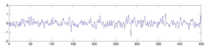
Figure 15: Synthetic electrocorticogram constructed with the ETAS model and using the spike pattern given by expression (26) with (27) for the following parameters: $\{\lambda_{c}=1,\beta=2/3,n=0.5,a=0.2,m_{0},c=60,\theta=0.05,a=0.001,d=0.001\}$.

Figure 16 shows a synthetic electrocorticogram obtained by changing the branching ratio from a low value $n=0.1$ to a large value $n=0.9$ abruptly in the middle of the graph. For $n=0.1$, the cumulative effect of ten spikes is needed on average to directly trigger an additional spike. For $n=0.9$, each spike triggers directly an additional spike almost by itself. This corresponds to a much more intense activity, with more correlations and burstiness. Seizure-like patterns can be obtained by decreasing $\lambda_{c}$ and increasing further the value of $n$ towards the critical value $1$.

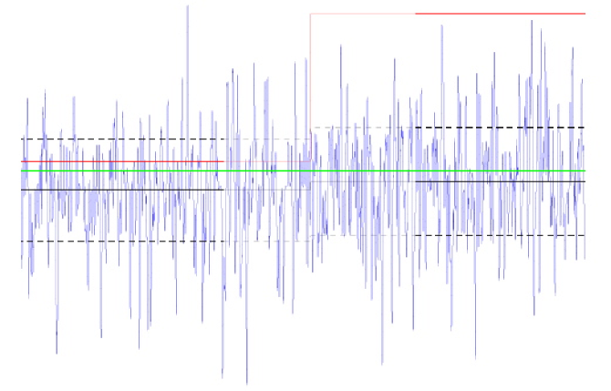
Figure 16: Synthetic electrocorticogram constructed with the ETAS model and using the spike pattern given by expression (26) with (27) for the following parameters: $\{\lambda_{c}=1,\beta=2/3,n=0.1\to 0.9,a=0.2,m_{0},c=60,\theta=0.05,a=0.001,d=0.001\}$.

4 Concluding remarks

The inherent value of predicting seizures has led to many efforts to fulfill this aim, efforts that to date have been unsuccessful. In particular, from our point of view, an acute limitation is the absence of understanding of the spatio- temporal behavior of seizures and the absence of corresponding models. While the reasons behind this state of affairs are multiple, there has been progress, if only in recognizing the challenges (after a first wave of over-optimism) as well as the need for rigorous testing procedures and for new approaches.

The task of predicting the occurrence of recurrent aperiodic events such as seizures would benefit from development of models that recognize the value of multi-scale approaches , aimed at excluding features that unnecessarily increase algorithmic complexity and the danger of computational irreducibility and its associated unpredictability. This chapter s central predicates are that seizures may be statistically predictable and that application of tools from statistical physics such as renormalization group theory may facilitate identification of the scale of observation (likely to be coarse-grained) that is the most informative. Through systematic quantitative comparisons with earthquakes, conceptual groundwork (neurons and faults are treated as coupled threshold oscillators of relaxation) is laid out that allows epileptology to adopt approaches with potential usefulness from the more mature fields of seismology and finance. Among those approaches briefly presented in this chapter, self-excited marked point processes are, in our opinion, worthy of investigation.

The perspectives we provide in this chapter and the approaches we propose are intended to stimulate new research directions to increase the knowledge of epilepsy dynamics and, with it, the likelihood of predicting seizures in a manner that improves quality of life of those to which they afflict.

5 Glossary

• The procedure that removes “uninformative” (for the task at hand) degrees of freedom to obtain a description of a system at a more integrated and computationally manageable level. Coarse-graining provides a range of techniques to bridge the “gap” between the microscopic and macroscopic levels.

• The meta-theory developed by L. Kadanoff, M. Fisher, K. Wilson and many others, which allows to construct macroscopic theories of critical phenomena at the macro-level, from the knowledge of constituents and interactions at the microscopic level.

• The phenomenon in which a change in a so-called “order parameter” causes a qualitative change (from one regime to another) in the systems’ dynamical behaviors. The theory of bifurcations has led to a classification of regime changes, which turn out to be reducible to a limited number of cases. The mathematical description of a bifurcation is called a normal form, which is a differential equation representing the time evolution of the order parameter, given the value(s) of the control parameter(s).

• A concept introduced in 1987 by P. Bak, C. Tang and K. Wiesenfeld, according to which many out-of-equilibrium dynamical spatio-temporal systems, which are slowly driven and which exhibit threshold-like responses, tend to self-organize to a dynamical state characterized by a broad range of avalanche sizes quantified by a power law distribution. A sub-class of self-organized critical systems can be shown to be made of systems functioning at or close to a standard critical point (in the sense of phase transitions in statistical physics). It is the non-standard type of slow driving of the “order parameters” that leads to the attraction of the dynamics to the usually unstable critical point.

• In the field of stochastic processes, one must distinguish between two broad classes: (i) Continuous or discrete time processes and (ii) point processes. An example of the former class is for instance the so-called random walk (or Wiener process in mathematical parlance). Point processes generate events that are distinct from “background” activity. In other words, the value of a point process is zero, except when “the event” occurs. In contrast, in the first class of processes, the activity is present at all time or occurs in continuing steps. Point processes, also called shot-noise in physics and jump processes in finance, are thus particularly suitable to describe and model system dynamics characterized by the occurrence of events, such as earthquakes, financial crashes and epileptic seizures.

References

- [1] Derek Abbott. Asymmetry and disorder: a decade of parrondo’s paradox. Fluct. Noise Lett., 9:129–156, 2010.
- [2] J.V. Andersen and D. Sornette. A mechanism for pockets of predictability in complex adaptive systems. Europhys. Lett., 70(5):697–703, 2005.
- [3] J.-C. Anifrani, C. Le Floc’h, D. Sornette, and B. Souillard. Universal log-periodic correction to renormalization group scaling for rupture stress prediction from acoustic emissions. J. Phys. I France, 5:631–638, 1995.
- [4] V. Arnol’d. Geometrical Methods in the Theory of Ordinary Differential Equations. 2nd ed., Springer, New York, 1988.
- [5] P. Bak. How Nature Works: the Science of Self-organized Criticality. Copernicus, New York, 1996.
- [6] A. Bellacicco, G. Koch, and A. ed. Vulpiani. Forecasting and Modelling for Chaotic and Stochastic Systems. Collana scientifica; 61, Collana scientifica (Franco Angeli editore), 1995.
- [7] P. Bird. An updated digital model of plate boundaries. Geochemistry, Geophysics, Geosystems, 4(3):1–52, 2003.
- [8] G. Boffetta, A. Celani, A. Crisanti, and A. Vulpiani. Predictability in two-dimensional decaying turbulence. Phys. Fluids, 9(3):724–734, 1997.
- [9] G. Boffetta, M. Cencini, M. Falcioni, and A. Vulpiani. Predictability: a way to characterize complexity. Physics Reports, 356:367–474, 2002.
- [10] D.D. Bowman, G. Ouillon, C.G. Sammis, A. Sornette, and D. Sornette. An observational test of the critical earthquake concept. J. Geophys. Res., 103:24359–24372, 1998.
- [11] G.J. Chaitin. Algorithmic Information Theory. Cambridge University Press, Cambridge, 1987.
- [12] D. Challet, M. Marsili, and Y.-C. Zhang. Minority Games: Interacting Agents in Financial Markets. Oxford Finance, Oxford University Press USA, 2005.
- [13] V. Chavez-Demoulin, Davison A.C., and A. C. McNeil. Estimating value-at-risk: a point process approach. Quantitative Finance, 5(2):227–234, 2005.
- [14] R. Console and M. Murru. A simple and testable model for earthquake clustering. J. Geophys. Res., 166:8699–8711, 2001.
- [15] R. Console, M. Murru, and A. M. Lombardi. Refining earthquake clustering models. J. Geophys. Res., 108(B10):2468, 2003.
- [16] A.C.C. Coolen. The Mathematical Theory of Minority Games: Statistical Mechanics of Interacting Agents. Oxford Finance, Oxford University Press USA, 2005.
- [17] A. Corral. Local distributions and rate fluctuations in a unified scaling law for earthquakes. Phys. Rev. E, 6803:5102, 2003.
- [18] R. Crane and D. Sornette. Robust dynamic classes revealed by measuring the response function of a social system. Proc. Nat. Acad. Sci. USA, 105(41):15649–15653, 2008.
- [19] M. C. Cross and P. C. Hohenberg. Pattern formation outside of equilibrium. Rev. Mod. Phys., 65:851–1112, 1993.
- [20] K. Dahmen, D. Ertas, and Y. Ben-Zion. Gutenberg-richter and characteristic earthquake behavior in simple mean-field models of heterogeneous faults. Phys. Rev. E., 58:1494–1501, 1998.
- [21] Vasilis Dakos, Marten Scheffer, Egbert H. van Nes, Victor Brovkin, Vladimir Petoukhov, and Hermann Held. Slowing down as an early warning signal for abrupt climate change. Proc. Natl. Acad. Sci. USA, 105(38):14308–14312, 2008.
- [22] D. J. Daley and D. Vere-Jones. An Introduction to the Theory of Point Processes, vol. I). Springer, New York, USA, 2003.
- [23] F. Deschatres and D. Sornette. The dynamics of book sales: Endogenous versus exogenous shocks in complex networks. Phys. Rev. E, 72:016112, 2005.
- [24] E. Edlund and M. Nilsson Jacobi. Renormalization of cellular automata and self-similarity. Journal of Statistical Physics, 139(6):972–984, 2010.
- [25] K.R. Felzer, R.E. Abercrombie, and G. Ekström. A common origin for aftershocks, foreshocks, and multiplets. Bull. Seismol. Soc. Am., 94:88–99, 2004.
- [26] K.R. Felzer, T. W. Becker, R.E. Abercrombie, G. Ekström, and J. R. Rice. Triggering of the 1999 mw 7.1 hector mine earthquake by aftershocks of the 1992 mw 7.3 landers earthquake. J. Geophys. Res., 107(B09):doi:10.1029/2001JB000911, 2002.
- [27] E. H. Field. Overview of the working group for the development of regional earthquake likelihood models (relm). Seismol. Res. Letts., 78(1):7–16, 2007.
- [28] E. H. Field. A summary of previous working groups on california earthquake probabilities. Bull. Seismol. Soc. Am., 97(4):1033–1053, 2007.
- [29] N. Fraysse, A. Sornette, and D. Sornette. Critical transitions made self-organized : proposed experiments. J.Phys.I France, 3:1377–1386, 1993.
- [30] U. Frisch. Turbulence: The Legacy of A. N. Kolmogorov. Cambridge University Press, 1996.
- [31] Sugihara G. and May R. Nonlinear forecasting as a way of distinguishing chaos from measurement error in time series. Nature, 344:734–741, 1990.
- [32] X. Gabaix, P. Gopikrishnan, V. Plerou, and H.E. Stanley. Institutional investors and stock market volatility. Q. J. of Econ., 121:461–504, 2006.
- [33] Luca Gammaitoni, Peter Hänggi, Peter Jung, and Fabio Marchesoni. Stochastic resonance. Rev. Mod. Phys., 70(1):223–287, Jan 1998.
- [34] A. Garcimartin, A. Guarino, L. Bellon, and S. Ciliberto. Statistical properties of fracture precursors. Phys. Rev. Lett., 79:3202–3205, 1997.
- [35] Robert J. Geller, David D. Jackson, Yan Y. Kagan, and Francesco Mulargia. Earthquakes cannot be predicted. Science, 275(5306):1616–1616, 1997.
- [36] L. Gil and D. Sornette. Landau-ginzburg theory of self-organized criticality. Phys. Rev.Lett., 76:3991–3994, 1996.
- [37] S. Gluzman and D. Sornette. Classification of possible finite-time singularities by functional renormalization. Physical Review E, 6601:016134, 2002.
- [38] P. Gopikrishnan, X. Gabaix, and H.E. Plerou, V. andStanley. Statistical properties of share volume traded in financial markets. Phys. Rev. E., 62:R4493–R4496, 2000.
- [39] O. Görnerup and M. Nilsson Jacobi. An algorithm for aggregating variables in linear dynamical systems. Advances in Complex Systems, 13(2):199–215, 2010.
- [40] P. Hagmann, L. Cammoun, X. Gigandet, R. Meuli, C.J. Honey, V.J. Wedeen, and O. Sporns. Mapping the Structural Core of Human Cerebral Cortex. PLoS Biol, 6(7):e159. doi:10.1371/journal.pbio.0060159, 2008.
- [41] James D. Hamilton. Time Series Analysis. Princeton University Press, 1994.
- [42] Peter Hänggi and Fabio Marchesoni. Artificial brownian motors: Controlling transport on the nanoscale. Rev. Mod. Phys., 81(1):387–442, Mar 2009.
- [43] A. G. Hawkes. Point spectra of some mutually exciting point processes. Royal Stat. Soc. Series B (Meth.), 33(3):438–443, 1971.
- [44] A. G. Hawkes. Spectra of some self-exciting and mutually exciting point processes. Biometrika, 58(1):83–90, 1971.
- [45] A. G. Hawkes and D. Oakes. A cluster process representation of a self-exciting process. J. of Appl. Prob., 11(3):493–503., 1974.
- [46] A. Helmstetter. Is earthquake triggering driven by small earthquakes? Phys. Res. Lett., 91:058501, 2003.
- [47] A. Helmstetter, Y.Y. Kagan, , and D. Jackson. Importance of small earthquakes for stress transfers and earthquake triggering. J. Geophys. Res., 110(B05S08):10.1029/2004JB003286, 2005.
- [48] A. Helmstetter, Y.Y. Kagan, and D.D. Jackson. Comparison of short-term and long-term earthquake forecast models for southern california. Bull. Seism. Soc. Am., 96:90–106, 2006.
- [49] A. Helmstetter, G. Ouillon, and D. Sornette. Are aftershocks of large californian earthquakes diffusing? J. Geophys. Res., 108(2483):10.1029/2003JB002503, 2003.
- [50] A. Helmstetter and D. Sornette. Diffusion of epicenters of earthquake aftershocks, omori’s law, and generalized continuous-time random walk models. Physical Review E, 6606:061104, 2002.
- [51] A. Helmstetter and D. Sornette. Sub-critical and supercritical regimes in epidemic models of earthquake aftershocks. J. Geophys. Res., 107(B10):2237, doi:10.1029/2001JB001580, 2002.
- [52] A. Helmstetter and D. Sornette. Foreshocks explained by cascades of triggered seismicity. J. Geophys. Res. (Solid Earth), 108(B10):10.1029/2003JB002409 01, 2003.
- [53] A. Helmstetter and D. Sornette. Importance of direct and indirect triggered seismicity in the etas model of seismicity. Geophys. Res. Lett., 30(11):doi:10.1029/2003GL017670, 2003.
- [54] A. Helmstetter and D. Sornette. Predictability in the etas model of interacting triggered seismicity. J. Geophys. Res. (Solid Earth), 108(2482):10.1029/2003JB002485, 2003.
- [55] A. Helmstetter and D. Sornette. Comment on “power-law time distribution of large earthquakes,’. Phys. Rev. Lett., 92:129801, 2004.
- [56] A. Helmstetter, D. Sornette, and J.-R. Grasso. Mainshocks are aftershocks of conditional foreshocks: How do foreshock statistical properties emerge from aftershock laws. J. Geophys. Res. (Solid Earth), 108(B10, 2046):doi:10.1029/2002JB001991, 2003.
- [57] W. Horsthemke and R. Lefever. Noise-Induced Transitions: Theory and Applications in Physics, Chemistry, and Biology. Springer Series in Synergetics, Springer, 1983.
- [58] K. Ide, P. Courtier, M. Ghil, , and A. Lorenc. Unified notation for data assimilation: Operational, sequential and variational. J. Meteor. Soc. Japan, 75:181–189, 1997.
- [59] K. Ide and D. Sornette. Oscillatory finite-time singularities in finance, population and rupture. Physica A, 307(1-2):63–106, 2002.
- [60] N. Israeli and N. Goldenfeld. Computational irreducibility and the predictability of complex physical systems. Phys. Rev. Letts., 92(7):074105, 2004.
- [61] N. Israeli and N. Goldenfeld. Coarse-graining of cellular automata, emergence, and the predictability of complex systems. Phys. Rev. E, 73:026203, 2006.
- [62] A. Johansen and D. D. Sornette. Finite-time singularity in the dynamics of the world population and economic indices. Physica A, 294(3-4):465–502, 2001.
- [63] A. Johansen and D. Sornette. Critical crashes. Risk, 12:91–94, 1999.
- [64] A. Johansen and D. Sornette. Critical ruptures. Eur. Phys. J. B, 18:163–181, 2000.
- [65] A. Johansen, D. Sornette, and O. Ledoit. Predicting financial crashes using discrete scale invariance. Journal of Risk, 1:5–32, 1999.
- [66] A. Johansen, D. Sornette, G. Wakita, U. Tsunogai, W.I. Newman, and H. Saleur. Discrete scaling in earthquake precursory phenomena: evidence in the kobe earthquake, japan. J. Phys. I France, 6:1391–1402, 1996.
- [67] Y. Y. Kagan and L. Knopoff. Stochastic synthesis of earthquake catalogs. J. Geophys. Res., 86:2853–2862, 1981.
- [68] Y.Y. Kagan. Likelihood analysis of earthquake catalogues. Geophys. J. Int., 106:135–148, 1991.
- [69] Y.Y. Kagan. Distribution of incremental static stress caused by earthquakes. Nonlinear Processes in Geophysics, 1:172–181, 1994.
- [70] Y.Y. Kagan. Observational evidence for earthquakes as a nonlinear dynamic process. Physica D, 77:160–192, 1994.
- [71] Y.Y. Kagan and D.D. Jackson. Probabilistic forecasting of earthquakes. Geophys. J. Int., 143:438–453, 2000.
- [72] Holger Kantz and Thomas Schreiber. Nonlinear Time Series Analysis. Cambridge University Press; 2 edition, 2004.
- [73] P.G. Kapiris, J. Polygiannakis, X. Li, X. Yao, and K.A. Eftaxias. Similarities in precursory features in seismic shocks and epileptic seizures. Europhys. Lett., 69:657–663, 2005.
- [74] Yurii A. Kravtsov and James B. Kadtke. Predictability of Complex Dynamical Systems. Springer Series in Synergetics, Springer, 1996.
- [75] J. Laherrere and D. Sornette. Stretched exponential distributions in nature and economy: “fat tails” with characteristic scales. Eur. Phys. J. B, 2:525–539, 1998.
- [76] M. Li and P. Vitanyi. An Introduction to Kolmogorov Complexity and its Applications. Springer-Verlag, New York, 1997.
- [77] F. Lillo and R.N. Mantegna. Power-law relaxation in a complex system: Omori law after a financial market crash. Phys. Rev. E, 68:016119, 2003.
- [78] E. N. Lorenz. Dimension of weather and climate attractors. Nature, 353:241–244, 1991.
- [79] V. Lyakhovsky, Y. Ben-Zion, and A. Agnon. Earthquake Cycle, Fault Zones and Seismicity Patterns in a Rheologically Layered Lithosphere. J. Geophys. Res., 106:4103–4120, 2001.
- [80] D. Marsan and O. Lengline. Extending earthquakes’ reach through cascading. Science, 319(5866):1076–1079, 2008.
- [81] M.S. Mega, P. Allegrini, P. Grigolini, V. Latora, L. Palatella, A. Rapisarda, and S. Vinciguerra. Power-law time distribution of large earthquakes. Phys. Rev. Lett., 90:188501, 2003.
- [82] Florian Mormann, Ralph G. Andrzejak, Christian E. Elger, and Klaus Lehnertz. Seizure prediction: the long and winding road. Brain, 130:314–333, 2007.
- [83] F. Musmeci and D. Vere-Jones. A space-time clustering model for historical earthquakes. Ann. Inst. Stat. Math., 44:1–11, 1992.
- [84] M. Nilsson Jacobi and O. Görnerup. A spectral method for aggregating variables in linear dynamical systems with application to cellular automata renormalization. Advances in Complex Systems, 12(2):1–25, 2009.
- [85] Y. Ogata. Statistical models for earthquake occurrence and residual analysis for point processes. J. Am. stat. Assoc., 83:9–27, 1988.
- [86] Y. Ogata. Space-time point process models for earthquake occurrences. Ann. Inst. stat. Mech., 50:379–402, 1998.
- [87] Y. Ogata. Space-time model for regional seismicity and detection of crustal stress changes. J. Geophys. Res., B03308:doi:10.1029/2003JB002621, 2004.
- [88] Y. Ogata, K. Katsura, and M. Tanemura. Modelling heterogeneous space-time occurrences of earthquake and its residual analysis. J. Roy. Statist. Soc. Ser. C, 52:499–509, 2003.
- [89] David Orrell. The Future of Everything: The Science of Prediction . Basic Books; 1st Thunder’s Mouth Press Ed., 2007.
- [90] I. Osorio, M.G. Frei, J. Giftakis, T. Peters, J. Ingram, M. Turnbull, M. Herzog, M. Rise, S. Schaffner, R. Wennberg, T. Walczak, M. Risinger, and C. Ajomone-Marsan. Performance re-assessment of a real-time seizure detection algorithm on long ecog series. Epilepsia, 43(12):1522–1535, 2002.
- [91] I. Osorio, M.G. Frei, D. Sornette, and J. Milton. Pharmaco-resistant seizures: Self-triggering capacity, scale-free properties and predictability? European Journal of Neuroscience, 30:1554–1558, 2009.
- [92] I. Osorio, M.G. Frei, D. Sornette, J. Milton, and Y.-C. Lai. Epileptic seizures, quakes of the brain. Phys. Rev. E., http://arxiv.org/abs/0712.3929, 2010.
- [93] I. Osorio, M.G. Frei, and S.B. Wilkinson. Real time automated detection and quantitative analysis of seizures and short term predictions of clinical onset. Epilepsia, 39(S16):615–627, 1998.
- [94] G. Ouillon, C. Castaing, and D. Sornette. Hierarchical scaling of faulting. J. Geophys. Res., 101(B3):5477–5487, 1996.
- [95] G. Ouillon and D. Sornette. Magnitude-dependent omori law: Theory and empirical study. J. Geophys. Res., 110:B04306, 2005.
- [96] J. Perello and J. Masoliver. Random diffusion and leverage effect in financial markets. Phys. Rev. E., 67:037102, 2003.
- [97] A. Pikovsky and J. Kurths. Coherence resonance in a noise-driven excitable system. Phys. Rev. Lett., 78:775–778, 1997.
- [98] V.F. Pisarenko and D. Sornette. On statistical methods of parameter estimation for deterministically chaotic time-series. Phys. Rev. E, 69:036122, 2004.
- [99] V.F. Pisarenko and D. Sornette. Properties of a simple bilinear stochastic model: estimation and predictability. Physica D, 237(4):429–445, 2008.
- [100] Robert. R. and C. Rosier. Long range predictability of atmospheric flows. Nonlinear Processes in Geophysics, 8:55–67, 2001.
- [101] A. Rapoport, D.A. Seale, I. Erev, and J.A. Sundali. Equilibrium play in large group market entry games. Management Science, 44(1):119–141, 1998.
- [102] S. L. Rathbun. Modelling marked spatio-temporal point patterns. Bull. Int. Stat. Inst., 55(Book 2):379–396, 1993.
- [103] G. Robinson and M. Thiel. Recurrences determine the dynamics. Chaos, 19:023104, 2009.
- [104] B.M. Roehner, D. Sornette, and J.V. Andersen. Response functions to critical shocks in social sciences: An empirical and numerical study. Int. J. Mod. Phys. C, 15(6):809–834, 2004.
- [105] J. Rundle, W. Klein, S. Gross, and D.L. Turcotte. Boltzmann fluctuations in numerical simulations of nonequilibrium lattice threshold systems. Phys. Rev. Lett., 75:1658–1661, 1995.
- [106] A. Saichev, A. Helmstetter, and D. Sornette. Anomalous scaling of offspring and generation numbers in branching processes. Pure and Applied Geophysics, 162:1113–1134, 2005.
- [107] A. Saichev, Y. Malevergne, and D. Sornette. Theory of Zipf’s law and beyond. Lecture Notes in Economics and Mathematical Systems, Vol. 632, Springer, 2009.
- [108] A. Saichev and D. Sornette. Anomalous power law distribution of total lifetimes of aftershock sequences. Phys. Rev. E, 70:046123, 2004.
- [109] A. Saichev and D. Sornette. Power law distribution of seismic rates: theory and data. Eur. Phys. J. B, 49:377–401, 2006.
- [110] A. Saichev and D. Sornette. Renormalization of the etas branching model of triggered seismicity from total to observable seismicity. Eur. Phys. J. B, 51(3):443–459, 2006.
- [111] A. Saichev and D. Sornette. “universal” distribution of inter-earthquake times explained. Phys. Rev. E, 97:078501, 2006.
- [112] A. Saichev and D. Sornette. Power law distribution of seismic rates. Tectonophysics, 431:7–13, 2007.
- [113] A. Saichev and D. Sornette. Theory of earthquake recurrence times. J. Geophys. Res., 112(B04313):doi:10.1029/2006JB004536, 2007.
- [114] A. Saichev and D. Sornette. Generation-by-generation dissection of the response function in long memory epidemic processes. European Physical Journal B, 75:343–355, 2009.
- [115] S.G. Sammis and D. Sornette. Positive feedback, memory and the predictability of earthquakes. Proc. Natl. Acad. Sci. USA, 99(SUPP1):2501–2508, 2002.
- [116] J.M. Sancho and J. García-Ojalvo. Noise-induced order in extended systems: a tutorial. Lecture Notes in Physics, 557:235–246, ed. J.A. Freund and T. Pöschel, Springer-Verlag, Berlin, 2000.
- [117] J. Satinover and D. Sornette. Taming manias: On the origins, inevitability, prediction and regulation of bubbles and crashes. chapter of the book “Governance and Control of Financial Systems: A Resilience Engineering Perspective”, Gunilla Sundström and Erik Hollnagel, eds., published by Ashgate Publishing Group in their Resilience Engineering Perspectives series, 2010.
- [118] N. Scafetta and B.J. West. Multiscaling comparative analysis of time series and a discussion on “earthquake conversations” in california. Phys. Rev. Lett., 92:138501, 2004.
- [119] Marten Scheffer, Jordi Bascompte, William A. Brock, Victor Brovkin, Stephen R. Carpenter, Vasilis Dakos, Hermann Held, Egbert H. van Nes, Max Rietkerk, and George Sugihara. Early-warning signals for critical transitions. Nature, 461:53–59, 2009.
- [120] J. Schmittbuhl, J.-P. Vilotte, , and S. Roux. Propagative macrodislocation modes in an earthquake fault model. Europhys. Lett., 21:375–380, 1993.
- [121] D. Schorlemmer and M. Gerstenberger. Relm testing center. Seismol. Res. Lett., 78(1):30, 2007.
- [122] D. Schorlemmer, M. Gerstenberger, S. Wiemer, and D. D. Jackson. Earthquake likelihood model testing. Seismological Research Letters, 78:17–29, 2007.
- [123] D. Schorlemmer, M. Gerstenberger, S. Wiemer, D. D. Jackson, and D. A. Rhoades. Earthquake likelihood model testing. Seismol. Res. Lett., 78(1):17, 2007.
- [124] D. Schorlemmer, J. D. Zechar, M. J. Werner, E. Field, D.D. Jackson, T. H. Jordan, and the RELM Working Group. First results of the regional earthquake likelihood models experiment. Pure and Appl. Geophys., 2009.
- [125] L. Smith. Chaos: A Very Short Introduction. Oxford University Press, USA, 2007.
- [126] R.J. Solomonoff. Algorithmic Probability: Theory and Applications, Information Theory and Statistical Learning. Springer N.Y., Emmert-Streib, F. and Dehmer, M. (Eds),, 2009.
- [127] A. Sornette, J. Dubois, J.L. Cheminée, and D. Sornette. Are sequences of volcanic eruptions deterministically chaotic? J. Geophys. Res., 96(B7):11931–11945, 1991.
- [128] A. Sornette and D. Sornette. Renormalization of earthquake aftershocks. Geophys. Res. Lett., 26:1981–1984, 1999.
- [129] D. Sornette. Self-organized criticality in plate tectonics. In Proceedings of NATO ASI “Spontaneous formation of space-time structures and criticality”, Geilo, Norway 2-12 april 1991, pages 57–106. edited by T. Riste and D. Sherrington, Kluwer Academic Press (Dordrecht, Boston), 1991.
- [130] D. Sornette. How to make critical phase transitions self-organized: a dynamical system feedback mechanism for self-organized criticality. J.Phys.I France, 2:2065–2073, 1992.
- [131] D. Sornette. Earthquakes: from chemical alteration to mechanical rupture. Physics Reports, 313(5):238–292, 1999.
- [132] D. Sornette. Mechanochemistry: an hypothesis for shallow earthquakes. In Earthquake thermodynamics and phase transformations in the Earth’s interior, pages 329–366. edited by R. Teisseyre and E. Majewski, International Geophysics Series, Vol. 76, Cambridge University Press (http://xxx.lanl.gov/abs/cond-mat/9807400), 2000.
- [133] D. Sornette. Predictability of catastrophic events: material rupture, earthquakes, turbulence, financial crashes and human birth. Proceedings of the National Academy of Sciences USA, 99(SUPP1):2522–2529, 2002.
- [134] D. Sornette. Why Stock Markets Crash (Critical Events in Complex Financial Systems). Princeton University Press, 2003.
- [135] D. Sornette. Endogenous versus exogenous origins of crises. In Extreme Events in Nature and Society, pages 329–366. eds. Albeverio, S., Jentsch, V. and Kantz, H., Springer, Berlin, pp 95-119, 2005.
- [136] D. Sornette. Critical Phenomena in Natural Sciences. 2nd ed., 2nd print, Springer Series in Synergetics, Springer, Heidelberg, 2006.
- [137] D. Sornette. Dragon-kings, black swans and the prediction of crises. International Journal of Terraspace Science and Engineering, 2(1):1–18 (http://arXiv.org/abs/0907.4290), 2009.
- [138] D. Sornette, D. Carbone, F. Ferré, C. Vauge, and E. Papiernik. Modèle mathématique de la parturition humaine: implications pour le diagnostic prenatal. Médecine/Science, 11:1150–1153, 1995.
- [139] D. Sornette, F. Ferré, and E. Papiernik. Mathematical model of human gestation and parturition: implications for early diagnostic of prematurity and post-maturity. Int. J. Bifurcation and Chaos, 4:693–699, 1994.
- [140] D. Sornette and A. Helmstetter. Occurrence of finite-time-singularity in epidemic models of rupture, earthquakes and starquakes. Physical Review Letters, 89(15):158501, 2002.
- [141] D. Sornette, A. Johansen, and J.-P. Bouchaud. Stock market crashes, precursors and replicas. J. Phys. I France, 6:167–175, 1996.
- [142] D. Sornette and L. Knopoff. The paradox of the expected time until the next earthquake. Bull. Seism. Soc. Am., 87(4):789–798, 1997.
- [143] D. Sornette, Y. Malevergne, and J.-F. Muzy. What causes crashes? Risk, 16(2):67–71 (http://arXiv.org/abs/cond–mat/0204626), 2003.
- [144] D. Sornette, P. Miltenberger, and C. Vanneste. Statistical physics of fault patterns self-organized by repeated earthquakes. Pure and Applied Geophysics, 142(3/4):491–527, 1994.
- [145] D. Sornette, P. Miltenberger, and C. Vanneste. Statistical physics of fault patterns self-organized by repeated earthquakes: synchronization versus self-organized criticality. In Recent Progresses in Statistical Mechanics and Quantum Field Theory, pages 329–366. Proceedings of the conference “Statistical Mechanics and Quantum Field Theory”, USC, Los Angeles, May 16-21, 1994, eds. P. Bouwknegt, P. Fendley, J. Minahan, D. Nemeschansky, K. Pilch, H. Saleur and N. Warner, World Scientific, Singapore, p. 313-332, 1995.
- [146] D. Sornette and V.F. Pisarenko. Fractal Plate Tectonics. Geophys. Res. Lett., 30(3):doi:10.1029/2002GL015043, 2003.
- [147] D. Sornette and C.G. Sammis. Complex critical exponents from renormalization group theory of earthquakes: Implications for earthquake predictions. J. Phys. I France, 5:607–619, 1995.
- [148] D. Sornette and S. Utkin. Limits of declustering methods for disentangling exogenous from endogenous events in time series with foreshocks, main shocks and aftershocks. Physical Review E, 79:061110, 2009.
- [149] D. Sornette, S. Utkin, and A. Saichev. Solution of the nonlinear theory and tests of earthquake recurrence times. Physical Review E, 77:066109, 2008.
- [150] D. Sornette and M.J. Werner. Apparent clustering and apparent background earthquakes biased by undetected seismicity. J. Geophys. Res., 110(B09303):doi:10.1029/2005JB003621, 2005.
- [151] D. Sornette and M.J. Werner. Constraints on the size of the smallest triggering earthquake from the etas model, baath’s law, and observed aftershock sequences. J. Geophys. Res., 110(B08304):doi:10.1029/2004JB003535, 2005.
- [152] R. S. Stein. Earthquake Conversations. Scientific American, 288(January issue):72–79, 2003.
- [153] S.H. Strogatz. Sync: How Order Emerges From Chaos In the Universe. Nature, and Daily Life (Hyperion), 2004.
- [154] H. Takayasu, H. Miura, T. Hirabayashi, and K. Hamada. Statistical properties of deterministic threshold elements: the case of market price. Physica A, 184(1-2):127–134, 1992.
- [155] N.N. Taleb. The Black Swan: The Impact of the Highly Improbable. Random House, New York, 2007.
- [156] R. Thom. Stabilité Structurelle et Morphogénèse. Benjamin, New York, 1972.
- [157] M.J. Werner, A. Helmstetter, D.D. Jackson, and Y.Y. Kagan. High resolution long- and short-term earthquake forecasts for california. Bull. Seismol. Soc. Am., November 20, 2009.
- [158] M.J. Werner, K. Ide, and D. Sornette. Earthquake forecasting based on data assimilation: Sequential monte carlo methods for renewal processes. Nonlinear Processes in Geophysics, http://arxiv.org/abs/0908.1516, 2010.
- [159] M.J. Werner, J.D. Zechar, W. Marzocchi, S. Wiemer, and the CSEP-Italy Working Group. Retrospective evaluation of the five-year and ten-year csep-italy earthquake forecasts. submitted 3 March 2010 to the CSEP-Italy special issue of the Annals of Geophysics, 2010.
- [160] K. G. Wilson. Problems in physics with many scales of length. Scientific American, 241(2):140–157, 1979.
- [161] S. Wolfram. Statistical mechanics of cellular automata. Rev. Mod. Phys., 55:601–644, 1983.
- [162] S. Wolfram. A New Kind of Science. Wolfram Media, 2002.
- [163] J. D. Zechar, D. Schorlemmer, M. Liukis, J. Yu, F. Euchner, P. J. Maechling, and T. H. Jordan. The collaboratory for the study of earthquake predictability: perspective on computational earthquake science. Concurrency and Computation: Practice and Experience, page doi:10.1002/cpe.1519, 2009.
- [164] X. Zhao and T. Chen. Type of self-organized criticality model based on neural networks. Phys. Rev. E, 65:026114, 2002.
- [165] J. Zhuang, J.A. Christophersen, M. K. Savage, D. Vere-Jones, Y. Ogata, and D. D. Jackson. Differences between spontaneous and triggered earthquakes: Their influences on foreshock probabilities. J. Geophys. Res., 113(B12):doi:10.1029/2008JB005579, 2008.
- [166] J. Zhuang, Y. Ogata, and D. Vere-Jones. Stochastic declustering of space-time earthquake occurrences. Journal of the American Statistical Association, 97:369–380, 2002.
- [167] J. Zhuang, Y. Ogata, and D. Vere-Jones. Analyzing earthquake clustering features by using stochastic reconstruction. J. Geophys. Res., 109(B5):B05301, doi:10.1029/2003JB002879, 2004.