On the Stability of Dust-Laden Protoplanetary Vortices

Abstract

The formation of planetesimals via gravitational instability of the dust layer in a protoplanetary disks demands that there be local patches where dust is concentrated by a factor of $\sim$ a few $\times 10^{3}$ over the background value. Vortices in protoplanetary disks may concentrate dust to these values allowing them to be the nurseries of planetesimals. The concentration of dust in the cores of vortices increases the dust-gas ratio of the core compared to the background disk, creating a ”heavy vortex.” In this work, we show that these vortices are subject to an instability which we have called the heavy-core instability. Using Floquet theory, we show that this instability occurs in elliptical protoplanetary vortices when the gas-dust density of the core of the vortex is heavier than the ambient gas-dust density by a few tens of percent. The heavy-core instability grows very rapidly, with a growth timescale of a few vortex rotation periods. While the nonlinear evolution of this instability remains unknown, it will likely increase the velocity dispersion of the dust layer in the vortex because instability sets in well before sufficient dust can gather to form a protoplanetary seed. This instability may thus preclude vortices from being sites of planetesimal formation.

1. Introduction

Current theories of planet formation postulate that dust grows from interstellar grain sizes ($\sim\mu m$) to $\sim\mathrm{km}$ size planetesimals in the disks observed around young stars. This process must proceed in stages: below $\sim$ cm scales, growth proceeds by ”sticky” grain-grain collisions. Above $\sim$ km scales, planetesimal growth proceeds by gravitational accretion. However, around meter scales, collisions between grains are destructive and another growth process is needed.

This process must be quick. The gaseous disk has a radial pressure gradient which partially supports it against gravity, leaving its rotation rate sub-Keplerian. The dust, meanwhile, sees no pressure gradient and therefore orbits at the Keplerian rate, leading to a headwind on the dust as it orbits in the gaseous disk. As a result, the dust rapidly spirals in to the star, at a rate

$$t\sim 200\left(\frac{r}{AU}\right)^{13/14}\mathrm{yr}$$ (1)

in the minimum mass solar nebula–far too short for the formation of planets (for a recent review, see Chiang & Youdin, 2009).

Gravitational instability in the dust layer is one mode by which planetesimals can grow at the m scale (Goldreich & Ward, 1973; Safronov, 1972). However, for this to proceed the dust density must be significantly enhanced by a factor of $\sim$ a few $\times 10^{3}$. The settling of dust to the midplane can enhance the dust density enormously, but when the dust density, $\rho_{\rm d}$ is similar to the gas density, $\rho_{\rm g}$, Kevin-Helmholtz instabilities limit further concentration (Weidenschilling & Cuzzi, 1993; Chiang, 2008; Barranco, 2009). Hence, the dust density enhancement is limited to $\sim 100$ for solar metallicity unless the metallicity of the gas is enhanced (see Youdin & Shu 2002) or the dust surface density is enhanced.

A natural way around these somewhat daunting timescale and surface density problems is to postulate the existence of regions in the disk where dust is significantly concentrated. This concentration may take place in persistent, large-scale vortices. On large enough scales (roughly $\gtrsim H$, where $H=c_{s}/\Omega$ is the scale height of the disk, $\Omega=\sqrt{GM_{*}/r^{3}}$ is the orbital frequency, $M_{*}$ is the mass of the star, $r$ is the radius, and $G$ is Newton’s constant), the dynamics of a thin disk ($H/r<<1$) become quasi-two dimensional. Such flows host inverse cascade processes in which energy flows to large scales, making the appearance of coherent, long-lived vortices a distinct possibility. Such large scale vortices could be seeded by the baroclinic instabilities (Lovelace et al., 1999; Varnière & Tagger, 2006; Lyra et al., 2009; Lesur & Papaloizou, 2009b), or by the quasi-2D decay of initial turbulence generated from the initial accretion flow from the pre-stellar envelope on to the disk (Bracco et al., 1999).

Previous studies, both analytic (Barge & Sommeria, 1995; Tanga et al., 1996; Chavanis, 2000) and computational (Bracco et al., 1999; Godon & Livio, 2000; Lyra et al., 2009), have demonstrated that anticyclonic vortices (those with vorticity antiparallel to the Keplerian rotation) effectively trap dust. As these vortices collect dust, the dust-to-gas ratio in the vortices increases. Hence, the gas in the vortices is denser than the gas in the surrounding disk. Can a density gradient between the vortex and surrounding gas or a density gradient within the vortex trigger new instabilities, destroying or modifying the vortex in the process? As we will show in this paper, the answer is yes: density gradients in vortices are destabilizing for vortices sufficiently heavy cores (and also for all vortices with light cores).

We note that this is not the only means by which dust can be concentrated into small regions of a protoplanetary disk. Youdin & Goodman (2005) have shown that the (inward) radial migration of dust in a gaseous disk is subject to a gas-dust streaming instability. The nonlinear evolution of this streaming instability leads to large concentrations of dust (Youdin & Johansen, 2007; Johansen & Youdin, 2007), which might also be the sites of protoplanetary seed formation. As our primary interest is the stability of vortices, we do not study this mechanism, but mention it for completeness.

This paper is organized as follows. We begin by discussing equilibrium solutions for vortices in protoplanetary disks in §2, focusing on the Kida (1981) (§2.2) and Goodman et al. (1987, hereafter GNG) (§2.1) solutions. We calculate vortical stability in §3, beginning with a description of Floquet theory (§3.1) and then applying it to our equilibrium vortices in §3.2. We find two regions where vortices are unstable: vortices with light cores and vortices with sufficiently heavy cores. The growth rate of the instability is quite rapid for a sufficient density contrast. We discuss its application to protoplanetary vortices in §4 and close with a summary of our results and discussion of outstanding issues in §5.

2. Vortices in Protoplanetary Disks

We model a local patch of the disk with a guiding center radius, $r_{0}$, with angular velocity $\Omega$ using the incompressible shearing sheet approximation (Goldreich & Lynden-Bell, 1965)

$$\frac{\partial{\rho}}{\partial t}+u\frac{\partial{\rho}}{\partial x}+v\frac{\partial{\rho}}{\partial y} = 0,$$ (2)

$$\frac{\partial{u}}{\partial t}+u\frac{\partial{u}}{\partial x}+v\frac{\partial{u}}{\partial y}-2\Omega v-3\Omega^{2}x = -\frac{1}{\rho}\frac{\partial{P}}{\partial x},$$ (3)

$$\frac{\partial{v}}{\partial t}+u\frac{\partial{v}}{\partial x}+v\frac{\partial{v}}{\partial y}+2\Omega u = -\frac{1}{\rho}\frac{\partial{P}}{\partial y},$$ (4)

$$\frac{\partial{u}}{\partial x}+\frac{\partial{v}}{\partial y} = 0,$$ (5)

where $x=r-r_{0}$ and $y$ define the local coordinate system. We define the x and y velocities as $u$ and $v$, respectively, and the gas pressure and density as $P$ and $\rho$. Equations (2), (3), (4), (5) are the continuity equation, x and y momentum equations, and condition of incompressibility, respectively. The following solution to equations (2) - (5)

$$u_{0} = 0,$$ (6)

$$v_{0} = -\frac{3}{2}\Omega x,$$ (7)

defines the local background shearing flow.

We now discuss the Kida (1981) and GNG solutions to equations (2) - (5). Both of these solutions have the form,

$$u = \omega\chi^{-1}y,$$ (8)

$$v = -\omega\chi x.$$ (9)

Solutions that follow equation (8) and (9) uniformly rotate on ellipses with ellipticity $\chi>=1$ at an angular frequency, $\omega$. For vortices in protoplanetary disks, $\omega$ and $\Omega$ have opposite signs: the vortices are anticyclonic. We note that while the Kida solution was originally derived for purely shearing flows in a fixed frame, i.e., for $\Omega=0$ and without the tidal term, $3\Omega^{2}x$, it has been applied to the study of vortices in protoplanetary disks as a means of collecting dust (Chavanis, 2000) and the overall stability of vortices to 3-d effect (Lesur & Papaloizou, 2009a).

We solve for the equilibrium pressure distribution for the vortex solutions given by equations (8) and (9) by solving the steady state momentum equations (3) and (4). This gives

$$\frac{1}{\rho}\frac{\partial{P}}{\partial x} = \left(\omega^{2}+3\Omega^{2}-2\Omega\omega\chi\right)x,$$ (10)

$$\frac{1}{\rho}\frac{\partial{P}}{\partial y} = \left(\omega^{2}-2\Omega\omega\chi^{-1}\right)y.$$ (11)

It is helpful to consider the pressure distribution in a coordinate system better suited to these vortices. As the steady state solution for both the Kida and GNG vortices have elliptical streamlines with ellipticity, $\chi$, we chose a coordinate system $(b,\phi)$ of the form

$$x = b\cos\phi,$$ (12)

$$y = b\chi\sin\phi,$$ (13)

where $b$ is the semi-minor axis that characterizes a particular ellipse and $\phi$ defines a position along that ellipse. Note that we have chosen our axes such that the y direction is the along major axis of the ellipse. In this coordinate system,

$$\frac{\partial{}}{\partial x} = \cos\phi\frac{\partial{}}{\partial b}-\sin\phi\frac{1}{b}\frac{\partial{}}{\partial\phi},$$ (14)

$$\frac{\partial{}}{\partial y} = \chi^{-1}\left(\sin\phi\frac{\partial{}}{\partial b}+\cos\phi\frac{1}{b}\frac{\partial{}}{\partial\phi}\right).$$ (15)

Using the above and equations (10) and (11), we find that

$$\frac{1}{\rho}\frac{\partial{P}}{\partial b} = b\left(\omega^{2}+3\Omega^{2}\right)\cos^{2}\phi+b\chi^{2}\omega^{2}\sin^{2}\phi-2b\Omega\omega\chi,$$ (16)

$$\frac{1}{b\rho}\frac{\partial{P}}{\partial\phi} = \sin\phi\cos\phi\left[\omega^{2}\left(\chi^{2}-1\right)-3\Omega^{2}\right].$$ (17)

2.1. The GNG Solution

GNG presented a solution for closed streamlines of the form given by equations (8) and (9). As this is simpler than the Kida solution (discussed below), we focus on this solution. Assuming a polytropic relation between the pressure, $P$ and $\rho$, we find a relation between $\omega$, $\Omega$, and $\chi$ (GNG)

$$\omega=\Omega\sqrt{\frac{3}{\chi^{2}-1}}.$$ (18)

Applying the results of the above analysis of the pressure equilibrium (eq. [10], [11], [16], and [17]) to the GNG vortex, we find:

$$\frac{1}{\rho}\frac{\partial{P}}{\partial b} = b\Omega^{2}\left(\frac{3\chi^{2}}{\chi^{2}-1}-2\sqrt{\frac{3\chi^{2}}{\chi^{2}-1}}\right),$$ (19)

$$\frac{1}{b\rho}\frac{\partial{P}}{\partial\phi} = 0.$$ (20)

The pressure distribution of the GNG vortex is very simple compared to the Kida case. Its pressure gradient is zero along $\phi$, and the pressure gradient is constant between streamlines. Note, however, the pressure gradient in x-y coordinates is not constant moving along a streamline due to their ellipticity. The pressure is negative outward (high pressure center) for $\chi>2$ and inward (low pressure center) for $\chi<2$. Note that for $\chi$ = 2, we find $\omega=-\Omega$, which describes epicyclic motion and that the pressure gradient is zero, i.e., epicyclic motion demands no additional forces.

2.2. The Kida Solution

Kida (1981) (see also Chavanis 2000; Lesur & Papaloizou 2009a) presented an exact solution to the 2-D Euler equations (eqs.[2] - [5] with $\Omega=0$) for a background shear and an elliptic patch with uniform vorticity, $\bar{\omega}$. In the core, the vortex streamlines follow equations (8) and (9), while outside of the core, the streamlines asymptotically map onto the background shearing flow. Kida (1981) showed (see Chavanis 2000, his Appendix A) that $\bar{\omega}$, $\chi$, and $\Omega$ for a time steady vortex is given by

$$\frac{3\Omega}{2\bar{\omega}}=\frac{\chi(\chi-1)}{1+\chi^{2}}.$$ (21)

Fluid elements in these ellipses move at a constant angular velocity,

$$\omega=\frac{\bar{\omega}\chi}{1+\chi^{2}}=-\frac{3\Omega}{2(\chi-1)}.$$ (22)

We should note that the Kida (1981) solution to the incompressible 2-D Euler equations enforces a nontrivial pressure distribution (see also Lesur & Papaloizou 2009a). Applying the same results of the above analysis of the pressure equilibrium (eq. [10], [11], [16], and [17]) to the Kida vortex as we have done for the GNG vortex, we find:

$$\frac{1}{\rho}\frac{\partial{P}}{\partial b} = \frac{3b\Omega^{2}}{4\left(\chi-1\right)^{2}}\left[\left(4\chi^{2}-8\chi+7\right)\cos^{2}\phi+3\chi^{2}\sin^{2}\phi-4\chi\left(\chi-1\right)\right],$$ (23)

$$\frac{1}{b\rho}\frac{\partial{P}}{\partial\phi} = -\frac{3\Omega^{2}}{4\left(\chi-1\right)^{2}}\left(\chi^{2}-8\chi+7\right)\sin\phi\cos\phi.$$ (24)

The pressure distribution of the Kida vortex is rather complicated: the pressure gradient in the $\phi$ direction is nontrivial, and for $\chi>4$, the radial pressure gradient can vary from positive outward to negative outward where $\sin\phi=1$ (the long axis).

3. Stability of Protoplanetary Vortices

In general, spatially varying flows are not amenable to the WKB-type analysis (see the discussion in Bayly 1988). In the appendix, §A, we discuss a simple case of a terrestial vortex, where the base flow is axisymmetric and therefore allows us apply a cylindrical coordinate system. With this transformation the flow is simple and the perturbation equations separable. For spatially varying flows such elliptical vortices, this is not possible and different techniques have to be brought to bear.

One very powerful technique developed by Lifschitz & Hameiri (1991) combines Floquet analysis with short wavelength WKB analysis. It is suitable for analyzing perturbations that grow both exponentially and algebraically in time or spatially varying flows. We provide a brief summary of this technique below and utilize it to analyze the stability of the equilibrium vortex solutions of GNG and Kida (1981).

3.1. Floquet Theory

Here, we follow the logic of Lifschitz & Hameiri (1991) and Sipp & Jacquin (2000). We begin by perturbing inviscid incompressible Euler equations on the shearing sheet (eqs.[2] - [5]) to find

$$\frac{d{\delta\rho}}{dt}+\delta\mbox{\boldmath{$u$}}\cdot\mbox{\boldmath{$\nabla$}}\rho = 0,$$ (25)

$$\mbox{\boldmath{$\nabla$}}\cdot\delta\mbox{\boldmath{$u$}} = 0,$$ (26)

$$\frac{d{\delta\mbox{\boldmath{$u$}}}}{dt}+\delta\mbox{\boldmath{$u$}}\cdot\mbox{\boldmath{$\nabla$}}\mbox{\boldmath{$u$}}+2\mbox{\boldmath{$\Omega$}}\times\delta\mbox{\boldmath{$u$}} = -\frac{1}{\rho}\mbox{\boldmath{$\nabla$}}{\delta P}+\frac{\delta\rho}{\rho}\frac{1}{\rho}\mbox{\boldmath{$\nabla$}}{P},$$ (27)

where we have written the momentum equation in vectorial format, and $d/dt=\partial/\partial t+\mbox{\boldmath{$u$}}\cdot\mbox{\boldmath{$\nabla$}}$. Now we will take perturbations of the form:

$$\left(\begin{array}[]{c}\delta\mbox{\boldmath{$u$}}\\ \delta P\\ \delta\rho\end{array}\right)=\exp\left(\frac{i\Phi(\mbox{\boldmath{$x$}},t)}{\epsilon}\right)\left[\left(\begin{array}[]{c}\tilde{\mbox{\boldmath{$u$}}}\\ \tilde{P}\\ \tilde{\rho}\end{array}\right)(\mbox{\boldmath{$x$}},t)+\epsilon\left(\begin{array}[]{c}\tilde{\mbox{\boldmath{$u$}}}_{\epsilon}\\ \tilde{P}_{\epsilon}\\ \tilde{\rho}_{\epsilon}\end{array}\right)(\mbox{\boldmath{$x$}},t)\right],$$ (28)

where $\Phi$ is a real phase function and $\epsilon$ is a small parameter. Inserting this ansatz into equation (26) gives

$$\mbox{\boldmath{$\nabla$}}\Phi\cdot\tilde{\mbox{\boldmath{$u$}}}=0,$$ (29)

$$\mbox{\boldmath{$\nabla$}}\cdot\tilde{\mbox{\boldmath{$u$}}}=0,$$ (30)

to the lowest order and the next order in $\epsilon$, respectively. It is helpful to define the local wavevector, $\mbox{\boldmath{$k$}}\equiv\mbox{\boldmath{$\nabla$}}\Phi$. Inserting the same ansatz into equation(25) gives

$$\frac{d{\Phi}}{dt}=0,$$ (31)

$$\frac{d{\tilde{\rho}}}{dt}+\tilde{\mbox{\boldmath{$u$}}}\cdot\mbox{\boldmath{$\nabla$}}\rho=0.$$ (32)

The phase function $\Phi$ is conserved along a streamline. Finally, the perturbed momentum (27) gives

$$\frac{d{\tilde{\mbox{\boldmath{$u$}}}}}{dt}+\tilde{\mbox{\boldmath{$u$}}}\cdot\mbox{\boldmath{$\nabla$}}\mbox{\boldmath{$u$}}+2\mbox{\boldmath{$\Omega$}}\times\tilde{\mbox{\boldmath{$u$}}}=-\frac{i}{\rho}\mbox{\boldmath{$k$}}\cdot\tilde{P}_{\epsilon}+\frac{\tilde{\rho}}{\rho}\frac{1}{\rho}\mbox{\boldmath{$\nabla$}}P.$$ (33)

Note that in deriving 33 we use the fact that to lowest order ($1/\epsilon$), the perturbed pressure gradient term in 27 gives

$$\frac{i\mbox{\boldmath{$k$}}\tilde{P}}{\rho}=0,$$ (34)

implying that $\tilde{P}$ and thus $\mbox{\boldmath{$\nabla$}}\tilde{P}$ are zero everywhere, as the local wavevector is in general not zero.

Now we project equation (33) onto the line perpendicular to $k$ to eliminate $\tilde{P}_{\epsilon}$ using the operator $I-\mbox{\boldmath{$k$}}\mbox{\boldmath{$k$}}/k^{2}$, where $I$ is the identity. This yields

$$\frac{d{\tilde{\mbox{\boldmath{$u$}}}}}{dt}=\left(2\frac{\mbox{\boldmath{$k$}}\mbox{\boldmath{$k$}}}{k^{2}}-I\right)\cdot\mathfrak{L}\cdot\tilde{\mbox{\boldmath{$u$}}}+\left(\frac{\mbox{\boldmath{$k$}}\mbox{\boldmath{$k$}}}{k^{2}}-I\right)\cdot 2\mbox{\boldmath{$\Omega$}}\times\tilde{\mbox{\boldmath{$u$}}}-\frac{\tilde{\rho}}{\rho^{2}}\left(\frac{\mbox{\boldmath{$k$}}\mbox{\boldmath{$k$}}}{k^{2}}-I\right)\cdot\mbox{\boldmath{$\nabla$}}P,$$ (35)

where the velocity gradient tensor $\mathfrak{L}$ is defined as

$$\mathfrak{L}=\mbox{\boldmath{$\nabla$}}\mbox{\boldmath{$u$}}.$$ (36)

The other parts of the equation of motion are

$$\frac{d{\tilde{\rho}}}{dt}+\tilde{\mbox{\boldmath{$u$}}}\cdot\mbox{\boldmath{$\nabla$}}\rho = 0,$$ (37)

$$\frac{d{\mbox{\boldmath{$x$}}}}{dt} = \mbox{\boldmath{$u$}},$$ (38)

$$\frac{d{\mbox{\boldmath{$k$}}}}{dt} = -\mathfrak{L}^{T}\mbox{\boldmath{$k$}},$$ (39)

where we derived the last equation by applying $\nabla$ to equation (31). Equations (35) and (37) - (39) are the evolution equations for the position ($x$), perturbed density ($\tilde{\rho}$), perturbed velocity ($\tilde{\mbox{\boldmath{$u$}}}$) and perturbation wavevector ($k$) of the fluid perturbation. As $x$ now has an explicit time dependence, this system of equations is amenable to Floquet analysis.

3.2. Instability Analysis

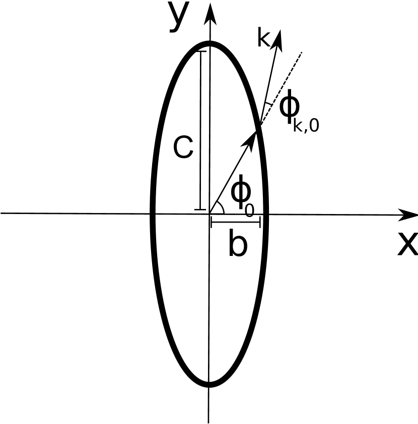
Figure 1.— The basic vortex geometry. A sample streamline is in bold, with semi-minor axis b and semi-major axis c. The ellipticity $\chi=c/b=4$ in this case. $\phi_{0}$ shows the initial angle of the radius vector with the $x$ axis while $\phi_{k,0}$ is the initial angle of the perturbation wavevector $\mathbf{k}$ with respect to the radius vector.

Taking the equilibrium solution (eq.[8] and [9]) posed above, we find

$$\mathfrak{L}=\omega\left(\begin{array}[]{cc}0&\chi^{-1}\\ -\chi&0\end{array}\right).$$ (40)

Using this result to solve equations (38) and (39), we find

$$x = b\cos(\omega t+\phi_{0}),$$ (41)

$$y = -\chi b\sin(\omega t+\phi_{0}),$$ (42)

$$k_{x} = k_{0}\cos(\omega t+\phi_{k,0}),$$ (43)

$$k_{y} = -\chi^{-1}k_{0}\sin(\omega t+\phi_{k,0}),$$ (44)

where $\phi_{0}$ and $\phi_{k,0}$ are the initial phase of the coordinate and the wavevector and $b$ is the semi-minor axis of the elliptical streamline (see figure 1). We can also use the result $\mbox{\boldmath{$k$}}\cdot\tilde{\mbox{\boldmath{$u$}}}=0$ (eq. [29]) to write

$$\tilde{u}_{x} = a(b,t)\sin(\omega t+\phi_{k,0}),$$ (45)

$$\tilde{u}_{y} = a(b,t)\chi\cos(\omega t+\phi_{k,0}),$$ (46)

where $a(b,t)$ determines the overall normalization of $\tilde{\mbox{\boldmath{$u$}}}$. Applying the results of equations (45) - (46) to equations (35) and (37), we find

$$\frac{d{a}}{dt} = 2\Lambda^{-1}\omega\left(\chi^{2}-1\right)\cos(\omega t+\phi_{k,0})\sin(\omega t+\phi_{k,0})a$$ (47)

$$+\Lambda^{-1}\left[\left(\omega^{2}+3\Omega^{2}\right)\cos(\omega t+\phi_{0})\sin(\omega t+\phi_{k,0})\right.$$

$$-\chi^{2}\omega^{2}\sin(\omega t+\phi_{0})\cos(\omega t+\phi_{k,0})$$

$$\left.-2\Omega\omega\chi\sin(\phi_{k,0}-\phi_{0})\right]b\frac{\tilde{\rho}}{\rho},$$

$$\frac{d{\tilde{\rho}}}{dt} = -a\sin(\phi_{k,0}-\phi_{0})\frac{\partial{\rho}}{\partial b},$$ (48)

where $\Lambda=\chi^{2}\cos^{2}(\omega t+\phi_{k,0})+\sin^{2}(\omega t+\phi_{k,0})$. Without loss of generality, we can choose $\phi_{0}=0$. Thus, equations (47) and (48) depend only on the initial angle of the wavevector, $\phi_{k,0}$. Equation (47) explicitly depends on the semi-minor axis $b$. However, because $b$ is independent of time and appears only in the $\tilde{\rho}$ term in combination with $\rho$, we can eliminate it by absorbing it into the background density gradient, replacing $\partial\rho/\partial b$ with $\partial\ln\rho/\partial\ln b$ in equation (48).

The first term on the RHS of equation (47) results from the first two terms of equation (35). The second term results from the density gradient within the vortex. For a zero density gradient, the integral over a period $T=2\pi\omega^{-1}$ of equation (47) is zero as this first term on the RHS is an odd function. Hence, in the absence of a density gradient, no exponentially growing modes exists in two dimensions. In addition, for an initially aligned wavevector (i.e. $\phi_{k,0}=0$) and $\tilde{\rho}(t=0)=0$, there is also no growth, regardless of the presence of a density gradient.

Equations (48) and (47) constitute a system of linear ODEs, which depends on initial conditions for $a$ and $\tilde{\rho}$, the initial angle of the wavevector $\phi_{k,0}$, the background density profile, $\partial\rho/\partial b$, and the vortex ellipticity, $\chi$. However, as we are interested in the asymptotic behavior of perturbations, i.e., growth or no growth, we are interested in the parameter range of $\phi_{k,0}$, $\chi$, and $\partial\rho/\partial b$, which yield stability or instability. To this end, we define a growth rate $\gamma$ where $\tilde{\rho}(t=\tau)=e^{\gamma\tau}f(\tau)$ and $f(t)$ is a period function over the vortex rotation period, $\tau=2\pi/\omega$. To find $\gamma$, we follow the general procedure of Floquet analysis on equations (47) and (48). For linearly independent initial conditions, e.g., $(a(t=0)=1,\tilde{\rho}(t=0)=0)$ and $(a(t=0)=0,\tilde{\rho}(t=0)=1)$, we can integrate equations (47) and (48) over one period $2\pi/\omega$ and solve for the most unstable eigenvalue of the resulting matrix (e.g. Bender & Orszag, 1978; Lesur & Papaloizou, 2009a).

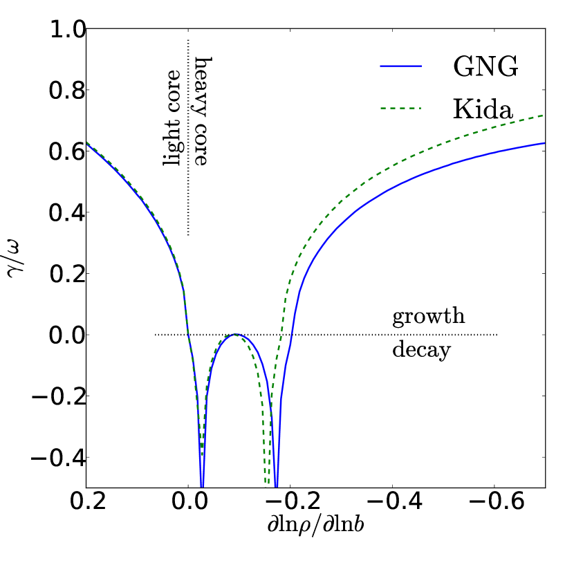
Figure 2.— Stability of protoplanetary vortices as a function of the density contrast. For any vortex that has a light core, i.e., $d\ln\rho/d\ln b>0$, we find a purely growing instability, i.e., the Vortical Rayleigh-Taylor Instability, which we discuss in §3.3. For sufficiently heavy cores, there is an instability, which we discuss in §3.4.

In Figure 2 we show the effect of different density contrasts on the growth rate for fixed $\chi=10$. Here we consider both light cores ($\partial\ln\rho/\partial\ln b>0$) and heavy cores ($\partial\ln\rho/\partial\ln b<0$). There are two regions of instability: one for light cores and and one for sufficiently heavy cores, which we discuss below. We show the effect of the vortex ellipticity $\chi$ on $\gamma$ in Figure 3 for the GNG (solid lines) and the Kida (dashed lines) for the light cores (light lines) and heavy cores (heavy lines).

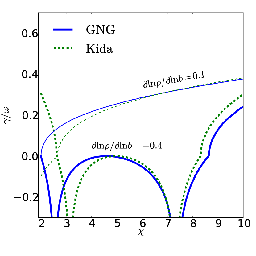
Figure 3.— Stability of protoplanetary vortices as a function of the $\chi$. For any vortex that has a light core, i.e., $d\ln\rho/d\ln b>0$, we find a purely growing instability for any value of $\chi>2$. For sufficiently heavy cores, i.e., the $\partial\ln\rho/\partial\ln b=-0.4$ case, Instability also demands a sufficiently large $\chi$.

For the light core case, we find that as $\chi$ increases, the growth rate in terms of $\omega$ also increases. However, there is generally always growth (with the exception of the low $\chi$ Kida case). In the heavy core case, there is no growth until $\chi$ is sufficiently large and the core sufficiently dense compared to the ambient flow. We summarized the growth rate for $\phi_{k,0}=\pi/2$ as a function of both $\chi$ and $\partial\ln\rho/\partial\ln b$ in Figure (4). In the case of the light core, $\partial\ln\rho/\partial\ln b>0$, we find instability for any density contrast. The heavy core case is more complicated. For small $\partial\ln\rho/\partial\ln b$ and small $\chi$, there is no instability. However, once $\partial\ln\rho/\partial\ln b$ and $\chi$ are sufficiently large, growth sets in. Growth can occur for smaller $\partial\ln\rho/\partial\ln b>0$ if $\chi$ is larger. In between the two regions of growth, i.e., light cores and sufficiently heavy cores, $\gamma<0$, indicating damping. The two heavy white lines marks the region of neutral stability. The physics of instability of these two light and heavy core cases are somewhat different, which we now discuss in §3.3 and §3.4.

Figure 4.— Growth rates as a function of $\chi$ and $\partial\ln\rho/\partial\ln b$ for the GNG vortex. The heavy white contour denotes the stability boundary ($\gamma/\omega=0$).

3.3. Vortices with Light Cores

The instability mechanism for light cores is analogous to the Rayleigh-Taylor instability. Recall that the protoplanetary vortices are high pressure regions. The pressure forces thus point outward and must be balance by a combination of centripetal and centrifugal forces which must point inward. If we ”unroll” this vortex, we see that the combination of centripetal and centrifugal forces, which oppose the pressure force, is analogous to gravity in a pressure support atmosphere. Hence, a light core in this context is equivalent to making the material less dense where the pressure is largest, i.e., putting denser material on top of less dense material. This is subject to a Rayleigh-Taylor-like instability, which we call the Vortical Rayleigh-Taylor Instability (VRTI). In the appendix, we present a simple example of this instability in a terrestial vortex to make more precise the analogy between the Rayleigh-Taylor Instability (RTI) and the VRTI. We note, however, that in the terrestial example presented in the appendix that the condition for instability is a heavy core as opposed to a light core. This results from the fact that terrestial vortices are low pressure regions, whereas protoplanetary vortices are high pressure regions.

We now demonstrate the behavior of perturbations for light cores by plugging $\omega$ for GNG (or Kida) vortices (eq. [18]) into equation (47), we integrate the evolution of equations (47) and (48) over several periods. We note that equation (47) admits a purely analytic solution when $\tilde{\rho}=0$. Integrating both sides with this in mind, we find

$$a(t)=a_{0}\frac{\chi^{2}+(1-\chi^{2})\sin^{2}\left(\phi_{k,0}\right)}{\chi^{2}+(1-\chi^{2})\sin^{2}\left(\omega t+\phi_{k,0}\right)},$$ (49)

where $a_{0}$ is fixed by initial conditions. The analytic solution (49) represents the evolution of a perturbation that is purely advected along in the flow. More complex cases are solved numerically.

Figure 5 shows the behavior of $a(t)$ and $\tilde{\rho}(t)$ for the initial conditions $a(t=0)=1$ and $\tilde{\rho}(t=0)=0$ and a background density profile of $\partial\ln\rho/\partial\ln b=0.01$, i.e., a light core. The background density profile corresponds to a one percent decrease in the density across the vortex. The velocity amplitude $a(t)$ for the $\phi_{k,0}=0$ case shows oscillatory behavior between 1 and 100, but no long term growth occurs. Correspondingly, the density perturbation remains zero for all time and is not shown in the right panel. Indeed, the solution’s behavior precisely follows the analytic result of equation (49), verifying the accuracy of our numerical integration. On the other hand, both $\phi_{k,0}=\pi/4$ and $\phi_{k,0}=\pi/2$ show significant growth, and the asymptotic growth rate, i.e., the slope of the trend, is maximized for $\pi/2$. This is unsurprising given the discussion in the appendix and the analogy with the RTI, where we found that growth rates are maximized when the wavevector is parallel to vortex streamlines.

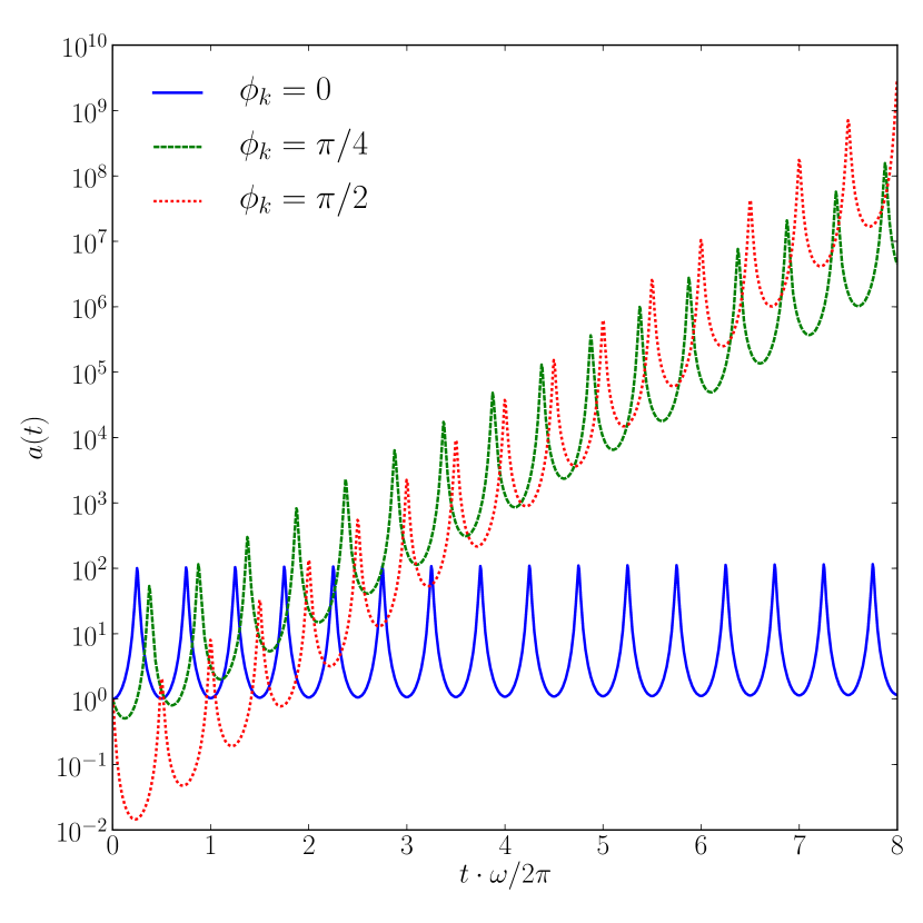
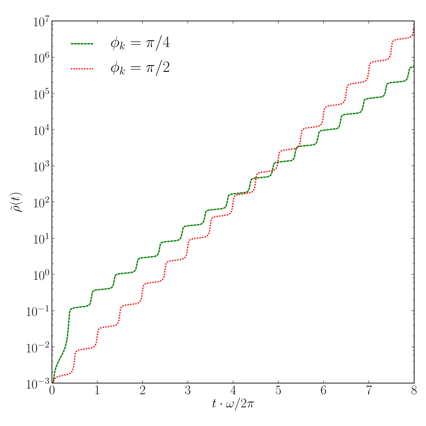
Figure 5.— Velocity (left) and density (right) perturbations as a function of time for three initial wavevector orientation angles $\phi_{k,0}$ for light cores ($\partial\ln\rho/\partial\ln b=0.01$). Note that $\phi_{k}=0$ has been dropped from the right plot because it has zero growth. This case is show on the left plot for illustrativ purposes. There is no growth for the $\phi_{k,0}=0$ case, and the growth rate is maximum for for $\phi_{k,0}=\pi/2$.

Similarly, we plug in $\omega$ for Kida vortices (eq. [22]) into equation (47) and integrate its evolution over several periods. Before comparing the behavior of the Kida vortices with that of the GNG vortices, we first note that from Figure 5, the velocity and density shows both short timescale periodic fluctuations, a result of the spatially inhomogeneous flow field, i.e., vortex, and long term behavior. As we are only interested in long term behavior, we sample $\tilde{\rho}$ where $\omega t$ is an integer multiple of $2\pi$ for both vortices and show the results in Figure 6. The comparison clearly shows that the background state makes no difference in the qualitative behavior of the instability and little difference in the quantitative behavior of the growth rate.

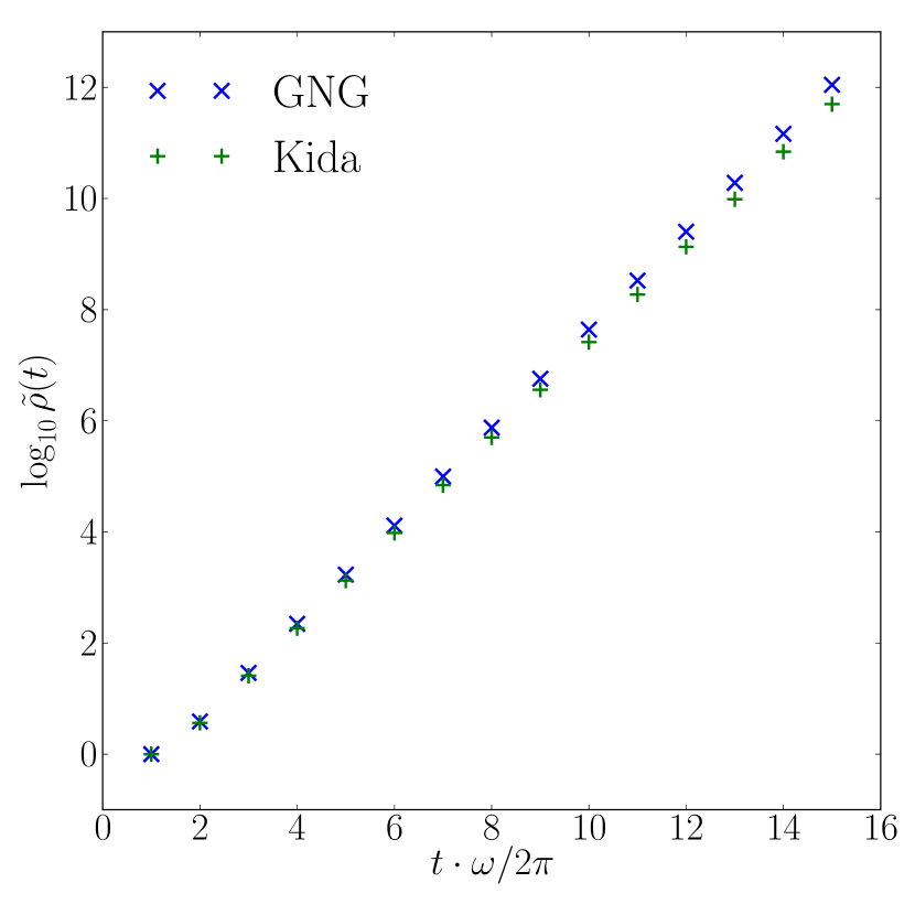
Figure 6.— A comparison of the GNG and Kida background states for the $\phi_{k,0}=\pi/2$, $\chi=5$ case for the light core case ($\partial\ln\rho/\partial\ln b=0.01$). The figure shows density perturbation as a function of time for both background states.

3.4. Vortices with Heavy Cores

We now discuss the heavy core case. To help elucidate the physics, we first consider the effective gravity that counteract the pressure forces in a GNG vortex, i.e., $\rho^{-1}\partial P/\partial x=-g_{x},\ \rho^{-1}\partial P/\partial y=-g_{y}$. From equation (19), we know that the pressure drop between vortex streamlines is constant. Hence, the effective gravity is

$$g_{x} = -\rho^{-1}\frac{\partial P}{\partial b}\frac{db}{dx}$$ (50)

$$g_{y} = -\rho^{-1}\frac{\partial P}{\partial b}\frac{db}{dy},$$ (51)

where $b=\sqrt{x^{2}+y^{2}/\chi^{2}}$. Hence computing the magnitude of the effective gravity is, thus,

$$g=\sqrt{g_{x}^{2}+g_{y}^{2}}=g_{0}\sqrt{\cos^{2}\phi+\frac{\sin^{2}\phi}{\chi^{2}}},$$ (52)

where

$$g_{0}=b\Omega^{2}\left(\frac{3\chi^{2}}{\chi^{2}-1}-2\sqrt{\frac{3\chi^{2}}{\chi^{2}-1}}\right)={\rm const}.$$ (53)

We now plot the behavior of the effective gravity ($\hat{g}(t)=g(t)/g_{0}$) and the growing perturbations ($a(t)$ and $\tilde{\rho}(t)$) in Figure 7 for $\phi_{k,0}=\pi/2$. Note that perturbed density ($\tilde{\rho}(t)$) and velocity ($a(t)$) changes only at intervals where $g(t)$ is large. This is unsurprising for large $\chi$, the effective gravity will vary between $g_{0}/\chi$ and $g_{0}$. These peaks in the effective gravity is reached for $y=0$, i.e., on the minor axis of the elliptical vortex. This is reasonable from a physical perspective as it is here that the distance between vortex streamlines is minimal while the pressure change between vortex streamlines remain unchanged (for GNG vortices). Thus, the force is maximal there.

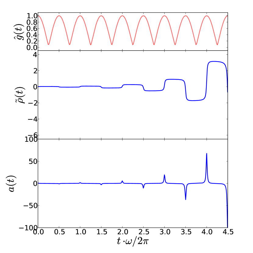
Figure 7.— The effective gravitational acceleration $\hat{g}(t)=g(t)/g_{0}$ normalized to the maximum gravitational acceleration, perturbed density (in arbitrary units), and $a(t)$ (again in arbitary units). Note that the peaks of $g(t)$ correspond to the peaks in $a(t)$ and changes in $\tilde{\rho}(t)$, which correspond to periodic kicks at roughly half the rotation period of the vortex.

This effective gravity, which is time dependent (as fluid is advected along a vortex), is akin to a kick. The relative strength of these kicks depend on $\chi$ and the period of these kicks is exactly half of the rotation period of the vortex as a fluid element moving along a streamline crosses the minor axis twice a rotation period. As the modes we are following is akin to radial gravity modes, the density contrast determines their period. Hence, the minimum density contrast required for instability has an obvious intepretation: the radial gravity mode must also have a period that is comparable to the rotation period of the vortex to it to couple successfully to the kick and develop overstable oscillations as the plot of $\tilde{\rho}$ in Figure 7 shows. In addition, the minimum $\chi$ needed for instability as demonstrated in Figure 3 and 4 results from requiring each kick to be sufficiently strong.

Similarly, we can make the same comparison between the GNG and Kida vortex in the heavy core case in Figure 8 as we have done in the light core case in Figure 6. Again, we plug in $\omega$ for Kida vortices (eq. [22]) into equation (47) and integrate its evolution over several periods but this time for a background density gradient of $\partial\ln\rho/\partial\ln b=-0.3$ and $\chi=12$. Again we discard short timescale periodic fluctuations and sample $\tilde{\rho}$ where $\omega t$ is an integer multiple of $2\pi$ for both vortices. The comparison shows that the growth rate of the HCI is more dependent on the vortex solution (Kida vs. GNG) than the VRTI. Whereas Figure 6 shows that the amplitude of the density perturbation for the Kida and GNG vortices track each other fairly closely, these amplitude diverge much more strongly in the HCI as shown in Figure 8.

Figure 8.— Same as Figure 6 except for the heavy core case. Here $\chi=12$ and $\partial\ln\rho/\partial\ln b=-0.3$.

4. Discussion

The analysis of the preceding section demonstrates that vortices with light cores or sufficiently heavy cores are unstable to the VRTI and HCI respectively. Figures 2 and 4 shows that growth occurs on a few vortex rotation periods. Moreover, these instability appears to be robust and its detailed physics are independent of the vortex model used (either GNG or Kida). Having demonstrated the basic physics of these instabilities, we turn now to its application to planetesimal formation. We will first review some of the physics of dust trapping in vortices.

If planetesimals form by gravitational collapse and fragmentation of a dust sublayer (Safronov, 1972; Goldreich & Ward, 1973), then this layer must have a Toomre, $Q<1$ (but also see Ward 2000), which implies that the velocity dispersion of the sublayer must be below:

$$\sigma_{\rm d}<\frac{\pi G\Sigma_{\rm d}}{2\Omega}\approx 5\,{\rm cm\,s}^{-1}$$ (54)

for the minimal mass solar nebula (MMSN), where $\Sigma_{\rm d}$ is the surface density of the dust layer. For a laminar disk, this criterion is amply fulfilled if the dust is allowed to settle to the midplane. However, as the dust collects near the midplane, it is subject the induced Kelvin-Helmholtz instabilities with the overlying gas layers (Weidenschilling & Cuzzi, 1993; Cuzzi et al., 1993; Chiang, 2008; Barranco, 2009). Therefore, the dispersion of the dust layer is closer to a few ${\rm m\,s}^{-1}$. Hence the surface density must be enhanced by a factor of $\sim 20-100$ (effectively the $Q$ of the gaseous disk) so that gravitational instability can operate (Chavanis, 2000).

More careful considerations suggest this enhancement of $\sim 20-100$ may be a severe overestimate and that only enhancement of order a few is needed in the high metallicity disks which preferentially form planets (Youdin & Shu, 2002; Johansen et al., 2009). In any case, vortices are one avenue by such a dust surface density enhancement can be achieved as Barge & Sommeria (1995) first pointed out. The timescale for dust to connect and concentrate in vortices, i.,e., the capture timescale, $t_{\rm capt}$, can be fairly rapid, i.e., $t_{\rm capt}\sim t_{\rm dyn}$, when $t_{\rm stop}\sim t_{\rm dyn}$ as pointed out by Barge & Sommeria (1995); Tanga et al. (1996); Chavanis (2000). Over the lifetime of a vortex, $t_{\rm life}$, the amount of dust the can be gathered by a vortex is very large. Chavanis (2000) argues that this mass is

$$M_{\rm d}\sim\Omega t_{\rm life}\Sigma_{\rm d}R^{2}f^{2}(t_{\rm stop}),$$ (55)

where $f$ describes the efficiency of capturing dust and is $\sim 1$ when $t_{\rm stop}\sim t_{\rm dyn}$ and $R$ is the size scale of the vortex. If the inward concentration of dust is balanced by the outward diffusion of this dust concentration due to turbulence, these dust particles would be confined to a region on a scale of

$$r_{\rm d}\sim\sqrt{Dt_{\rm capt}},$$ (56)

where $D\sim\alpha R^{2}\Omega$ is the turbulent diffusivity. For $\alpha=0.01$, $r_{\rm d}\sim 0.1R$, i.e., in the central core of the vortex. Hence the surface density is enhanced by two orders of magnitude. Since the GI hypothesis for planetesimal formation only demands more modest increases, vortices should be ideal sites of planetesimal formation.

However, such a increase in dust surface density is not without its costs. As we have shown a sufficient increase in the effective mean molecular weight of the gas in the cores of vortices is destabilizing. The condition for the HCI demands a mean molecular weight increase of order 20% or an increase of the dust surface density by a factor of 20% if the dust and gas densities are similar in the midplane. This increase in dust surface density is much smaller than what is required for the GI hypothesis, which demands a factor of a few increase (Youdin & Shu, 2002; Chiang & Youdin, 2009) if the vertical structure of dust is taken into account to a factor of $20-100$ when vertical structure is ignored (Chavanis, 2000). Thus, the HCI will be triggered before gravitational instability sets in according to the present linear calculation.

There are many issues involving the stability of vortices with a heavy core than cannot be resolved by the present linear calculation, which we now briefly discuss. The first issue is the non-linear state of the instability, which is not known at present. We expect the HCI to grow until its saturates, which may 1. destroy the vortex, 2. increase the velocity dispersion of the dust layer, or 3. limit the enhancement in the dust surface density to a few tens of percent, i.e., marginal stability. For any of these options, GI is curtailed in cores of vortices.

Another issue is the equilibrium distribution of dust along a streamline. We have assumed that the dust is uniformly distributed along a streamline. For light particles, this is likely the case. Tanga et al. (1996) and Chavanis (2000) studied the process of dust trapping in vortices and found that the zeroth order motion is that light particles of dust travels along the elliptical streamlines with a slow ”radial” drift due to drag forces. However, heavy particles move along epicycles, i.e., ellipses with aspects ratio 2. In addition, Youdin (2008) showed that the stationary point for dust in a sub-Keplerian gas is not the center of the vortex, but rather a point that is forward in azimuth. This is unsurprising as the dust, in maintaining a sub-Keplerian rotation rate, demands an additional radial force away from the central star to counteract gravity, a force that is supplied by gas pushing on the dust if the dust is ahead of the vortex center in azimuth. These elements suggest that the distribution of dust along a streamline may not be uniform and so may affect the stability properties of vortices in a non-trivial way.

A third issue is the nature of gas-dust coupling. We have assumed the gas and dust are well coupled on a dynamical time. However, this may not be the case. For instance, the fastest settling dust is that which is marginally coupled to the gas, i.e., $\Omega t_{\rm s}=1$, where $t_{\rm s}$ is the dust stopping time, (Johansen et al., 2004). The dust that is trapped in vortices may be preferentially of a certain size, i.e., marginally coupled to the gas. Hence the instability growth time, dynamical time, and dust-gas coupling time, in the dusty protoplanetary disk can be all of the same order.

Additional instabilities that arise directly from this gas-dust coupling may also be important. Youdin & Goodman (2005) showed that the imperfect coupling between gas and dust and their backreaction on each other leads to a secular streaming instability. This instability leads to protoplanetary disk turbulence and tends to concentrate dust Youdin & Johansen (2007); Johansen & Youdin (2007). These streaming instabilities or analogues may also be important in the stability protoplanetary vortices and would be profitable to explore. A proper accounting of gas-dust coupling in a vortex and its effect on the VRTI is a topic of future work.

Another issue is that the vertical structure of the gas and the dust is very different in protoplanetary disks. Dust tends to settle toward the midplane (though the presence of vortices and/or turbulence may counter this tendency). This settled dust may drive vertical turbulence if it is sufficiently concentrated (see for instance Chiang, 2008; Barranco, 2009). The effect of this difference in the vertical structure of gas and dust on vortices has not yet been addressed and is likely important for both their equilibrium and stability. However, we may expect the HCI to be important regardless because is a 2-D effect in a thin dust layer within a thicker gas vortex.

Finally, the alert reader (and referee) will note that we have not discussed the case of $1<\chi<2$ vortices, i.e., low pressure vortices. In principle, such vortices might exist in protoplanetary discs, but the prevailing theoretical bias is that vortices in protoplanetary discs are high pressure regions. We have gone along with this bias in this work and have ignored these low pressure vortices. However, we note that heavy core low pressure vortices are violently unstable (equivalent to the light core case discussed above) because of the reversal in the direction of the effective gravity. In addition, it is unclear if these vortices would concentrate dust. The equivalent calculation of Chavanis (2000) for low pressure vortices has not been performed. While a detailed study of low pressure protoplanetary vortices might be interesting, the impact of such a study is unclear.

5. Conclusions and Open Issues

We have demonstrated two instabilities in protoplanetary vortices, resulting from light cores (VRTI) and sufficiently heavy cores (HCI). The physics of the VRTI is analogous to the Rayleigh-Taylor instability, with gravity replaced by centrifugal and centripetal forces in a rotating fluid. The HCI appears to be a parametric instability. We have shown that these instabilities are robust for all vortices possessing a light or sufficiently heavy core. For protoplanetary vortices, the instability of interest is the HCI as dust would concentrate in their centers, leading to heavy cores. While the nonlinear state of the these remains unexplored, we expect that this instability prevents vortices from acting as protoplanetary nurseries.

Both the VRTI and HCI are novel among elliptical vortex instabilities as they are 2-D – only motions in the x-y plane are required. Previous work on the stability of vortices have focused on the importance of the instabilities that involve 3-D motions (Lithwick, 2009; Lesur & Papaloizou, 2009a). Indeed, 3-D effects do lead to additional instabilities that destroy vortices even before they can collect dust. Lesur & Papaloizou (2009a) argued that the 3-D elliptical instability can destroy Kida vortices for $\chi<4$ and $\chi>6$. Lithwick (2009) argues that nonlinear coupling and transient amplification between a vortex and its children that involve a vertical component leads to destruction of the vortex. He argues that the stability requirement for any vortex is then that the base of the vortex be larger (by at least a factor of 2) than its height. Our results suggest that if gas vortices having $\chi\gtrsim 6$ (as proposed by Lithwick (2009)), the HCI will affect these vortices as they gather dust.

The analysis that we have attempted here is linear and so it is highly dependent on the background equilibrium state. The two equilibria (Kida and GNG) that we have analyzed in this paper were chosen due to their simple analytic structure. Although we have shown that the HCI is very similar in both these cases, 3-D simulations have clearly demonstrated that vortices in protoplanetary disks are not so simple Barranco & Marcus (2005); Shen et al. (2006); Lithwick (2009).

Finally, our work leaves open a number of issues including the nonlinear state of the HCI, gas-dust coupling physics, and equilibrium structure and vertical structure of vortices. We are currently pursuing numerical work exploring the effects of heavy vortices in protoplanetary disk.

Appendix A A Simple Example of Vortical Rayleigh-Taylor Instability

In this appendix, we discuss a simple example of the Vortical Rayleigh-Taylor instability (VRTI) in a terrestrial vortex to illustrate its basic physics. Our simple treatment is derived from Sipp et al. (2005), and a detailed overview of the state of terrestrial heavy vortex instability theory is found therein.

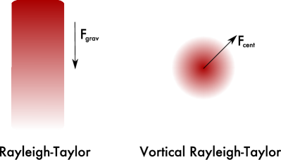
Figure 9.— A cartoon showing the salient feature of the Rayleigh-Taylor type instability, which is that the density gradient (represented by the shading: dark tones correspond to high density, light tones to low density) is in the opposite direction from the restoring force. In the case of the standard Rayleigh-Taylor instability, the force is gravity; in the vortical Rayleigh-Taylor case it is the centrifugal force.

For a 2-d circular vortex in equilibrium, pressure forces (inward) are counterbalanced by centrifugal forces (outward). Incompressible motions of this 2-d vortex are described by the continuity equation,

$$\frac{\partial{\rho}}{\partial t}+u\frac{\partial{\rho}}{\partial r}+\frac{v}{r}\frac{\partial{\rho}}{\partial\phi}=0,$$ (A1)

where $\rho$ is the density, $u=\dot{r}$ and $v=r\dot{\phi}$, the momentum equations,

$$\frac{\partial{u}}{\partial t}+u\frac{\partial{u}}{\partial r}+\frac{v}{r}\frac{\partial{u}}{\partial\phi}-\frac{v^{2}}{r} = -\frac{1}{\rho}\frac{\partial{P}}{\partial r},$$ (A2)

$$\frac{\partial{v}}{\partial t}+u\frac{\partial{v}}{\partial r}+\frac{v}{r}\frac{\partial{v}}{\partial\phi}+\frac{uv}{r} = -\frac{1}{\rho r}\frac{\partial{P}}{\partial\phi},$$ (A3)

where $P$ is the pressure, and the incompressibility condition,

$$r^{-1}\frac{\partial{ru}}{\partial r}+\frac{1}{r}\frac{\partial{v}}{\partial\phi}=0.$$ (A4)

In equilibrium, the fluid motions of the vortex are circular and constant, i.e., $u=0$ and $v$ is constant. Hence we find that

$$\rho^{-1}\frac{\partial{P}}{\partial r}=\frac{v^{2}}{r}.$$ (A5)

We now perturb equations (A1)-(A4) and assume perturbations of the form $\exp(-i\omega t+im\phi+ikr)$. The perturbed continuity and momentum equations read

$$-i\bar{\sigma}\delta\rho+\delta u\frac{\partial{\rho}}{\partial r} = 0$$ (A6)

$$-i\bar{\sigma}\delta u-\frac{2v}{r}\delta v = -ik\frac{\delta P}{\rho}+\frac{1}{\rho}\frac{\partial{P}}{\partial r}\frac{\delta\rho}{\rho}$$ (A7)

$$-i\bar{\sigma}\delta v+\left(\frac{\partial{v}}{\partial r}+\frac{v}{r}\right)\delta u = -i\frac{m}{r}\frac{\delta P}{\rho},$$ (A8)

where $\bar{\sigma}=\left(\omega-{mv}/r\right)$. The incompressibility condition (eq.[A4]) becomes

$$ik\delta u+\frac{im}{r}\delta v=0,$$ (A9)

where we have assumed $kr\gg 1$. Equation (A9) gives $\delta v$ in terms of $\delta u$, which we apply to equations (A7) and (A8). Using equation (A6) for $\delta\rho$ in terms of $\delta u$, we find the dispersion relation:

$$\bar{\sigma}^{2}\left(\frac{m^{2}}{r^{2}}+k^{2}\right)+i\bar{\sigma}k\frac{m}{r}\left(\frac{\partial{v}}{\partial r}-\frac{v}{r}\right)-\frac{m^{2}}{r^{2}}\frac{v^{2}}{r}\frac{\partial{\ln\rho}}{\partial r}=0.$$ (A10)

For an uniformly rotating vortex, $v\propto r$, the second term in (A10) vanishes and the solution to the dispersion relation is

$$\bar{\sigma}^{2}=\frac{m^{2}/r^{2}}{m^{2}/r^{2}+k^{2}}\frac{v^{2}}{r}\frac{\partial{\ln\rho}}{\partial r},$$ (A11)

which is $<0$ (unstable) if $\partial{\ln\rho}/\partial r<0$, that is, if the core of the vortex is heavy. This instability is analogous to the Rayleigh-Taylor instability, whose dispersion relation is $\omega\propto k_{\perp}^{2}/k^{2}$, but where gravity is replaced by a centrifugal force. In the case of the Rayleigh-Taylor instability, the equilibrium is set by pressure forces balancing gravity. Heavy fluid that sits on top of light fluid which fulfills the conditions of equilibrium, but is unstable to interpenetration across the interface. By analogy, in the VRTI case, the equilibrium vortex is set by pressure forces balancing centrifugal forces. The presence of a heavy core leads to non-axisymmetric instabilities (where the origin is set by the center of the vortex), where again the heavy fluid elements in the core interpenetrate light fluid on the exterior. Figure 9 illustrates this analogy.

The analogy is made clearer if we identify $k_{\phi}\equiv m/r$, which is perpendicular to the centrifugal force (i.e., the effective gravity), which is in the $\hat{r}$ direction. Thus, we can make the identification $k_{\phi}^{2}/({k_{\phi}^{2}+k^{2}})\leftrightarrow k_{\perp}^{2}/k^{2}$ between VRTI and RTI, respectively. The wavevector that grows the fastest in both instabilities is the wavevector that is perpendicular to the vertical gravity and the radially outward centrifugal force, respectively.

References

- Barge & Sommeria (1995) Barge, P., & Sommeria, J. 1995, A&A, 295, L1
- Barranco (2009) Barranco, J. A. 2009, ApJ, 691, 907
- Barranco & Marcus (2005) Barranco, J. A., & Marcus, P. S. 2005, ApJ, 623, 1157
- Bayly (1988) Bayly, B. J. 1988, Physics of Fluids, 31, 56
- Bender & Orszag (1978) Bender, C. M., & Orszag, S. A. 1978, Advanced Mathematical Methods for Scientists and Engineers, ed. S. A. Bender, C. M. & Orszag
- Bracco et al. (1999) Bracco, A., Chavanis, P. H., Provenzale, A., & Spiegel, E. A. 1999, Physics of Fluids, 11, 2280
- Chavanis (2000) Chavanis, P. H. 2000, A&A, 356, 1089
- Chiang (2008) Chiang, E. 2008, ApJ, 675, 1549
- Chiang & Youdin (2009) Chiang, E., & Youdin, A. 2009, to appear in ARAA, ArXiv e-prints
- Cuzzi et al. (1993) Cuzzi, J. N., Dobrovolskis, A. R., & Champney, J. M. 1993, Icarus, 106, 102
- Godon & Livio (2000) Godon, P., & Livio, M. 2000, ApJ, 537, 396
- Goldreich & Lynden-Bell (1965) Goldreich, P., & Lynden-Bell, D. 1965, MNRAS, 130, 125
- Goldreich & Ward (1973) Goldreich, P., & Ward, W. R. 1973, ApJ, 183, 1051
- Goodman et al. (1987) Goodman, J., Narayan, R., & Goldreich, P. 1987, MNRAS, 225, 695
- Johansen et al. (2004) Johansen, A., Andersen, A. C., & Brandenburg, A. 2004, A&A, 417, 361
- Johansen & Youdin (2007) Johansen, A., & Youdin, A. 2007, ApJ, 662, 627
- Johansen et al. (2009) Johansen, A., Youdin, A., & Mac Low, M. 2009, ApJ, 704, L75
- Kida (1981) Kida, S. 1981, Journal of the Physical Society of Japan, 50, 3517
- Lesur & Papaloizou (2009a) Lesur, G., & Papaloizou, J. C. B. 2009a, A&A, 498, 1
- Lesur & Papaloizou (2009b) —. 2009b, ArXiv e-prints
- Lifschitz & Hameiri (1991) Lifschitz, A., & Hameiri, E. 1991, Physics of Fluids, 3, 2644
- Lithwick (2009) Lithwick, Y. 2009, ApJ, 693, 85
- Lovelace et al. (1999) Lovelace, R. V. E., Li, H., Colgate, S. A., & Nelson, A. F. 1999, ApJ, 513, 805
- Lyra et al. (2009) Lyra, W., Johansen, A., Zsom, A., Klahr, H., & Piskunov, N. 2009, A&A, 497, 869
- Safronov (1972) Safronov, V. S. 1972, Evolution of the protoplanetary cloud and formation of the earth and planets., ed. V. S. Safronov
- Shen et al. (2006) Shen, Y., Stone, J. M., & Gardiner, T. A. 2006, ApJ, 653, 513
- Sipp et al. (2005) Sipp, D., Fabre, D., Michelin, S., & Jacquin, L. 2005, Journal of Fluid Mechanics, 526, 67
- Sipp & Jacquin (2000) Sipp, D., & Jacquin, L. 2000, Physics of Fluids, 12, 1740
- Tanga et al. (1996) Tanga, P., Babiano, A., Dubrulle, B., & Provenzale, A. 1996, Icarus, 121, 158
- Varnière & Tagger (2006) Varnière, P., & Tagger, M. 2006, A&A, 446, L13
- Ward (2000) Ward, W. R. 2000, in Origin of the earth and moon, edited by R.M. Canup and K. Righter and 69 collaborating authors. Tucson: University of Arizona Press., p.75-84, ed. Canup, R. M., Righter, K., & et al., 75–84
- Weidenschilling & Cuzzi (1993) Weidenschilling, S. J., & Cuzzi, J. N. 1993, in Protostars and Planets III, ed. E. H. Levy & J. I. Lunine, 1031–1060
- Youdin (2008) Youdin, A. 2008, ArXiv e-prints
- Youdin & Johansen (2007) Youdin, A., & Johansen, A. 2007, ApJ, 662, 613
- Youdin & Goodman (2005) Youdin, A. N., & Goodman, J. 2005, ApJ, 620, 459
- Youdin & Shu (2002) Youdin, A. N., & Shu, F. H. 2002, ApJ, 580, 494