Performance Bounds for Expander-Based Compressed Sensing in Poisson Noise

Abstract

This paper provides performance bounds for compressed sensing in the presence of Poisson noise using expander graphs. The Poisson noise model is appropriate for a variety of applications, including low-light imaging and digital streaming, where the signal-independent and/or bounded noise models used in the compressed sensing literature are no longer applicable. In this paper, we develop a novel sensing paradigm based on expander graphs and propose a MAP algorithm for recovering sparse or compressible signals from Poisson observations. The geometry of the expander graphs and the positivity of the corresponding sensing matrices play a crucial role in establishing the bounds on the signal reconstruction error of the proposed algorithm. We support our results with experimental demonstrations of reconstructing average packet arrival rates and instantaneous packet counts at a router in a communication network, where the arrivals of packets in each flow follow a Poisson process.

I Introduction

The goal of compressive sampling or compressed sensing (CS) [1, 2] is to replace conventional sampling by a more efficient data acquisition framework, which generally requires fewer sensing resources. This paradigm is particularly enticing whenever the measurement process is costly or constrained in some sense. For example, in the context of photon-limited applications (such as low-light imaging), the photomultiplier tubes used within sensor arrays are physically large and expensive. Similarly, when measuring network traffic flows, the high-speed memory used in packet counters is cost-prohibitive. These problems appear ripe for the application of CS.

However, photon-limited measurements [3] and arrivals/departures of packets at a router [4] are commonly modeled with a Poisson probability distribution, posing significant theoretical and practical challenges in the context of CS. One of the key challenges is the fact that the measurement error variance scales with the true intensity of each measurement, so that we cannot assume constant noise variance across the collection of measurements. Furthermore, the measurements, the underlying true intensities, and the system models are all subject to certain physical constraints, which play a significant role in performance.

Recent works [5, 6, 7, 8] explore methods for CS reconstruction in the presence of impulsive, sparse or exponential-family noise, but do not account for the physical constraints associated with a typical Poisson setup and do not contain the related performance bounds emphasized in this paper. In previous work [9, 10], we showed that a Poisson noise model combined with conventional dense CS sensing matrices (properly scaled) yielded performance bounds that were somewhat sobering relative to bounds typically found in the literature. In particular, we found that if the number of photons (or packets) available to sense were held constant, and if the number of measurements, $m$, was above some critical threshold, then larger $m$ in general led to larger bounds on the error between the true and the estimated signals. This can intuitively be understood as resulting from the fact that dense CS measurements in the Poisson case cannot be zero-mean, and the DC offset used to ensure physical feasibility adversely impacts the noise variance.

The approach considered in this paper hinges, like most CS methods, on reconstructing a signal from compressive measurements by optimizing a sparsity-regularized goodness-of-fit objective function. In contrast to many CS approaches, however, we measure the fit of an estimate to the data using the Poisson log-likelihood instead of a squared error term. This paper demonstrates that the bounds developed in previous work can be improved for some sparsity models by considering alternatives to dense sensing matrices with random entries. In particular, we show that deterministic sensing matrices given by scaled adjacency matrices of expander graphs have important theoretical characteristics (especially an $\ell_{1}$ version of the restricted isometry property [11]) that are ideally suited to controlling the performance of Poisson CS.

Formally, suppose we have a signal $\theta^{*}\in\mathbb{R}_{+}^{n}$ with known $\ell_{1}$ norm $\|\theta^{*}\|_{1}$ (or a known upper bound on $\|\theta^{*}\|_{1}$). We aim to find a matrix ${\Phi}\in\mathbb{R}_{+}^{m\times n}$ with $m$, the number of measurements, as small as possible, so that $\theta^{*}$ can be recovered efficiently from the measured vector ${y}\in\mathbb{R}_{+}^{m}$, which is related to ${\Phi}\theta^{*}$ through a Poisson observation model. The restriction that elements of ${\Phi}$ be nonnegative reflects the physical limitations of many sensing systems of interest (e.g., packet routers and counters or linear optical systems). The original approach employed dense random matrices [11, 12]. It has been shown that if the matrix ${\Phi}$ acts nearly isometrically on the set of all $k$-sparse signals, thus obeying what is now referred to as the Restricted Isometry Property with respect to $\ell_{2}$ norm (RIP-2) [11], then the recovery of $\theta^{*}$ from ${\Phi}\theta^{*}$ is indeed possible. It has been also shown that dense random matrices constructed from Gaussian, Bernoulli, or partial Fourier ensembles satisfy the required RIP-2 property with high probability [11].

Adjacency matrices of expander graphs [13] have been recently proposed as an alternative to dense random matrices within the compressed sensing framework, leading to computationally efficient recovery algorithms [14, 15, 16]. It has been shown that variations of the standard recovery approaches such as basis pursuit [2] and matching pursuit [17] are consistent with the expander sensing approach and can recover the original sparse signal successfully [18, 19]. In the presence of Gaussian or sparse noise, random dense sensing and expander sensing are known to provide similar performance in terms of the number of measurements and recovery computation time. Berinde et al. proved that expander graphs with sufficiently large expansion are near-isometries on the set of all $k$-sparse signals in the $\ell_{1}$ norm; this is referred as a Restricted Isometry Property for $\ell_{1}$ norm (RIP-1) [18]. Furthermore, expander sensing requires less storage whenever the signal is sparse in the canonical basis, while random dense sensing provides slightly tighter recovery bounds [16].

The approach described in this paper consists of the following key elements:

• expander sensing matrices and the RIP-1 associated with them;

• a reconstruction objective function which explicitly incorporates the Poisson likelihood;

• a countable collection of candidate estimators; and

• a penalty function defined over the collection of candidates, which satisfies the Kraft inequality and which can be used to promote sparse reconstructions.

In general, the penalty function is selected to be small for signals of interest, which leads to theoretical guarantees that errors are small with high probability for such signals. In this paper, exploiting the RIP-1 property and the non-negativity of the expander-based sensing matrices, we show that, in contrast to random dense sensing, expander sensing empowered with a maximum a posteriori (MAP) algorithm can approximately recover the original signal in the presence of Poisson noise, and we prove bounds which quantify the MAP performance. As a result, in the presence of Poisson noise, expander graphs not only provide general storage advantages, but they also allow for efficient MAP recovery methods with performance guarantees comparable to the best $k$-term approximation of the original signal. Finally, the bounds are tighter than those for specific dense matrices proposed by Willett and Raginsky [9, 10] whenever the signal is sparse in the canonical domain, in that a log term in the bounds in [10] is absent from the bounds presented in this paper.

I-A Relationship with dense sensing matrices for Poisson CS

In recent work, the authors established performance bounds for CS in the presence of Poisson noise using dense sensing matrices based on appropriately shifted and scaled Rademacher ensembles [9, 10]. Several features distinguish that work from the present paper:

• The dense sensing matrices used in [9, 10] require more memory to store and more computational resources to apply to a signal in a reconstruction algorithm. The expander-based approach described in this paper, in contrast, is more efficient.

• The expander-based approach described in this paper works only when the signal of interest is sparse in the canonical basis. In contrast, the dense sensing matrices used in [9, 10] can be applied to arbitrary sparsity bases (though the proof technique there needs to be altered slightly to accommodate sparsity in the canonical basis).

• The bounds in both this paper and [9, 10] reflect a sobering tradeoff between performance and the number of measurements collected. In particular, more measurements (after some critical minimum number) can actually degrade performance as a limited number of events (e.g., photons) are distributed among a growing number of detectors, impairing the SNR of the measurements.

I-B Notation

Nonnegative reals (respectively, integers) will be denoted by $\mathbb{R}_{+}$ (respectively, $\mathbb{Z}_{+}$). Given a vector ${u}\in\mathbb{R}^{n}$ and a set $S\subseteq\{1,\ldots,n\}$, we will denote by ${u}^{S}$ the vector obtained by setting to zero all coordinates of ${u}$ that are in $S^{c}$, the complement of $S$: $\forall 1\leq i\leq n,u^{S}_{i}=u_{i}1_{\{i\in S\}}$. Given some $1\leq k\leq n$, let $S$ be the set of positions of the $k$ largest (in magnitude) coordinates of ${u}$. Then ${u}^{(k)}\stackrel{{\scriptstyle\scriptscriptstyle\triangle}}{{=}}{u}^{S}$ will denote the best $k$-term approximation of ${u}$ (in the canonical basis of $\mathbb{R}^{n}$), and

$$\sigma_{k}({u})\stackrel{{\scriptstyle\scriptscriptstyle\triangle}}{{=}}\|{u}-{u}^{(k)}\|_{1}=\sum_{i\in S^{c}}|u_{i}|$$

will denote the resulting $\ell_{1}$ approximation error. The $\ell_{0}$ quasinorm measures the number of nonzero coordinates of ${u}$: $\|{u}\|_{0}\stackrel{{\scriptstyle\scriptscriptstyle\triangle}}{{=}}\sum^{n}_{i=1}1_{\{u_{i}\neq 0\}}$. For a subset $S\subseteq\{1,\ldots,n\}$ we will denote by $I_{S}$ the vector with components $1_{\{i\in S\}}$, $1\leq i\leq n$. Given a vector ${u}$, we will denote by ${u}^{+}$ the vector obtained by setting to zero all negative components of ${u}$: for all $1\leq i\leq n$, $u^{+}_{i}=\max\{0,u_{i}\}$. Given two vectors $u,v\in\mathbb{R}^{n}$, we will write $u\succeq v$ if $u_{i}\geq v_{i}$ for all $1\leq i\leq n$. If $u\succeq\alpha I_{\{1,\ldots,n\}}$ for some $\alpha\in\mathbb{R}$, we will simply write $u\succeq\alpha$. We will write $\succ$ instead of $\succeq$ if the inequalities are strict for all $i$.

I-C Organization of the paper

This paper is organized as follows. In Section II, we summarize the existing literature on expander graphs applied to compressed sensing and the RIP-1 property. Section III describes how the problem of compressed sensing with Poisson noise can be formulated in a way that explicitly accounts for nonnegativity constraints and flux preservation (i.e., we cannot detect more events than have occurred); this section also contains our main theoretical result bounding the error of a sparsity penalized likelihood reconstruction of a signal from compressive Poisson measurements. These results are illustrated and further analyzed in Section IV, in which we focus on the specific application of efficiently estimating packet arrival rates. Several technical discussions and proofs have been relegated to the appendices.

II Background on expander graphs

We start by defining an unbalanced bipartite vertex-expander graph.

Definition II.1.

We say that a bipartite simple graph $G=(A,B,E)$ with (regular) left degree $d$ is a $(k,\epsilon)$-expander if, for any $S\subset A$ with $|S|\leq k$, the set of neighbors ${\cal N}(S)$ of $S$ has size $|{\cal N}(S)|>(1-\epsilon)d\,|S|$.

Figure 1 illustrates such a graph. Intuitively a bipartite graph is an expander if any sufficiently small subset of its variable nodes has a sufficiently large neighborhood. In the CS setting, $A$ (resp., $B$) will correspond to the components of the original signal (resp., its compressed representation). Hence, for a given $|A|$, a “high-quality” expander should have $|B|$, $d$, and $\epsilon$ as small as possible, while $k$ should be as close as possible to $|B|$. The following proposition, proved using the probabilistic method [20], is well-known in the literature on expanders:

Proposition II.2 (Existence of high-quality expanders).

For any $1\leq k\leq\frac{n}{2}$ and any $\epsilon\in(0,1)$, there exists a $(k,\epsilon)$-expander with left degree $d=O\left(\frac{\log(n/k)}{\epsilon}\right)$ and right set size $m=O\left(\frac{k\log(n/k)}{\epsilon^{2}}\right).$

Unfortunately, there is no explicit construction of expanders from Definition II.1. However, it can be shown that, with high probability, any $d$-regular random graph with

$$d=O\left(\frac{\log(n/k)}{\epsilon}\right)\mbox{ and }m=O\left(\frac{k\log(n/k)}{\epsilon^{2}}\right)$$

satisfies the required expansion property. Moreover, the graph may be assumed to be right-regular as well, i.e., every node in $B$ will have the same (right) degree $D$ [21]. Counting the number of edges in two ways, we conclude that

$$|E|=|A|d=|B|D\qquad\Longrightarrow\qquad D=O\left(\frac{n}{k}\right).$$

Thus, in practice it may suffice to use random bipartite regular graphs instead of expanders. Moreover, there exists an explicit construction for a class of expander graphs that comes very close to the guarantees of Proposition II.2. This construction, due to Guruswami et al. [23], uses Parvaresh-Vardy codes [24] and has the following guarantees:

Proposition II.3 (Explicit construction of high-quality expanders).

For any positive constant $\beta$, and any $n,k,\epsilon$, there exists a deterministic explicit construction of a $(k,\epsilon)$-expander graph with $d=O\left({\left(\frac{\log n}{\epsilon}\right)}^{\frac{1+\beta}{\beta}}\right)$ and $m=O(d^{2}k^{1+\beta})$.

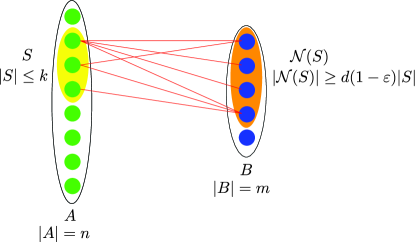
Figure 1: A $(k,\epsilon)$-expander. In this example, the green nodes correspond to $A$, the blue nodes correspond to $B$, the yellow oval corresponds to the set $S\subset A$, and the orange oval corresponds to the set ${\cal N}(S)\subset B$. There are three colliding edges.

Expanders have been recently proposed as a means of constructing efficient compressed sensing algorithms [15, 18, 19, 22]. In particular, it has been shown that any $n$-dimensional vector that is $k$-sparse can be fully recovered using $O\left(k\log\left(\frac{n}{k}\right)\right)$ measurements in $O\left(n\log\left(\frac{n}{k}\right)\right)$ time [15, 19]. It has been also shown that, even in the presence of noise in the measurements, if the noise vector has low $\ell_{1}$ norm, expander-based algorithms can approximately recover any $k$-sparse signal [18, 19, 16]. One reason why expander graphs are good sensing candidates is that the adjacency matrix of any $(k,\epsilon)$-expander almost preserves the $\ell_{1}$ norm of any $k$-sparse vector [18]. In other words, if the adjacency matrix of an expander is used for measurement, then the $\ell_{1}$ distance between two sufficiently sparse signals is preserved by measurement. This property is known as the “Restricted Isometry Property for $\ell_{1}$ norms” or the “RIP-1” property. Berinde et al. have shown that this condition is sufficient for sparse recovery using $\ell_{1}$ minimization [18].

The precise statement of the RIP-1 property, whose proof can be found in [15], goes as follows:

Lemma II.4 (RIP-1 property of the expander graphs).

Let ${F}$ be the $m\times n$ adjacency matrix of a $(k,\epsilon)$ expander graph $G$. Then for any $k$-sparse vector $x\in\mathbb{R}^{n}$ we have:

$$(1-2\epsilon)d\|x\|_{1}\leq\|{F}x\|_{1}\leq d\|x\|_{1}$$ (1)

The following proposition is a direct consequence of the above RIP-1 property. It states that if, for any almost $k$-sparse vector $u$, there exists a vector $v$ whose $\ell_{1}$ norm is close to that of $u$, and if ${F}v$ approximates ${F}u$, then $v$ also approximates $u$. Our results of Section III exploit the fact that the proposed MAP decoding algorithm outputs a vector satisfying the two conditions above, and hence approximately recovers the desired signal.

Proposition II.5.

Let ${F}$ be the adjacency matrix of a $(2k,\epsilon)$-expander and $u,v$ be two vectors in $\mathbb{R}^{n}$, such that

$$\|u\|_{1}\geq\|v\|_{1}-\Delta$$

for some $\Delta>0$. Then $\|u-v\|_{1}$ is upper-bounded by

$$\|u-v\|_{1}\leq\frac{1-2\epsilon}{1-6\epsilon}\left(2\sigma_{k}(u)+\Delta\right)+\frac{2}{d(1-6\epsilon)}\|{F}u-{F}v\|_{1}.$$

In particular, if we let $\epsilon=1/16$, then we get the bound

$$\|u-v\|_{1}\leq 4\sigma_{k}(u)+\frac{4}{d}\|{F}u-{F}v\|_{1}+2\Delta.$$

Proof:

See Appendix B.∎

For future convenience, we will introduce the following piece of notation. Given $n$ and $1\leq k\leq n/4$, we will denote by $G_{k,n}$ a $(2k,1/16)$-expander with left set size $n$ whose existence is guaranteed by Proposition II.2. Then $G_{k,n}=(A,B,E)$ has

$$|A|=n,\quad|B|=m=O(k\log(n/k)),\quad d=O(\log(n/k)).$$

III Compressed sensing in the presence of Poisson Noise

III-A Problem statement

We wish to recover an unknown vector $\theta^{*}\in\mathbb{R}_{+}^{n}$ of Poisson intensities from a measured vector $y\in\mathbb{Z}_{+}^{m}$, sensed according to the Poisson model

$$y\sim\text{Poisson}(\Phi\theta^{*}),$$ (2)

where $\Phi\in\mathbb{R}_{+}^{m\times n}$ is a positivity-preserving sensing matrix. That is, for each $j\in\{1,\ldots,m\}$, $y_{j}$ is sampled independently from a Poisson distribution with mean $(\Phi\theta^{*})_{j}$:

$${\mathbb{P}}_{\Phi\theta^{*}}(y)=\prod^{m}_{j=1}{\mathbb{P}}_{(\Phi\theta^{*})_{j}}(y_{j}),$$ (3)

where, for any $z\in\mathbb{Z}_{+}$ and $\lambda\in\mathbb{R}_{+}$, we have

$${\mathbb{P}}_{\lambda}(z)\stackrel{{\scriptstyle\scriptscriptstyle\triangle}}{{=}}\begin{cases}\displaystyle\frac{\lambda^{z}}{z!}e^{-\lambda}&\mbox{if }\lambda>0\\ 1_{\{z=0\}}&\mbox{otherwise}\end{cases},$$ (4)

where the $\lambda=0$ case is a consequence of the fact that

$$\lim_{\lambda\rightarrow 0}\frac{\lambda^{z}}{z!}e^{-\lambda}=1_{\{z=0\}}.$$

We assume that the $\ell_{1}$ norm of $\theta^{*}$ is known, $\|\theta^{*}\|_{1}=L$ (although later we will show that this assumption can be relaxed). We are interested in designing a sensing matrix $\Phi$ and an estimator $\hat{{\theta}}=\hat{{\theta}}(y)$, such that $\theta^{*}$ can be recovered with small expected $\ell_{1}$ risk

$$R\left(\hat{{\theta}},\theta^{*}\right)\stackrel{{\scriptstyle\scriptscriptstyle\triangle}}{{=}}{\mathbb{E}}_{\Phi\theta^{*}}\|\hat{{\theta}}-\theta^{*}\|_{1},$$

where the expectation is taken w.r.t. the distribution ${\mathbb{P}}_{\Phi\theta^{*}}$.

III-B The proposed estimator and its performance

To recover $\theta^{*}$, we will use a penalized Maximum Likelihood Estimation (pMLE) approach. Let us choose a convenient $1\leq k\leq n/4$ and take $\Phi$ to be the normalized adjacency matrix of the expander $G_{k,n}$ (cf. Section II for definitions): ${\Phi}\stackrel{{\scriptstyle\scriptscriptstyle\triangle}}{{=}}{F}/d$. Moreover, let us choose a finite or countable set $\Theta_{L}$ of candidate estimators ${\theta}\in\mathbb{R}_{+}^{n}$ with $\|{\theta}\|_{1}\leq L$, and a penalty ${\rm pen}:\Theta_{L}\to\mathbb{R}_{+}$ satisfying the Kraft inequality

$$\sum_{{\theta}\in\Theta_{L}}e^{-{\rm pen}({\theta})}\leq 1.$$ (5)

For instance, we can impose less penalty on sparser signals or construct a penalty based on any other prior knowledge about the underlying signal.

With these definitions, we consider the following penalized maximum likelihood estimator (pMLE):

$$\hat{{\theta}} \stackrel{{\scriptstyle\scriptscriptstyle\triangle}}{{=}}\operatornamewithlimits{argmin}_{{\theta}\in\Theta_{L}}\left[-\log{\mathbb{P}}_{{\Phi}{\theta}}({y})+2\,{\rm pen}({\theta})\right]$$ (6)

One way to think about the procedure in (6) is as a Maximum a posteriori Probability (MAP) algorithm over the set of estimates $\Theta_{L}$, where the likelihood is computed according to the Poisson model (4) and the penalty function corresponds to a negative log prior on the candidate estimators in $\Theta_{L}$.

Our main bound on the performance of the pMLE is as follows:

Theorem III.1.

Let ${\Phi}$ be the normalized adjacency matrix of $G_{k,n}$, let $\theta^{*}\in\mathbb{R}_{+}^{n}$ be the original signal compressively sampled in the presence of Poisson noise, and let $\hat{{\theta}}$ be obtained through (6). Then

$$R\left(\hat{{\theta}},\theta^{*}\right)\leq 4\sigma_{k}(\theta^{*})$$

$$\qquad+8\sqrt{L\min_{{\theta}\in\Theta_{L}}\left[\mbox{KL}({\mathbb{P}}_{{\Phi}\theta^{*}}\parallel{\mathbb{P}}_{{\Phi}{\theta}})+2\,{\rm pen}({\theta})\right]},$$ (7)

where

$$\mbox{KL}({\mathbb{P}}_{g}\|{\mathbb{P}}_{h})\stackrel{{\scriptstyle\scriptscriptstyle\triangle}}{{=}}\sum_{y\in\mathbb{Z}_{+}^{m}}{\mathbb{P}}_{g}(y)\log\frac{{\mathbb{P}}_{g}(y)}{{\mathbb{P}}_{h}(y)}$$

is the Kullback–Leibler divergence (relative entropy) between ${\mathbb{P}}_{g}$ and ${\mathbb{P}}_{h}$ [25].

Proof:

Since $\hat{{\theta}}\in\Theta_{L}$, we have $L=\|\theta^{*}\|_{1}\geq\|\hat{{\theta}}\|_{1}$. Hence, using Proposition II.5 with $\Delta=0$, we can write

$$\|\theta^{*}-\hat{{\theta}}\|_{1}\leq 4\sigma_{k}(\theta^{*})+4\|{\Phi}(\theta^{*}-\hat{{\theta}})\|_{1}.$$

Taking expectations, we obtain

$$R\left(\hat{{\theta}},\theta^{*}\right) \leq 4\sigma_{k}(\theta^{*})+4{\mathbb{E}}_{{\Phi}\theta^{*}}\|{\Phi}(\theta^{*}-\hat{{\theta}})\|_{1}$$

$$\leq 4\sigma_{k}(\theta^{*})+4\sqrt{{\mathbb{E}}_{{\Phi}\theta^{*}}\|{\Phi}(\theta^{*}-\hat{{\theta}})\|^{2}_{1}}$$ (8)

where the second step uses Jensen’s inequality. Using Lemmas C.1 and C.2 in Appendix C, we have

$${\mathbb{E}}_{{\Phi}\theta^{*}}\|{\Phi}(\theta^{*}-\hat{{\theta}})\|^{2}_{1}\leq 4L\min_{{\theta}\in\Theta_{L}}\left[\mbox{KL}({\mathbb{P}}_{{\Phi}\theta^{*}}\parallel{\mathbb{P}}_{{\Phi}{\theta}})+2\,{\rm pen}({\theta})\right]$$

Substituting this into (8), we obtain (7). ∎

The bound of Theorem III.1 is an oracle inequality: it states that the $\ell_{1}$ error of $\hat{{\theta}}$ is (up to multiplicative constants) the sum of the $k$-term approximation error of $\theta^{*}$ plus $\sqrt{L}$ times the minimum penalized relative entropy error over the set of candidate estimators $\Theta_{L}$. The first term in (7) is smaller for sparser $\theta^{*}$, and the second term is smaller when there is a ${\theta}\in\Theta_{L}$ which is simultaneously a good approximation to $\theta^{*}$ (in the sense that the distributions ${\mathbb{P}}_{\Phi\theta^{*}}$ and ${\mathbb{P}}_{\Phi{\theta}}$ are close) and has a low penalty.

Remark III.2.

So far we have assumed that the $\ell_{1}$ norm of $\theta^{*}$ is known a priori. If this is not the case, we can still estimate it with high accuracy using noisy compressive measurements. Observe that, since each measurement $y_{j}$ is a Poisson random variable with mean $\left(\Phi\theta^{*}\right)_{j}$, $\sum_{j}y_{j}$ is Poisson with mean $\|\Phi\theta^{*}\|_{1}$. Therefore, $\sqrt{\sum_{j}y_{j}}$ is approximately normally distributed with mean $\approx\sqrt{\|\Phi\theta^{*}\|_{1}}$ and variance $\approx\frac{1}{4}$ [26, Sec. 6.2]. Hence, Mill’s inequality [27, Thm. 4.7] guarantees that, for every positive $t$,

$$\Pr\left[\left|\sqrt{\sum_{j}y_{j}}-\sqrt{\|\Phi\theta^{*}\|_{1}}\right|>t\right]\lesssim\frac{e^{-2t^{2}}}{\sqrt{2\pi}t},$$

where $\lesssim$ is meant to indicate the fact that this is only an approximate bound, with the approximation error controlled by the rate of convergence in the central limit theorem. Now we can use the RIP-1 property of the expander graphs obtain the estimates

$$\left(\sqrt{\sum_{j}y_{j}}-t\right)^{2}\leq\|\Phi\theta^{*}\|_{1}\leq\|\theta^{*}\|_{1},$$

and

$$\frac{\left(\sqrt{\sum_{j}y_{j}}+t\right)^{2}}{(1-2\epsilon)}\geq\frac{\|\Phi\theta^{*}\|_{1}}{(1-2\epsilon)}\geq\|\theta^{*}\|_{1}$$

that hold with (approximate) probability at least $1-(\sqrt{2\pi}t)^{-1}e^{-2t^{2}}$.

III-C A bound in terms of $\ell_{1}$ error

The bound of Theorem III.1 is not always useful since it bounds the $\ell_{1}$ risk of the pMLE in terms of the relative entropy. A bound purely in terms of $\ell_{1}$ errors would be more desirable. However, it is not easy to obtain without imposing extra conditions either on $\theta^{*}$ or on the candidate estimators in $\Theta_{L}$. This follows from the fact that the divergence $\mbox{KL}({\mathbb{P}}_{\Phi\theta^{*}}\|{\mathbb{P}}_{\Phi\theta})$ may take the value $+\infty$ if there exists some $y$ such that ${\mathbb{P}}_{\Phi\theta}(y)=0$ but ${\mathbb{P}}_{\Phi\theta^{*}}(y)>0$.

One way to eliminate this problem is to impose an additional requirement on the candidate estimators in $\Theta_{L}$: There exists some $c>0$, such that

$$\Phi{\theta}\succeq c,\qquad\forall{\theta}\in\Theta_{L}$$ (9)

Under this condition, we will now develop a risk bound for the pMLE purely in terms of the $\ell_{1}$ error.

Theorem III.3.

Suppose that all the conditions of Theorem III.1 are satisfied. In addition, suppose that the set $\Theta_{L}$ satisfies the condition (9). Then

$$R\left(\hat{{\theta}},\theta^{*}\right)\leq 4\sigma_{k}(\theta^{*})+8\sqrt{L\min_{{\theta}\in\Theta_{L}}\left[\frac{\|\theta^{*}-{\theta}\|^{2}_{1}}{c}+2\,{\rm pen}({\theta})\right]}.$$ (10)

Proof:

Using Lemma C.3 in Appendix C, we get the bound

$$\mbox{KL}({\mathbb{P}}_{\Phi\theta^{*}}\|{\mathbb{P}}_{\Phi\theta})\leq\frac{1}{c}\|\theta^{*}-{\theta}\|^{2}_{1},\qquad\forall{\theta}\in\Theta_{L}.$$

Substituting this into Eq. (7), we get (10). ∎

Remark III.4.

Because every ${\theta}\in\Theta_{L}$ satisfies $\|{\theta}\|_{1}\leq L$, the constant $c$ cannot be too large. In particular, if (9) holds, then for every ${\theta}\in\Theta_{L}$ we must have

$$\|\Phi{\theta}\|_{1}\geq m\min_{j}(\Phi{\theta})_{j}\geq mc.$$

On the other hand, by the RIP-$1$ property we have $\|\Phi{\theta}\|_{1}\leq\|{\theta}\|_{1}\leq L$. Thus, a necessary condition for (9) to hold is $c\leq L/m$. Since $m=O(k\log(n/k))$, the best risk we may hope to achieve under some condition like (9) is on the order of

$$R\left(\hat{{\theta}},\theta^{*}\right)\leq 4\sigma_{k}(\theta^{*})$$

$$\qquad\qquad+C\sqrt{\min_{{\theta}\in\Theta_{L}}\left[k\log(n/k)\|{\theta}-\theta^{*}\|^{2}_{1}+L\,{\rm pen}({\theta})\right]}$$ (11)

for some constant $C$, e.g., by choosing $c\propto\frac{L}{k\log(n/k)}$. Effectively, this means that, under the positivity condition (9), the $\ell_{1}$ error of $\hat{{\theta}}$ is the sum of the $k$-term approximation error of $\theta^{*}$ plus $\sqrt{m}=\sqrt{k\log(n/k)}$ times the best penalized $\ell_{1}$ approximation error. The first term in (11) is smaller for sparser $\theta^{*}$, and the second term is smaller when there is a ${\theta}\in\Theta_{L}$ which is simultaneously a good $\ell_{1}$ approximation to $\theta^{*}$ and has a low penalty.

III-D Empirical performance

Here we present a simulation study that validates our method. In this experiment, compressive Poisson observations are collected of a randomly generated sparse signal passed through the sensing matrix generated from an adjacency matrix of an expander. We then reconstruct the signal by utilizing an algorithm that minimizes the objective function in (6), and assess the accuracy of this estimate. We repeat this procedure over several trials to estimate the average performance of the method.

More specifically, we generate our length-$n$ sparse signal $\theta^{*}$ through a two-step procedure. First we select $k$ elements of $\{1,\ldots,n\}$ uniformly at random, then we assign these elements an intensity $I$. All other components of the signal are set to zero. For these experiments, we chose a length $n=\text{100,000}$ and varied the sparsity $k$ among three different choices of 100, 500, and 1,000 for two intensity levels $I$ of 10,000 and 100,000. We then vary the number $m$ of Poisson observations from 100 to 20,000 using an expander graph sensing matrix with degree $d=8$. Recall that the sensing matrix is normalized such that the total signal intensity is divided amongst the measurements, hence the seemingly high choices of $I$.

To reconstruct the signal, we utilize the SPIRAL-$\ell_{1}$ algorithm [28] which solves (6) when ${\rm pen}({\theta})=\tau\|{\theta}\|_{1}$. We design the algorithm to optimize over the continuous domain $\mathbb{R}_{+}^{n}$ instead of the discrete set $\Theta_{L}$. This is equivalent to the proposed pMLE formulation in the limit as the discrete set of estimates becomes increasingly dense in the set of all $\theta\in\mathbb{R}^{n}_{+}$ with $\|\theta\|_{1}\leq L$, i.e., we quantize this set on an ever finer scale, increasing the bit allotment to represent each $\theta$. In this high-resolution limit, the Kraft inequality requirement (5) on the penalty ${\rm pen}(\theta)$ will translate to $\int e^{-{\rm pen}(\theta)}d\theta<\infty$. If we select a penalty proportional to the negative log of a prior probability distribution for $\theta$, this requirement will be satisfied. From a Bayesian perspective, the $\ell_{1}$ penalty arises by assuming each component $\theta_{i}$ is drawn i.i.d. from a zero-mean Laplace prior $p(\theta_{i})=e^{-|\theta_{i}|/b}/2b$. Hence the regularization parameter $\tau$ is inversely related to the scale parameter $b$ of the prior, as a larger $\tau$ (smaller $b$) will promote solutions with more zero-valued components.

This relaxation results in a computationally tractable convex program over a continuous domain, albeit implemented on a machine with finite precision. The SPIRAL algorithm utilizes a sequence of quadratic subproblems derived by using a second-order Taylor expansion of the Poisson log-likelihood at each iteration. These subproblems are made easier to solve by using a separable approximation whereby the second-order Hessian matrix is approximated by a scaled identity matrix. For the particular case of the $\ell_{1}$ penalty, these subproblems can be solved quickly, exactly, and noniteratively by a soft-thresholding rule.

After reconstruction, we assess the estimate $\hat{{\theta}}$ according to the normalized $\ell_{1}$ error $\|\theta^{*}-\hat{{\theta}}\|_{1}/\|\theta^{*}\|_{1}$. We select the regularization weighting $\tau$ in the SPIRAL-$\ell_{1}$ algorithm to minimize this quantity for each randomly generated experiment indexed by $(I,k,m)$. To assure that the results are not biased in our favor by only considering a single random experiment for each $(I,k,m)$, we repeat this experiment several times. The averaged reconstruction accuracy over 10 trials is presented in Figure 2.

These results show that the proposed method is able to accurately estimate sparse signals when the signal intensity is sufficiently high; however, the performance of the method degrades for lower signal strengths. More interesting is the behavior as we vary the number of measurements. There is a clear phase transition where accurate signal reconstruction becomes possible, however the performance gently degrades with the number of measurements since there is a lower signal-to-noise ratio per measurement. This effect is more pronounced at lower intensity levels, as we more quickly enter the regime where only a few photons are collected per measurement. These findings support the error bounds developed in Section III-B.

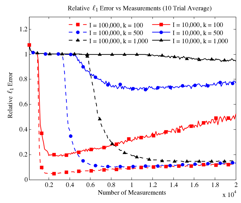
Figure 2: Average performance (as measured by the normalized $\ell_{1}$ error $\|\theta^{*}-\hat{{\theta}}\|_{1}/\|\theta^{*}\|_{1}$) for the proposed expander-based observation method for recovering sparse signals under Poisson noise. In this experiment, we sweep over a range of measurements and

consider a few sparsity ($k$) and intensity $(I)$ levels of the true signal.

IV Application: Estimating packet arrival rates

This section describes an application of the pMLE estimator of Section III: an indirect approach for reconstructing average packet arrival rates and instantaneous packet counts for a given number of streams (or flows) at a router in a communication network, where the arrivals of packets in each flow are assumed to follow a Poisson process. All packet counting must be done in hardware at the router, and any hardware implementation must strike a delicate balance between speed, accuracy, and cost. For instance, one could keep a dedicated counter for each flow, but, depending on the type of memory used, one could end up with an implementation that is either fast but expensive and unable to keep track of a large number of flows (e.g., using SRAMs, which have low access times, but are expensive and physically large) or cheap and high-density but slow (e.g., using DRAMs, which are cheap and small, but have longer access times) [29, 30].

However, there is empirical evidence [31, 32] that flow sizes in IP networks follow a power-law pattern: just a few flows (say, $10\%$) carry most of the traffic (say, $90\%$). Based on this observation, several investigators have proposed methodologies for estimating flows using a small number of counters by either (a) keeping track only of the flows whose sizes exceed a given fraction of the total bandwidth (the approach suggestively termed “focusing on the elephants, ignoring the mice”) [29] or (b) using sparse random graphs to aggregate the raw packet counts and recovering flow sizes using a message passing decoder [30].

We consider an alternative to these approaches based on Poisson CS, assuming that the underlying Poisson rate vector is sparse or approximately sparse — and, in fact, it is the approximate sparsity of the rate vector that mathematically describes the power-law behavior of the average packet counts. The goal is to maintain a compressed summary of the process sample paths using a small number of counters, such that it is possible to reconstruct both the total number of packets in each flow and the underlying rate vector. Since we are dealing here with Poisson streams, we would like to push the metaphor further and say that we are “focusing on the whales, ignoring the minnows.”

IV-A Problem formulation

We wish to monitor a large number $n$ of packet flows using a much smaller number $m$ of counters. Each flow is a homogeneous Poisson process (cf. [4] for details pertaining to Poisson processes and networking applications). Specifically, let $\lambda^{*}\in\mathbb{R}_{+}^{n}$ denote the vector of rates, and let $U$ denote the random process $U=\{U_{t}\}_{t\in\mathbb{R}_{+}}$ with sample paths in $\mathbb{Z}_{+}^{n}$, where, for each $i\in\{1,\ldots,n\}$, the $i$th component of $U$ is a homogeneous Poisson process with the rate of $\lambda_{i}$ arrivals per unit time, and all the component processes are mutually conditionally independent given $\lambda$.

The goal is to estimate the unknown rate vector $\lambda$ based on ${y}$. We will focus on performance bounds for power-law network traffic, i.e., for $\lambda^{*}$ belonging to the class

$$\Sigma_{\alpha,L_{0}}\stackrel{{\scriptstyle\scriptscriptstyle\triangle}}{{=}}\left\{\lambda\in\mathbb{R}_{+}^{n}:\|\lambda\|_{1}=L_{0};{\sigma_{k}(\lambda)=O(k^{-\alpha})}\right\}$$ (12)

for some $L_{0}>0$ and $\alpha\geq 1$, where the constant hidden in the $O(\cdot)$ notation may depend on $L_{0}$. Here, $\alpha$ is the power-law exponent that controls the tail behavior; in particular, the extreme regime $\alpha\to+\infty$ describes the fully sparse setting. As in Section III, we assume the total arrival rate $\|\lambda^{*}\|_{1}$ to be known (and equal to a given $L_{0}$) in advance, but this assumption can be easily dispensed with (cf. Remark III.2).

As before, we evaluate each candidate estimator $\widehat{\lambda}=\widehat{\lambda}(y)$ based on its expected $\ell_{1}$ risk,

$$R\left(\widehat{\lambda},\lambda^{*}\right)={\mathbb{E}}_{\lambda^{*}}\|\widehat{\lambda}-\lambda^{*}\|_{1}.$$

IV-B Two estimation strategies

We consider two estimation strategies. In both cases, we let our measurement matrix ${F}$ be the adjacency matrix of the expander $G_{k,n}$ for a fixed $k\leq n/4$ (see Section II for definitions). The first strategy, which we call the direct method, uses standard expander-based CS to construct an estimate of $\lambda^{*}$. The second is the pMLE strategy, which relies on the machinery presented in Section III and can be used when only the rates are of interest.

IV-B1 The direct method

In this method, which will be used as a “baseline” for assessing the performance of the pMLE, the counters are updated in discrete time, every $\tau$ time units. Let $x=\{x_{\nu}\}_{\nu\in\mathbb{Z}_{+}}$ denote the sampled version of $U$, where $x_{\nu}\stackrel{{\scriptstyle\scriptscriptstyle\triangle}}{{=}}U_{\nu\tau}$. The update takes place as follows. We have a binary matrix ${F}\in\{0,1\}^{m\times n}$, and at each time $\nu$ let ${y}_{\nu}={F}x_{\nu}$. In other words, ${y}$ is obtained by passing a sampled $n$-dimensional homogeneous Poisson process with rate vector $\lambda$ through a linear transformation ${F}$.

The direct method uses expander-based CS to obtain an estimate $\widehat{x}_{\nu}$ of $x_{\nu}$ from ${y}_{\nu}={F}x_{\nu}$, followed by letting

$$\widehat{\lambda}_{\nu}^{\rm dir}=\frac{\widehat{x}^{+}_{\nu}}{\nu\tau}.$$ (13)

This strategy is based on the observation that $x_{\nu}/(\nu\tau)$ is the maximum-likelihood estimator of $\lambda^{*}$. To obtain $\widehat{x}_{\nu}$, we need to solve the convex program

minimize $$\|u\|_{1}\qquad\text{ subject to }{F}u={y}_{\nu}$$

which can be cast as a linear program [33]. The resulting solution $\widehat{x}_{\nu}$ may have negative coordinates, hence the use of the $(\cdot)^{+}$ operation in (13). We then have the following result:

Theorem IV.1.

$$R\left(\widehat{\lambda}_{\nu}^{\rm dir},\lambda^{*}\right)\leq 4\sigma_{k}(\lambda^{*})+\frac{\|(\lambda^{*})^{1/2}\|_{1}}{\sqrt{\nu\tau}},$$ (14)

where $(\lambda^{*})^{1/2}$ is the vector with components $\sqrt{\lambda^{*}_{i}},\forall i$.

Remark IV.2.

Note that the error term in (14) is $O(1/\sqrt{\nu})$, assuming everything else is kept constant, which coincides with the optimal rate of the $\ell_{1}$ error decay in parametric estimation problems.

Proof:

We first observe that, by construction, $\widehat{x}_{\nu}$ satisfies the relations ${F}\widehat{x}_{\nu}={F}x_{\nu}$ and $\|\widehat{x}_{\nu}\|_{1}\leq\|x_{\nu}\|_{1}$. Hence,

$${\mathbb{E}}\|\widehat{x}_{\nu}-\nu\tau\lambda^{*}\|_{1} \leq{\mathbb{E}}\|\widehat{x}_{\nu}-x_{\nu}\|_{1}+{\mathbb{E}}\|x_{\nu}-\nu\tau\lambda^{*}\|_{1}$$

$$\leq 4{\mathbb{E}}\sigma_{k}(x_{\nu})+{\mathbb{E}}\|x_{\nu}-\nu\tau\lambda^{*}\|_{1}$$ (15)

where the first step uses the triangle inequality, while the second step uses Proposition II.5 with $\Delta=0$. To bound the first term in (15), let $S\subset\{1,\ldots,n\}$ denote the positions of the $k$ largest entries of $\lambda^{*}$. Then, by definition of the best $k$-term representation,

$$\sigma_{k}(x_{\nu})\leq\|x_{\nu}-x^{S}_{\nu}\|_{1}=\sum_{i\in S^{c}}|x_{\nu,i}|=\sum_{i\in S^{c}}x_{\nu,i}.$$

Therefore,

$${\mathbb{E}}\sigma_{k}(x_{\nu})\leq{\mathbb{E}}\left[\sum_{i\in S^{c}}x_{\nu,i}\right]=\nu\tau\sum_{i\in S^{c}}\lambda_{i}^{*}\equiv\nu\tau\sigma_{k}(\lambda^{*}).$$

To bound the second term, we can use concavity of the square root, as well as the fact that each $x_{\nu,i}\sim{\rm Poisson}(\nu\tau\lambda^{*}_{i})$, to write

$${\mathbb{E}}\|x_{\nu}-\nu\tau\lambda^{*}\|_{1} ={\mathbb{E}}\left[\sum^{N}_{i=1}|x_{n,i}-\nu\tau\lambda^{*}_{i}|\right]$$

$$={\mathbb{E}}\left[\sum^{N}_{i=1}\sqrt{(x_{n,i}-\nu\tau\lambda^{*}_{i})^{2}}\right]$$

$$\leq\sum^{n}_{i=1}\sqrt{{\mathbb{E}}(x_{\nu,i}-\nu\tau\lambda^{*}_{i})^{2}}=\sum^{n}_{i=1}\sqrt{\nu\tau\lambda^{*}_{i}}.$$

Now, it is not hard to show that $\|\widehat{x}^{+}_{\nu}-\nu\tau\lambda^{*}\|_{1}\leq\|\widehat{x}_{\nu}-\nu\tau\lambda^{*}\|_{1}$. Therefore,

$$R\left(\widehat{\lambda}_{\nu}^{\rm dir},\lambda^{*}\right) \leq\frac{{\mathbb{E}}\|\widehat{x}_{\nu}-\nu\tau\lambda^{*}\|_{1}}{\nu\tau}\leq 4\sigma_{k}(\lambda^{*})+\frac{\|(\lambda^{*})^{1/2}\|_{1}}{\sqrt{\nu\tau}},$$

which proves the theorem. ∎

IV-B2 The penalized MLE approach

In the penalized MLE approach the counters are updated in a slightly different manner. Here the counters are still updated in discrete time, every $\tau$ time units; however, each counter $i\in\left\{1,\cdots,m\right\}$ is updated at times $\left(\nu\tau+\frac{i}{m}\tau\right)_{\nu\in\mathbb{Z}_{+}}$, and only aggregates the packets that have arrived during the time period $\left[\nu\tau+\frac{i-1}{m}\tau,\nu\tau+\frac{i}{m}\tau\right)$. Therefore, in contrast to the direct method, here each arriving packet is registered by at most one counter. Furthermore, since the packets arrive according to a homogeneous Poisson process, conditioned on the vector $\lambda^{*}$, the values measured by distinct counters are independent. Therefore, the vector of counts at time $\nu$ obeys

$$y_{\nu}\sim\text{Poisson}({\Phi}\theta^{*})\qquad\text{where}\qquad\theta^{*}=\frac{\nu\tau d}{m}\lambda^{*}$$

which is precisely the sensing model we have analyzed in Section III.

Now assume that the total average arrival rate $\|\lambda^{*}\|_{1}=L_{0}$ is known. Let $\Lambda$ be a finite or a countable set of candidate estimators with $\|\lambda\|_{1}\leq L_{0}$ for all $\lambda\in\Lambda$, and let ${\rm pen}(\cdot)$ be a penalty functional satisfying the Kraft inequality over $\Lambda$. Given $\nu$ and $\tau$, consider the scaled set

$$\Lambda_{\nu,\tau}\stackrel{{\scriptstyle\scriptscriptstyle\triangle}}{{=}}\frac{\nu\tau d}{m}\Lambda\equiv\left\{\frac{\nu\tau d}{m}\lambda:\lambda\in\Lambda\right\}$$

with the same penalty function, ${\rm pen}\left(\frac{\nu\tau d}{m}\lambda\right)={\rm pen}(\lambda)$ for all $\lambda\in\Lambda$. We can now apply the results of Section III. Specifically, let

$$\widehat{\lambda}^{\rm pMLE}_{\nu}\stackrel{{\scriptstyle\scriptscriptstyle\triangle}}{{=}}\frac{m\,\hat{{\theta}}}{\nu\tau d},$$

where $\hat{{\theta}}$ is the corresponding pMLE estimator obtained according to (6). The following theorem is a consequence of Theorem III.3 and the remark following it:

Theorem IV.3.

If the set $\Lambda$ satisfies the strict positivity condition (9), then there exists some absolute constant $C>0$, such that

$$R\left(\widehat{\lambda}^{\rm pMLE}_{\nu},\lambda^{*}\right)\leq 4\sigma_{k}(\lambda^{*})$$

$$\qquad+C\sqrt{\min_{\lambda\in\Lambda}\left[k\log(n/k)\|\lambda-\lambda^{*}\|^{2}_{1}+\frac{k\,L_{0}\,{\rm pen}(\lambda)}{\nu\tau}\right]}.$$ (16)

We now develop risk bounds under the power-law condition. To this end, let us suppose that $\lambda^{*}$ is a member of the power-law class $\Sigma_{L_{0},\alpha}$ defined in (12). Fix a small positive number $\delta$, such that $L_{0}/\sqrt{\delta}$ is an integer, and define the set

$$\Lambda\stackrel{{\scriptstyle\scriptscriptstyle\triangle}}{{=}}\left\{\lambda\in\mathbb{R}_{+}^{n}:\|\lambda\|_{1}\leq L_{0};\lambda_{i}\in\{s\sqrt{\delta}\}^{L_{0}/\sqrt{\delta}}_{s=0},\forall i\right\}$$

These will be our candidate estimators of $\lambda^{*}$. We can define the penalty function ${\rm pen}(\lambda)\asymp\|\lambda\|_{0}\log(\delta^{-1})$. For any $\lambda\in\Sigma_{\alpha,L_{0}}$ and any $1\leq r\leq n$ we can find some $\lambda^{(r)}\in\Lambda$, such that $\|\lambda^{(r)}\|_{0}\asymp r$ and

$$\|\lambda-\lambda^{(r)}\|^{2}_{1}\asymp r^{-2\alpha}+r\,\delta.$$

Here we assume that $\delta$ is sufficiently small, so that the penalty term $\frac{k\,r\log(\delta^{-1})}{\nu\tau}$ dominates the quantization error $r\,\delta$. In order to guarantee that the penalty function satisfies Kraft’s inequality, we need to ensure that

$$\sum_{r=1}^{n}\sum_{\begin{subarray}{c}\lambda^{(r)}\in\Lambda\\ \|\lambda^{(r)}\|_{0}=r\end{subarray}}\delta^{r}\leq 1.$$

For every fixed $r$, there are exactly ${n\choose r}$ subspaces of dimension $r$, and each subspace contains exactly $\left(\frac{L_{0}}{\sqrt{\delta}}\right)^{r}$ distinct elements of $\Lambda$. Therefore, as long as

$$\delta\leq\left(2n\,L_{0}\right)^{-2},$$ (17)

then

$$\sum_{r=1}^{n}{n\choose r}\left(L_{0}\,\sqrt{\delta}\right)^{r}\leq\sum_{r=0}^{n}\left(n\,L_{0}\,\sqrt{\delta}\right)^{r}\leq\sum_{r=1}^{n}\frac{1}{2^{r}}\leq 1,$$

and Kraft’s inequality is satisfied.

Using the fact that $k\log(n/k)=O(kd)$, we can bound the minimum over $\lambda\in\Lambda$ in (16) from above by

$$\min_{1\leq r\leq n}\left[kdr^{-2\alpha}+\frac{r\,k\log(\delta^{-1})}{\nu\tau}\right]$$

$$\qquad=O\left(k\,d^{\frac{1}{2\alpha+1}}\right)\left(\frac{\log(\delta^{-1})}{\nu\tau}\right)^{\frac{2\alpha}{2\alpha+1}}$$

$$\qquad=O\left(k\,d^{\frac{1}{2\alpha+1}}\right)\left(\frac{\log n}{\nu\tau}\right)^{\frac{2\alpha}{2\alpha+1}}$$

We can now particularize Theorem IV.3 to the power-law case:

Theorem IV.4.

$$\sup_{\lambda^{*}\in\Sigma_{\alpha,L_{0}}}R\left(\widehat{\lambda}^{\rm pMLE}_{\nu},\lambda^{*}\right)$$

$$\quad=O(k^{-\alpha})+O\left(k^{\frac{1}{2}}\,d^{\frac{1}{4\alpha+2}}\right)\left(\frac{\log n}{\nu\tau}\right)^{\frac{\alpha}{2\alpha+1}},$$

where the constants implicit in the $O(\cdot)$ notation depend on $L_{0}$ and $\alpha$.

Note that the risk bound here is slightly worse than the benchmark bound of Theorem IV.1. However, it should be borne in mind that this bound is based on Theorem III.3, rather than on the potentially much tighter oracle inequality of Theorem III.1, since our goal was to express the risk of the pMLE purely in terms of the $\ell_{1}$ approximation properties of the power-law class $\Sigma_{\alpha,L_{0}}$. In general, we will expect the actual risk of the pMLE to be much lower than what the conservative bound of Theorem IV.4 predicts. Indeed, as we will see in Section IV-D, the pMLE approach obtains higher empirical accuracy than the direct method. But first we show how the pMLE can be approximated efficiently with proper preprocessing of the observed counts ${y}_{\nu}$ based on the structure of $G_{k,n}$.

IV-C Efficient pMLE approximation

In this section we present an efficient algorithm for approximating the pMLE estimate. The algorithm consists of two phases: (1) first, we preprocess ${y}_{\nu}$ to isolate a subset $A_{1}$ of $A=\{1,\ldots,n\}$ which is sufficiently small and is guaranteed to contain the locations of the $k$ largest entries of $\lambda^{*}$ (the whales); (2) then we construct a set $\Lambda$ of candidate estimators whose support sets lie in $A_{1}$, together with an appropriate penalty, and perform pMLE over this reduced set.

The success of this approach hinges on the assumption that the magnitude of the smallest whale is sufficiently large compared to the magnitude of the largest minnow. Specifically, we make the following assumption: Let $S\subset A$ contain the locations of the $k$ largest coordinates of $\lambda^{*}$. Then we require that

$$\min_{i\in S}\lambda^{*}_{i}>9D\left\|\lambda^{*}-{\lambda^{*}}^{(k)}\right\|_{\infty}.$$ (18)

Recall that $D=O\left(\frac{nd}{m}\right)=O\left(\frac{n}{k}\right)$ is the right degree of the expander graph. One way to think about (18) is in terms of a signal-to-noise ratio, which must be strictly larger than $9\,D$. We also require $\nu\tau$ to be sufficiently large, so that

$$\frac{\nu\tau}{m}\,D\left\|\lambda^{*}-{\lambda^{*}}^{(k)}\right\|_{\infty}\geq\frac{\log\left(mn\right)}{2}.$$ (19)

Finally, we perturb our expander a bit as follows: choose an integer $k^{\prime}>0$ so that

$$k^{\prime}\geq\max\left\{\frac{16(kd+1)}{15d},2k\right\}.$$ (20)

Then we replace our original $(2k,1/16)$-expander $G_{k,n}$ with left-degree $d$ with a $(k^{\prime},1/16)$-expander $G^{\prime}_{k^{\prime},n}$ with the same left degree.The resulting procedure, displayed below as Algorithm 1, has the following guarantees:

Algorithm 1 Efficient pMLE approximation algorithm

Input: Measurement vector ${y}_{\nu}$, and the sensing matrix ${F}$. Output: An approximation $\widehat{\lambda}$

  Let $B_{1}$ consist of the locations of the $kd$ largest elements of ${y}_{\nu}$ and let $B_{2}=B\backslash B_{1}$.

  Let $A_{2}$ contain the set of all variable nodes that have at least one neighbor in $B_{2}$ and let $A_{1}\nobreak=A\backslash A_{2}$.

  Construct a candidate set of estimators $\Lambda$ with support in $A_{1}$ and a penalty ${\rm pen}(\cdot)$ over $\Lambda$.

  Output the pMLE $\widehat{\lambda}$.

Theorem IV.5.

Suppose the assumptions (18), (19), and (20) hold. Then with probability at least $1-\frac{1}{n}$ the set $A_{1}$ constructed by Algorithm 1 has the following properties: (1) $S\subset A_{1}$; (2) $|A_{1}|\leq kd$; (3) $A_{1}$ can be found in time $O(m\log m+nd)$.

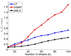
(a) $\alpha=1$

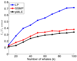
(b) $\alpha=1.5$

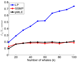
(c) $\alpha=2$

Figure 3: Relative $\ell_{1}$ error as a function of number of whales $k$, for $\ell_{1}$-magic (LP), SSMP and pMLE for different choices of the power-law exponent $\alpha$. The number of flows $n=5000$, the number of counters ${m}=800$, and the number of updates is $40$.

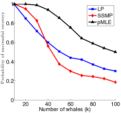
(a) $\alpha=1$

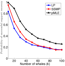
(b) $\alpha=1.5$

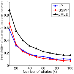
(c) $\alpha=2$

Figure 4: Probability of successful support recovery as a function of number of whales $k$, for $\ell_{1}$-magic (LP), SSMP and pMLE for different choices of the power-law exponent $\alpha$. The number of flows $n=5000$, the number of counters ${m}=800$, and the number of updates is $40$.

Proof:

(1) First fix a measurement node $j\in B$. Recall that ${y}_{\nu,j}$ is a Poisson random variable with mean $\frac{\nu\tau}{m}\left({F}\lambda^{*}\right)_{j}$. By the same argument as in Remark III.2, $\sqrt{{y}_{\nu,j}}$ is approximately normally distributed with mean $\approx\sqrt{\frac{\nu\tau}{m}\left({F}\lambda^{*}\right)_{j}}$, and with variance $\approx\frac{1}{4}$. Hence, it follows from Mill’s inequality and the union bound that for every positive $t$

$$\Pr\left[\exists j:\left|\sqrt{{y}_{\nu,j}}-\sqrt{\frac{\nu\tau}{m}\left({F}\lambda^{*}\right)_{j}}\right|>t\right]\lesssim\frac{me^{-2t^{2}}}{\sqrt{2\pi}t}.$$

If $j$ is a neighbor of $S$, then $\left({F}\lambda^{*}\right)_{j}\geq\min_{i\in S}\lambda^{*}_{i}$; whereas if $j$ is not connected to $S$, then $\left({F}\lambda^{*}\right)_{j}\leq D\left\|\lambda^{*}-{\lambda^{*}}^{(k)}\right\|_{\infty}$. Hence, by setting $t=\sqrt{\frac{\log\left(mn\right)}{2}}$ (where w.l.o.g. we assume that $t\geq 1$), we conclude that, with probability at least $1-\frac{1}{n}$, for every measurement node $j$ the following holds:

• If $j$ is a neighbor of $S$, then

  $$\sqrt{{y}_{\nu,j}}\geq\sqrt{\frac{\nu\tau}{m}\min_{i\in S}\lambda^{*}_{i}}-\sqrt{\frac{\log\left(mn\right)}{2}}.$$

• If $j$ is not connected to $S$, then

  $$\sqrt{{y}_{\nu,j}}\leq\sqrt{\frac{\nu\tau}{m}D\left\|\lambda^{*}-{\lambda^{*}}^{(k)}\right\|_{\infty}}+\sqrt{\frac{\log\left(mn\right)}{2}}.$$

Consequently, by virtue of (18) and (19), with probability at least $1-\frac{1}{n}$ every element of ${y}_{\nu}$ that is a neighbor of $S$ has larger magnitude than every element of ${y}_{\nu}$ that is not a neighbor of $S$.

(2) Suppose, to the contrary, that $|A_{1}|>kd$. Let $A^{\prime}_{1}\subseteq A_{1}$ be any subset of size $kd+1$. Now, Lemma 3.6 in [34] states that, provided $\epsilon\leq 1-1/d$, then every $(\ell,\epsilon)$-expander with left degree $d$ is also a $(\ell(1-\epsilon)d,1-1/d)$-expander with left degree $d$. We apply this result to our $(k^{\prime},1/16)$-expander, where $k^{\prime}$ satisfies (20), to see that it is also a $(kd+1,1-1/d)$-expander. Therefore, for the set $A^{\prime}_{1}$ we must have $|{\mathcal{N}}(A^{\prime}_{1})|\geq|A^{\prime}_{1}|=kd+1$. On the other hand, ${\mathcal{N}}(A^{\prime}_{1})\subset B_{1}$, so $|{\mathcal{N}}(A^{\prime}_{1})|\leq kd$. This is a contradiction, hence we must have $|A_{1}|\leq kd$.

(3) Finding the sets $B_{1}$ and $B_{2}$ can be done in $O(m\log m)$ time by sorting ${y}_{\nu}$. The set $A_{1}$ can then can be found in time $O(nd)$, by sequentially eliminating all nodes connected to each node in $B_{2}$. ∎

Having identified the set $A_{1}$, we can reduce the pMLE optimization only to those candidates whose support sets lie in $A_{1}$. More precisely, if we originally start with a sufficiently rich class of estimators $\tilde{\Lambda}$, then the new feasible set can be reduced to

$$\Lambda\stackrel{{\scriptstyle\scriptscriptstyle\triangle}}{{=}}\left\{\lambda\in\tilde{\Lambda}:{\rm Supp}(\lambda)\subset A_{1}\right\}.$$

Hence, by extracting the set $A_{1}$, we can significantly reduce the complexity of finding the pMLE estimate. If $|\Lambda|$ is small, the optimization can be performed by brute-force search in $O(|\Lambda|)$ time. Otherwise, since $|A_{1}|\leq kd$, we can use the quantization technique from the preceding section with quantizer resolution $\sqrt{\delta}$ to construct a $\Lambda$ of size at most $(L_{0}/\sqrt{\delta})^{kd}$. In this case, we can even assign the uniform penalty

$${\rm pen}(\lambda)=\log|\Lambda|=O\left(k\log(n/k)\log(\delta^{-1})\right),$$

which amounts to a vanilla MLE over $\Lambda$.

IV-D Empirical performance

Here we compare penalized MLE with $\ell_{1}$-magic [35], a universal $\ell_{1}$ minimization method, and with SSMP [36], an alternative method that employs combinatorial optimization. $\ell_{1}$-magic and SSMP both compute the “direct” estimator. The pMLE estimate is computed using Algorithm 1 above. For the ease of computation, the candidate set $\Lambda$ is approximated by the convex set of all positive vectors with bounded $\ell_{1}$ norm, and the CVX package [37, 38] is used to directly solve the pMLE objective function with ${\rm pen}(\theta)=\|\theta\|_{1}$.

Figures 3(a) through 5(b) report the results of numerical experiments, where the goal is to identify the $k$ largest entries in the rate vector from the measured data. Since a random graph is, with overwhelming probability, an expander graph, each experiment was repeated $30$ times using independent sparse random graphs with $d=8$.

We also used the following process to generate the rate vector. First, given the power-law exponent $\alpha$, the magnitudes of the $k$ whales were chosen according to a power-law distribution with parameter $\alpha$. The positions of the $k$ whales were then chosen uniformly at random. Finally the $n-k$ minnows were sampled independently from a ${\cal N}(0,10^{-6})$ distribution (negative samples were replaced by their absolute values). Thus, given the locations of the $k$ whales, their magnitudes decay according to a truncated power law (with the cut-off at $k$), while the magnitudes of the minnows represent a noisy background.

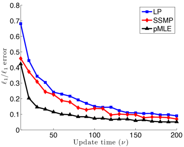
(a) Relative $\ell_{1}$ error as a function of number of updates $\nu$.

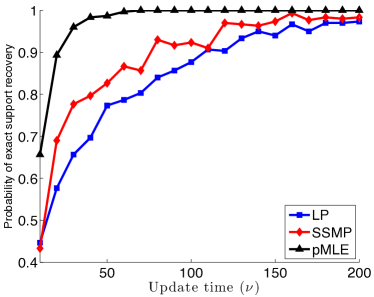
(b) Probability of successful support recovery as a function of number of updates $\nu$.

Figure 5: Performance of $\ell_{1}$-magic, SSMP and pMLE algorithms as a function of the number of updates $\nu$. The number of flows $n=5000$, the number of counters ${m}=800$, and the number of whales is $k=30$. There are $k$ whales whose magnitudes are assigned according to a power-law distribution with $\alpha=1$, and the remaining entries are minnows with magnitudes determined by a ${\cal N}(0,10^{-6})$ random variable.

Figure 3 shows the relative $\ell_{1}$ error ($\|\lambda-\widehat{\lambda}_{\nu}\|_{1}/\|\lambda\|_{1}$) of the three above algorithms as a function of $k$. Note that in all cases $\alpha=1$, $\alpha=1.5$, and $\alpha=2$, the pMLE algorithm provides lower $\ell_{1}$ errors. Similarly, Figure 4 reports the probability of exact recovery as a function of $k$. Again, it turns out that in all three cases the pMLE algorithm has higher probability of exact support recovery compared to the two direct algorithms.

We also analyzed the impact of changing the number of updates on the accuracy of the three above algorithms. The results are demonstrated in Figure 5. Here we fixed the number of whales to $k=30$, and changed the number of updates from $10$ to $200$. It turned out that as the number of updates $\nu$ increases, the relative $\ell_{1}$ errors of all three algorithms decrease and their probability of exact support recovery consistently increase. Moreover, the pMLE algorithm always outperforms the $\ell_{1}$-magic (LP), and SSMP algorithms.

V Conclusions

In this paper we investigated expander-based sensing as an alternative to dense random sensing in the presence of Poisson noise. Even though the Poisson model is essential in some applications, it presents several challenges as the noise is not bounded, or even as concentrated as Gaussian noise, and is signal-dependent. Here we proposed using normalized adjacency matrices of expander graphs as an alternative construction of sensing matrices, and we showed that the binary nature and the RIP-1 property of these matrices yield provable consistency for a MAP reconstruction algorithm.

The compressed sensing algorithms based on Poisson observations and expander-graph sensing matrices provide a useful mechanism for accurately and robustly estimating a collection of flow rates with relatively few counters. These techniques have the potential to significantly reduce the cost of hardware required for flow rate estimation. While previous approaches assumed packet counts matched the flow rates exactly or that flow rates were i.i.d., the approach in this paper accounts for the Poisson nature of packet counts with relatively mild assumptions about the underlying flow rates (i.e., that only a small fraction of them are large).

The “direct” estimation method (in which first the vector of flow counts is estimated using a linear program, and then the underlying flow rates are estimated using Poisson maximum likelihood) is juxtaposed with an “indirect” method (in which the flow rates are estimated in one pass from the compressive Poisson measurements using penalized likelihood estimation).

The methods in this paper, along with related results in this area, are designed for settings in which the flow rates are sufficiently stationary, so that they can be accurately estimated in a fixed time window. Future directions include extending these approaches to a more realistic setting in which the flow rates evolve over time. In this case, the time window over which packets should be counted may be relatively short, but this can be mitigated by exploiting estimates of the flow rates in earlier time windows.

Appendix A Observation models in Poisson inverse problems

In (2) and all the subsequent analysis in this paper, we assume

$$y\sim\text{Poisson}(\Phi\theta^{*}).$$

However, one might question how accurately this models the physical systems of interest, such as a photon-limited imaging system or a router. In particular, we may prefer to think of only a small number of events (e.g., photons or packets) being incident upon our system, and the system then rerouting those events to a detector. In this appendix, we compare the statistical properties of these two models. Let $z_{j,i}$ denote the number of events traveling from location $i$ in the source ($\theta^{*}$) to location $j$ on the detector. Also, in this appendix let us assume $\Phi$ is a stochastic matrix, i.e., each column of $\Phi$ sums to one; in general, most elements of $\Phi$ are going to be less than one. Physically, this assumption means that every event incident on the system hits some element of the detector array. Armed with these assumptions, we can think of $\Phi_{j,i}$ as the probability of events from location $i$ in $\theta^{*}$ being transmitted to location $j$ in the observation vector $y$.

We consider two observation models:

Model A: $$z_{j,i} \sim\text{Poisson}(\Phi_{j,i}\theta^{*}_{i})$$

$$y_{j} \stackrel{{\scriptstyle\scriptscriptstyle\triangle}}{{=}}\sum_{i=1}^{n}z_{j,i}$$

Model B: $$w \sim\text{Poisson}(\theta^{*})$$

$$\{z_{j,i}\}_{i=1}^{n} \sim\text{Multinomial}(w_{i},\{\Phi_{j,i}\}_{i=1}^{n})$$

$$y_{j} \stackrel{{\scriptstyle\scriptscriptstyle\triangle}}{{=}}\sum_{i=1}^{n}z_{j,i},$$

where in both models all the components $z_{j,i}$ of $z$ are mutually conditionally independent given the appropriate parameters. Model A roughly corresponds to the model we consider throughout the paper; Model B corresponds to considering Poisson realizations with intensity $\theta^{*}$ (denoted $w$) incident upon our system and then redirected to different detector elements via $\Phi$. We model this redirection process with a multinomial distribution. While the model $y\sim\text{Poisson}(\Phi\theta^{*})$ is slightly different from Model A, the following analysis will provide valuable insight into discrete event counting systems.

We now show that the distribution of $z$ is the same in Models A and B. First note that

$$y_{j} \equiv\sum_{i=1}^{n}z_{j,i} w_{i} \equiv\sum_{j=1}^{m}z_{j,i}.$$ and (21)

Under Model A, we have

$$p(z|\theta^{*}) =\prod_{i=1}^{n}\prod_{j=1}^{m}\frac{e^{-\Phi_{j,i}\theta^{*}_{i}}(\Phi_{j,i}\theta^{*}_{i})^{z_{j,i}}}{z_{j,i}!}$$

$$=\prod_{i=1}^{n}\left(\prod_{j=1}^{m}\frac{\Phi_{j,i}^{z_{j,i}}}{z_{j,i}!}\right)e^{-\sum_{j=1}^{m}\Phi_{j,i}\theta^{*}_{i}}(\theta^{*}_{i})^{\sum_{j=1}^{m}z_{j,i}}$$

$$=\prod_{i=1}^{n}\left(\prod_{j=1}^{m}\frac{\Phi_{j,i}^{z_{j,i}}}{z_{j,i}!}\right)e^{-\theta^{*}_{i}}(\theta^{*}_{i})^{w_{i}}$$ (22)

where in the last step we used (21) and the assumption that $\sum_{j=1}^{m}\Phi_{j,i}=1$. Under Model B, we have

$$p(z|w) =\left\{\begin{array}[]{ll}\displaystyle\prod_{i=1}^{n}w_{i}!\prod_{j=1}^{m}\frac{\Phi_{j,i}^{z_{j,i}}}{z_{j,i}!},&\text{if }\displaystyle\sum_{j=1}^{m}z_{j,i}=w_{i}\,\forall i\\ 0,&\text{otherwise}\end{array}\right.$$ (25)

$$p(w|\theta^{*}) =\prod_{i=1}^{n}\frac{e^{-\theta^{*}_{i}}(\theta^{*}_{i})^{w_{i}}}{w_{i}!}$$

$$p(z|\theta^{*}) =\sum_{v\in\mathbb{Z}_{+}^{m}:\sum_{j}z_{j,i}=v_{i}}p(z|v)p(v|\theta^{*})$$

$$=\prod_{i=1}^{n}\prod_{j=1}^{m}w_{i}!\frac{\Phi_{j,i}^{z_{j,i}}}{z_{j,i}!}\frac{e^{-\theta^{*}_{i}}(\theta^{*}_{i})^{w_{i}}}{w_{i}!}$$

$$=\prod_{i=1}^{n}\left(\prod_{j=1}^{m}\frac{\Phi_{j,i}^{z_{j,i}}}{z_{j,i}!}\right)e^{-\theta^{*}_{i}}(\theta^{*}_{i})^{w_{i}}.$$ (26)

The fourth line uses (21). Since (22) and (26) are the same, we have shown that Models A and B are statistically equivalent. While Model B may be more intuitively appealing based on our physical understanding of how these systems operate, using Model A for our analysis and algorithm development is just as accurate and mathematically more direct.

Appendix B Proof of Proposition II.5

Let $y=u-v$, let $S\subset\{1,\ldots,n\}$ denote the positions of the $k$ largest (in magnitude) coordinates of $y$, and enumerate the complementary set $S^{c}$ as $i_{1},i_{2},\ldots,i_{n-k}$ in decreasing order of magnitude of $|y_{i_{j}}|,j=1,\ldots,n-k$. Let us partition the set $S^{c}$ into adjacent blocks $S_{1},\ldots,S_{t}$, such that all blocks (but possibly $S_{t}$) have size $k$. Also let $S_{0}=S$. Let $\tilde{F}$ be a submatrix of ${F}$ containing rows from ${\cal N}(S)$. Then, following the argument of Berinde et al. [18], which also goes back to Sipser and Spielman [21], we have the following chain of inequalities:

$$\|{F}y\|_{1}\geq\|\tilde{F}y\|_{1}$$

$$\quad\geq\|\tilde{F}y_{S}\|_{1}-\sum_{i=1}^{t}\sum_{(j,l)\in E:j\in S_{i},\,l\in{\cal N}(S)}|y_{j}|$$

$$\quad\geq d(1-2\epsilon)\|y_{S}\|_{1}-\sum_{i=1}^{t}\sum_{(j,l)\in E:j\in S_{i},\,l\in{\cal N}(S)}\frac{\|y_{S_{i-1}}\|_{1}}{k}$$

$$\quad\geq d(1-2\epsilon)\|y_{S}\|_{1}-2kd\epsilon\sum_{i=1}^{t}\frac{\|y_{S_{i-1}}\|_{1}}{k}$$

$$\quad\geq d(1-2\epsilon)\|y_{S}\|_{1}-2d\epsilon\|y\|_{1}.$$

Most of the steps are straightforward consequences of the definitions, the triangle inequality, or the RIP-$1$ property. The fourth inequality follows from the following fact. Since we are dealing with a $(2k,\epsilon)$-expander and since $|S\cup S_{i}|\leq 2k$ for every $i=0,\ldots,t$, we must have $|{\cal N}(S\cup S_{i})|\geq d(1-\epsilon)|S\cup S_{i}|$. Therefore, at most $2kd\epsilon$ edges can cross from each $S_{i}$ to ${\cal N}(S)$. From the above estimate, we obtain

$$\|{F}u-{F}v\|_{1}+2d\epsilon\|y\|_{1}\geq(1-2\epsilon)d\|y_{S}\|_{1}.$$ (27)

Using the assumption that $\|u\|_{1}\geq\|v\|_{1}-\Delta$, the triangle inequality, and the fact that $\|u_{S^{c}}\|_{1}=\sigma_{k}(u)$, we obtain

$$\|u\|_{1} \geq\|v\|_{1}-\Delta$$

$$=\|u-y\|_{1}-\Delta$$

$$=\|(u-y)_{S}\|_{1}+\|(u-y)_{S^{c}}\|_{1}-\Delta$$

$$\geq\|u_{S}\|_{1}-\|y_{S}\|_{1}+\|u_{S^{c}}\|_{1}-\|y_{S^{c}}\|_{1}-\Delta$$

$$=\|u\|_{1}-2\|u_{S^{c}}\|_{1}+\|y\|_{1}-2\|y_{S}\|_{1}-\Delta$$

$$=\|u\|_{1}-2\sigma_{k}(u)+\|y\|_{1}-2\|y_{S}\|_{1}-\Delta,$$

which yields

$$\|y\|_{1}\leq 2\sigma_{k}(u)+2\|y_{S}\|_{1}+\Delta.$$

Using (27) to bound $\|y_{S}\|_{1}$, we further obtain

$$\|y\|_{1}\leq 2\sigma_{k}(u)+\frac{2\|{F}u-{F}v\|_{1}+4d\epsilon\|y\|_{1}}{(1-2\epsilon)d}+\Delta.$$

Rearranging this inequality completes the proof.

Appendix C Technical lemmas

Lemma C.1.

Any ${\theta}\in\Theta_{L}$ satisfies the bound

$$\|{\Phi}(\theta^{*}-{\theta})\|_{1}^{2}\leq 4L\sum_{i=1}^{m}\left|({\Phi}\theta^{*})_{i}^{1/2}-({\Phi}{\theta})_{i}^{1/2}\right|^{2}.$$

Proof:

From Lemma II.4 it follows that

$$\|\Phi{\theta}\|_{1}\leq\|{\theta}\|_{1}\leq L,\qquad\forall{\theta}\in\Theta_{L}.$$ (28)

Let ${{\beta^{*}}}\stackrel{{\scriptstyle\scriptscriptstyle\triangle}}{{=}}{\Phi}\theta^{*}$ and $\beta\stackrel{{\scriptstyle\scriptscriptstyle\triangle}}{{=}}{\Phi}{\theta}$. Then

$$\|{{\beta^{*}}}-\beta\|_{1}^{2} =\left(\sum_{i=1}^{m}\left|{{\beta^{*}}}_{i}-\beta_{i}\right|\right)^{2}$$

$$=\left(\sum_{i=1}^{m}\left|{{\beta^{*}}}^{1/2}_{i}-\beta_{i}^{1/2}\right|.\left|{{\beta^{*}}}_{i}^{1/2}+{{\hat{\beta}}}_{i}^{1/2}\right|\right)^{2}$$

$$\leq\sum_{i,j=1}^{m}\left|{{\beta^{*}}}_{i}^{1/2}-\beta_{i}^{1/2}\right|^{2}.\left|{{\beta^{*}}}_{j}^{1/2}+\beta_{j}^{1/2}\right|^{2}$$

$$\leq 2\sum_{i=1}^{m}\left|{{\beta^{*}}}_{i}^{1/2}-\beta_{i}^{1/2}\right|^{2}.\sum_{j=1}^{m}\left|{{\beta^{*}}}_{j}+\beta_{j}\right|$$

$$=2\sum_{i=1}^{m}\left|{{\beta^{*}}}_{i}^{1/2}-\beta_{i}^{1/2}\right|^{2}.\left(\|{{\beta^{*}}}\|_{1}+\|\beta\|_{1}\right)$$

$$\leq 4L\sum_{i=1}^{m}\left|{{\beta^{*}}}_{i}^{1/2}-\beta_{i}^{1/2}\right|^{2}.$$

$$=4L\sum_{i=1}^{m}\left|({\Phi}f^{*})_{i}^{1/2}-({\Phi}f)_{i}^{1/2}\right|^{2}.$$

The first and the second inequalities are by Cauchy–Schwarz, while the third inequality is a consequence of Eq. (28).∎

Lemma C.2.

Let $\hat{{\theta}}$ be a minimizer in Eq. (6). Then

$$\mathbb{E}_{{\Phi}\theta^{*}}\left[\sum_{i=1}^{m}\left|({\Phi}\theta^{*})_{i}^{1/2}-({\Phi}\hat{{\theta}})_{i}^{1/2}\right|^{2}\right]$$ (29)

$$\leq \min_{{\theta}\in\Theta_{L}}\left[\mbox{KL}({\mathbb{P}}_{{\Phi}\theta^{*}}\parallel{\mathbb{P}}_{{\Phi}{\theta}})+2\,{\rm pen}({\theta})\right].$$

Proof:

Using Lemma C.4 below with ${g}=\Phi\theta^{*}$ and ${h}=\Phi\hat{{\theta}}$ we have

$$\mathbb{E}_{{\Phi}\theta^{*}}\left[\sum_{i=1}^{m}\left|({\Phi}\theta^{*})_{i}^{1/2}-({\Phi}\hat{{\theta}})_{i}^{1/2}\right|^{2}\right]$$

$$= \mathbb{E}_{{\Phi}\theta^{*}}\left[2\log\frac{1}{\int\sqrt{{\mathbb{P}}_{{\Phi}\theta^{*}}({y}){\mathbb{P}}_{{\Phi}\hat{{\theta}}}({y})}d\nu({y})}\right].$$

Clearly

$$\int\sqrt{{\mathbb{P}}_{{\Phi}\theta^{*}}({y}){\mathbb{P}}_{{\Phi}\hat{{\theta}}}({y})}d\nu({y})=\mathbb{E}_{{\Phi}\theta^{*}}\left[\sqrt{\frac{{\mathbb{P}}_{{\Phi}\hat{{\theta}}}({y})}{{\mathbb{P}}_{\Phi\theta^{*}}(y)}}\right].$$

We now provide a bound for this expectation. Let $\tilde{\theta}$ be a minimizer of $\mbox{KL}({\mathbb{P}}_{\Phi\theta^{*}}\|{\mathbb{P}}_{\Phi{\theta}})+2\,{\rm pen}({\theta})$ over ${\theta}\in\Theta_{L}$. Then, by definition of $\hat{{\theta}}$, we have

$$\sqrt{{\mathbb{P}}_{\Phi\hat{{\theta}}}(y)}e^{-{\rm pen}(\hat{{\theta}})}\geq\sqrt{{\mathbb{P}}_{\Phi\tilde{\theta}}(y)}e^{-{\rm pen}(\tilde{\theta})}$$

for every $y$. Consequently,

$$\frac{1}{\mathbb{E}_{{\Phi}\theta^{*}}\left[\sqrt{\frac{{\mathbb{P}}_{{\Phi}\hat{{\theta}}}({y})}{{\mathbb{P}}_{{\Phi}\theta^{*}}(y)}}\right]}\leq\frac{\sqrt{{\mathbb{P}}_{{\Phi}\hat{{\theta}}}(y)}e^{-{\rm pen}(\hat{{\theta}})}}{\sqrt{{\mathbb{P}}_{{\Phi}\tilde{\theta}}(y)}e^{-{\rm pen}(\tilde{\theta})}\mathbb{E}_{{\Phi}\theta^{*}}\left[\sqrt{\frac{{\mathbb{P}}_{{\Phi}\hat{{\theta}}}({y})}{{\mathbb{P}}_{{\Phi}\theta^{*}}(y)}}\right]},$$

We can split the quantity

$$2\mathbb{E}_{\Phi\theta^{*}}\left[\log\left(\frac{\sqrt{{\mathbb{P}}_{{\Phi}\hat{{\theta}}}(y)}e^{-{\rm pen}(\hat{{\theta}})}}{\sqrt{{\mathbb{P}}_{{\Phi}\tilde{\theta}}(y)}e^{-{\rm pen}(\tilde{\theta})}\mathbb{E}_{{\Phi}\theta^{*}}\left[\sqrt{\frac{{\mathbb{P}}_{{\Phi}\hat{{\theta}}}({y})}{{\mathbb{P}}_{{\Phi}\theta^{*}}(y)}}\right]}\right)\right]$$

into three terms:

$$\mathbb{E}_{{\Phi}\theta^{*}}\left[\log\left(\frac{{\mathbb{P}}_{{\Phi}\theta^{*}}(y)}{{\mathbb{P}}_{{\Phi}\tilde{\theta}}(y)}\right)\right]+2\,{\rm pen}(\tilde{\theta})$$

$$+2\mathbb{E}\left[\log\left(\frac{\sqrt{{\mathbb{P}}_{{\Phi}\hat{{\theta}}}(y)}e^{-{\rm pen}(\hat{{\theta}})}}{\sqrt{{\mathbb{P}}_{{\Phi}\theta^{*}}(y)}\mathbb{E}_{{\Phi}\theta^{*}}\left[\sqrt{\frac{{\mathbb{P}}_{{\Phi}\hat{{\theta}}}({y})}{{\mathbb{P}}_{{\Phi}\theta^{*}}(y)}}\right]}\right)\right]$$

We show that the third term is always nonpositive, which completes the proof. Using Jensen’s inequality,

$$\mathbb{E}\left[\log\left(\frac{\sqrt{{\mathbb{P}}_{{\Phi}\hat{{\theta}}}(y)}e^{-{\rm pen}(\hat{{\theta}})}}{\sqrt{{\mathbb{P}}_{{\Phi}\theta^{*}}(y)}\mathbb{E}_{{\Phi}\theta^{*}}\left[\sqrt{\frac{{\mathbb{P}}_{{\Phi}\hat{{\theta}}}({y})}{{\mathbb{P}}_{{\Phi}\theta^{*}}(y)}}\right]}\right)\right]$$

$$\leq\log\left(\mathbb{E}\left[\frac{\sqrt{{\mathbb{P}}_{{\Phi}\hat{{\theta}}}(y)}e^{-{\rm pen}(\hat{{\theta}})}}{\sqrt{{\mathbb{P}}_{{\Phi}\theta^{*}}(y)}\mathbb{E}_{{\Phi}\theta^{*}}\left[\sqrt{\frac{{\mathbb{P}}_{{\Phi}\hat{{\theta}}}({y})}{{\mathbb{P}}_{{\Phi}\theta^{*}}(y)}}\right]}\right]\right).$$

Now

$$\mathbb{E}\left[\frac{\sqrt{{\mathbb{P}}_{{\Phi}\hat{{\theta}}}(y)}e^{-{\rm pen}(\hat{{\theta}})}}{\sqrt{{\mathbb{P}}_{{\Phi}\theta^{*}}(y)}\mathbb{E}_{{\Phi}\theta^{*}}\left[\sqrt{\frac{{\mathbb{P}}_{{\Phi}\hat{{\theta}}}({y})}{{\mathbb{P}}_{{\Phi}\theta^{*}}(y)}}\right]}\right]\leq\sum_{{\theta}\in\Theta_{L}}e^{-{\rm pen}({\theta})}\leq 1.$$

Since $\mathbb{E}_{{\Phi}\theta^{*}}\left[\log\left(\frac{{\mathbb{P}}_{{\Phi}\theta^{*}}(y)}{{\mathbb{P}}_{{\Phi}\tilde{\theta}}(y)}\right)\right]=\mbox{KL}({\mathbb{P}}_{{\Phi}\theta^{*}}\|{\mathbb{P}}_{{\Phi}\tilde{\theta}})$, we obtain

$$\mathbb{E}_{{\Phi}\theta^{*}}\left[\sum_{i=1}^{m}\left|({\Phi}\theta^{*})_{i}^{1/2}-({\Phi}\hat{{\theta}})_{i}^{1/2}\right|^{2}\right]$$

$$\qquad\leq\mbox{KL}({\mathbb{P}}_{{\Phi}\theta^{*}}\|{\mathbb{P}}_{{\Phi}\tilde{\theta}})+2\,{\rm pen}(\tilde{\theta})$$

$$\qquad=\min_{{\theta}\in\Theta_{L}}\left[\mbox{KL}({\mathbb{P}}_{{\Phi}\theta^{*}}\|{\mathbb{P}}_{{\Phi}{\theta}})+2\,{\rm pen}({\theta})\right],$$

which proves the lemma. ∎

Lemma C.3.

If the estimators in $\Theta_{L}$ satisfy the condition (9), then following inequality holds:

$$\mbox{KL}({\mathbb{P}}_{{\Phi}\theta^{*}}\parallel{\mathbb{P}}_{{\Phi}{\theta}})\leq\frac{1}{c}\|\theta^{*}-{\theta}\|_{1}^{2},\qquad\forall{\theta}\in\Theta_{L}.$$

Proof:

By definition of the KL divergence,

$$\mbox{KL}({\mathbb{P}}_{{\Phi}\theta^{*}}\|{\mathbb{P}}_{{\Phi}{\theta}})$$

$$={\mathbb{E}}_{{\Phi}\theta^{*}}\left[\log\left(\frac{{\mathbb{P}}_{{\Phi}\theta^{*}}(y)}{{\mathbb{P}}_{{\Phi}{\theta}}(y)}\right)\right]$$

$$=\sum^{m}_{j=1}{\mathbb{E}}_{({\Phi}\theta^{*})_{j}}\left[y_{j}\log\left(\frac{({\Phi}\theta^{*})_{j}}{({\Phi}{\theta})_{j}}\right)\right]$$

$$\qquad\qquad-\sum^{m}_{j=1}{\mathbb{E}}_{({\Phi}\theta^{*})_{j}}\left[({\Phi}\theta^{*})_{j}-({\Phi}{\theta})_{j}\right]$$

$$=\sum^{m}_{j=1}\left[({\Phi}\theta^{*})_{j}\log\left(\frac{({\Phi}\theta^{*})_{j}}{({\Phi}{\theta})_{j}}\right)-({\Phi}\theta^{*})_{j}+({\Phi}{\theta})_{j}\right]$$

$$\leq\sum^{m}_{j=1}({\Phi}\theta^{*})_{j}\left(\frac{({\Phi}\theta^{*})_{j}}{({\Phi}{\theta})_{j}}-1\right)-({\Phi}\theta^{*})_{j}+({\Phi}{\theta})_{j}$$

$$=\sum^{m}_{j=1}\frac{1}{({\Phi}{\theta})_{j}}\left|\left({\Phi}\theta^{*}-{\Phi}{\theta}\right)_{j}\right|^{2}$$

$$\leq\frac{1}{c}\|{\Phi}(\theta^{*}-{\theta})\|^{2}_{2}$$

$$\leq\frac{1}{c}\|{\Phi}(\theta^{*}-{\theta})\|^{2}_{1}\leq\frac{1}{c}\|\theta^{*}-{\theta}\|^{2}_{1}.$$

The first inequality uses $\log t\leq t-1$, the second is by (9), the third uses the fact that the $\ell_{1}$ norm dominates the $\ell_{2}$ norm, and the last one is by the RIP-1 property (Lemma II.4). ∎

Lemma C.4.

Given two Poisson parameter vectors ${g},{h}\in\mathbb{R}^{m}_{+}$, the following equality holds:

$$2\log\frac{1}{\int\sqrt{{\mathbb{P}}_{g}({y}){\mathbb{P}}_{h}({y})}d\mu({y})}=\sum_{j=1}^{m}\left|{g}_{j}^{1/2}-{h}_{j}^{1/2}\right|^{2},$$

where $\mu$ denotes the counting measure on $\mathbb{R}_{+}^{m}$.

Proof:

$$\int\sqrt{{\mathbb{P}}_{g}({y}){\mathbb{P}}_{h}({y})}d\mu({y})$$

$$=\prod^{m}_{j=1}\sum^{\infty}_{y_{j}=0}\frac{({g}_{j}{h}_{j})^{y_{j}/2}}{{y}_{j}!}e^{-({g}_{j}+{h}_{j})/2}$$

$$=\prod^{m}_{j=1}e^{-\frac{1}{2}({g}_{j}-2({g}_{j}{h}_{j})^{1/2}+{h}_{j})}\sum^{\infty}_{y_{j}=0}\frac{({g}_{j}{h}_{j})^{y_{j}/2}}{y_{j}!}e^{-({g}_{j}{h}_{j})^{1/2}}$$

$$=\prod^{m}_{j=1}e^{-\frac{1}{2}({g}_{j}-2({g}_{j}{h}_{j})^{1/2}+{h}_{j})}\underbrace{\int{\mathbb{P}}_{({g}_{j}{h}_{j})^{1/2}}({y}_{j})d\nu_{j}(y_{j})}_{=1}$$

$$=\prod^{m}_{j=1}e^{-\frac{1}{2}\left({g}_{j}^{1/2}-{h}_{j}^{1/2}\right)^{2}}$$

Taking logs, we obtain the lemma. ∎

Maxim Raginsky received the B.S. and M.S. degrees in 2000 and the Ph.D. degree in 2002 from Northwestern University, Evanston, IL, all in electrical engineering. From 2002 to 2004 he was a Postdoctoral Researcher at the Center for Photonic Communication and Computing at Northwestern University, where he pursued work on quantum cryptography and quantum communication and information theory. From 2004 to 2007 he was a Beckman Foundation Postdoctoral Fellow at the University of Illinois in Urbana-Champaign, where he carried out research on information theory, statistical learning and computational neuroscience. Since September 2007 he has been with Duke University, where he is now Assistant Research Professor of Electrical and Computer Engineering. His interests include statistical signal processing, information theory, statistical learning and nonparametric estimation. He is particularly interested in problems that combine the communication, signal processing and machine learning components in a novel and nontrivial way, as well as in the theory and practice of robust statistical inference with limited information.

Sina Jafarpour is a Ph.D. candidate in the Computer Science Department of Princeton University, co-advised by Prof. Robert Calderbank and Prof. Robert Schapire. He received his B.Sc. in Computer Engineering from Sharif University of Technology in 2007. His main research interests include compressed sensing and applications of machine learning in image processing, multimedia, and information retrieval. Mr Jafarpour has been a member of the Van Gogh project supervised by Prof. Ingrid Daubechies since Fall 2008.

Zachary Harmany received the B.S. (magna cum lade) in Electrical Engineering and B.S. (cum lade) in Physics in 2006 from The Pennsylvania State University. Currently, he is a graduate student in the department of Electrical and Computer Engineering at Duke University. In 2010 he was a visiting researcher at The University of California, Merced. His research interests include nonlinear optimization, statistical signal processing, learning theory, and image processing with applications in functional neuroimaging, medical imaging, astronomy, and night vision. He is a student member of the IEEE as well as a member of SIAM and SPIE.

Roummel Marcia received his B.A. in Mathematics from Columbia University in 1995 and his Ph.D. in Mathematics from the University of California, San Diego in 2002. He was a Computation and Informatics in Biology and Medicine Postdoctoral Fellow in the Biochemistry Department at the University of Wisconsin-Madison and a Research Scientist in the Electrical and Computer Engineering at Duke University. He is currently an Assistant Professor of Applied Mathematics at the University of California, Merced. His research interests include nonlinear optimization, numerical linear algebra, signal and image processing, and computational biology.

Rebecca Willett is an assistant professor in the Electrical and Computer Engineering Department at Duke University. She completed her Ph.D. in Electrical and Computer Engineering at Rice University in 2005. Prof. Willett received the National Science Foundation CAREER Award in 2007, is a member of the DARPA Computer Science Study Group, and received an Air Force Office of Scientific Research Young Investigator Program award in 2010. Prof. Willett has also held visiting researcher positions at the Institute for Pure and Applied Mathematics at UCLA in 2004, the University of Wisconsin-Madison 2003-2005, the French National Institute for Research in Computer Science and Control (INRIA) in 2003, and the Applied Science Research and Development Laboratory at GE Healthcare in 2002. Her research interests include network and imaging science with applications in medical imaging, wireless sensor networks, astronomy, and social networks. Additional information, including publications and software, are available online at http://www.ee.duke.edu/ willett/.

Robert Calderbank received the B.Sc. degree in 1975 from Warwick University, England, the M.Sc. degree in 1976 from Oxford University, England, and the Ph.D. degree in 1980 from the California Institute of Technology, all in mathematics. Dr. Calderbank is Dean of Natural Sciences at Duke University. He was previously Professor of Electrical Engineering and Mathematics at Princeton University where he directed the Program in Applied and Computational Mathematics. Prior to joining Princeton in 2004, he was Vice President for Research at AT&T, responsible for directing the first industrial research lab in the world where the primary focus is data at scale. At the start of his career at Bell Labs, innovations by Dr. Calderbank were incorporated in a progression of voiceband modem standards that moved communications practice close to the Shannon limit. Together with Peter Shor and colleagues at AT&T Labs he showed that good quantum error correcting codes exist and developed the group theoretic framework for quantum error correction. He is a co-inventor of space-time codes for wireless communication, where correlation of signals across different transmit antennas is the key to reliable transmission. Dr. Calderbank served as Editor in Chief of the IEEE Transactions on Information Theory from 1995 to 1998, and as Associate Editor for Coding Techniques from 1986 to 1989. He was a member of the Board of Governors of the IEEE Information Theory Society from 1991 to 1996 and from 2006 to 2008. Dr. Calderbank was honored by the IEEE Information Theory Prize Paper Award in 1995 for his work on the $Z_{4}$ linearity of Kerdock and Preparata Codes (joint with A.R. Hammons Jr., P.V. Kumar, N.J.A. Sloane, and P. Sole), and again in 1999 for the invention of space-time codes (joint with V. Tarokh and N. Seshadri). He received the 2006 IEEE Donald G. Fink Prize Paper Award and the IEEE Millennium Medal, and was elected to the U.S. National Academy of Engineering in 2005.

References

- [1] D. Donoho, “Compressed sensing,” IEEE Trans. Inform. Theory, vol. 52, no. 4, pp. 1289–1306, April 2006.
- [2] E. Candès, J. Romberg, and T. Tao, “Stable signal recovery from incomplete and inaccurate measurements,” Commun. Pure Appl. Math., vol. 59, no. 8, pp. 1207–1223, 2006.
- [3] D. Snyder, A. Hammond, and R. White, “Image recovery from data acquired with a charge-coupled-device camera.” J. Opt. Soc. Amer. A, vol. 10, pp. 1014–1023, 1993.
- [4] D. Bertsekas and R. Gallager, Data Networks. Prentice-Hall, 1992.
- [5] I. Rish and G. Grabarnik, “Sparse signal recovery with exponential-family noise,” in Allerton Conference on Communication, Control, and Computing, 2009.
- [6] L. Jacques, D. K. Hammond, and M. J. Fadili, “Dequantizing compressed sensing with non-gaussian constraints,” in Proc. of ICIP’09, 2009.
- [7] R. E. Carrillo, K. E. Barner, and T. C. Aysal, “Robust sampling and reconstruction methods for sparse signals in the presence of impulsive noise,” IEEE Journal of Selected Topics in Signal Processing, vol. 4, no. 2, pp. 392–408, 2010.
- [8] J. N. Laska, M. A. Davenport, and R. G. Baraniuk, “Exact signal recovery from sparsely corrupted measurements through the pursuit of justice,” in 43rd Asilomar Conference on Signals, Systems and Computers, 2009.
- [9] R. Willett and M. Raginsky, “Performance bounds on compressed sensing with Poisson noise,” in Proc. IEEE Int. Symp. on Inform. Theory, Seoul, Korea, Jun/Jul 2009, pp. 174–178.
- [10] M. Raginsky, Z. Harmany, R. Marcia, and R. Willett, “Compressed sensing performance bounds under Poisson noise,” IEEE Trans. Signal Process., vol. 58, pp. 3990–4002, August 2010.
- [11] E. Candès and T. Tao, “Near optimal signal recovery from random projections: Universal encoding strategies,” IEEE Trans. Inform. Theory, vol. 52, no. 12, pp. 5406–5425, December 2006.
- [12] E. Candès, J. Romberg, and T. Tao, “Robust uncertainty principles: Exact signal reconstruction from highly incomplete frequency information,” IEEE Trans. Inform. Theory, vol. 52, no. 2, pp. 489–509, 2006.
- [13] S. Hoory, N. Linial, and A. Wigderson, “Expander Graphs and their Applications,” Bull. Amer. Math. Soc. (New Series), vol. 43, 2006.
- [14] R. Berinde and P. Indyk, “Sparse recovery using sparse random matrices,” Technical Report, MIT, 2008.
- [15] S. Jafarpour, W. Xu, B. Hassibi, and R. Calderbank, “Efficient and robust compressed sensing using optimized expander graphs,” IEEE Trans. Inform. Theory, vol. 55, no. 9, pp. 4299–4308, September 2009.
- [16] R. Berinde, P. Indyk, and M. Ruzic, “Practical near-optimal sparse recovery in the norm,” 46th Annual Allerton Conf. on Comm., Control, and Computing, 2008.
- [17] J. Tropp and A. Gilbert, “Signal recovery from random measurements via orthogonal matching pursuit,” IEEE Trans. Inform. Theory, vol. 53, no. 12, pp. 4655–4666, December 2007.
- [18] R. Berinde, A. Gilbert, P. Indyk, H. Karloff, and M. Strauss, “Combining geometry and combinatorics: a unified approach to sparse signal recovery.” 46th Annual Allerton Conference on Communication, Control, and Computing, pp. 798–805, September 2008.
- [19] P. Indyk and M. Ruzic, “Near-optimal sparse recovery in the norm,” Proc. 49th Ann. IEEE Symp. on Foundations of Computer Science (FOCS), pp. 199–207, 2008.
- [20] N. Alon and J. Spencer, The Probabilistic Method. Wiley-Interscience, 2000.
- [21] M. Sipser and D. Spielman, “Expander Codes,” IEEE Trans. Inform. Theory, vol. 42, no. 6, pp. 1710–1722, 1996.
- [22] V. Guruswami, J. Lee, and A. Razborov, “Almost euclidean subspaces of via expander codes,” Proceedings of the 19th annual ACM-SIAM Symposium on Discrete Algorithms (SODA), pp. 353–362, January 2008.
- [23] V. Guruswami, C. Umans, and S. Vadhan., “Unbalanced expanders and randomness extractors from Parvaresh-Vardy codes.” IEEE Conference on Computational Complexity (CCC), 2007.
- [24] F. Parvaresh and A. Vardy, “Correcting errors beyond the Guruswami-Sudan radius in polynomial time,” Proc. 46th Ann. IEEE Symp. on Foundations of Computer Science (FOCS), pp. 285–294, 2005.
- [25] T. M. Cover and J. A. Thomas, Elements of Information Theory, 2nd ed. Wiley, 2006.
- [26] P. McCullagh and J. Nelder, Generalized Linear Models, 2nd ed. London: Chapman and Hall, 1989.
- [27] L. Wasserman, All of Statistics: A Concise Course in Statistical Inference. Springer, 2003.
- [28] Z. Harmany, R. Marcia, and R. Willett, “Sparse Poisson intensity reconstruction algorithms,” in Proc. IEEE Stat. Sig. Proc. Workshop, 2009.
- [29] C. Estan and G. Varghese, “New directions in traffic measurement and accounting: focusing on the elephants, ignoring the mice,” ACM Trans. Computer Sys., vol. 21, no. 3, pp. 270–313, 2003.
- [30] Y. Lu, A. Montanari, B. Prabhakar, S. Dharmapurikar, and A. Kabbani, “Counter Braids: a novel counter architecture for per-flow measurement,” in Proc. ACM SIGMETRICS, 2008.
- [31] W. Fang and L. Peterson, “Inter-AS traffic patterns and their implications,” in Proc. IEEE GLOBECOM, 1999.
- [32] A. Feldmann, A. Greenberg, C. Lund, N. Reingold, J. Rexford, and F. True, “Deriving traffic demands for operational IP networks: methodology and experience,” in Proc. ACM SIGCOMM, 2000.
- [33] R. Berinde, A. Gilbert, P. Indyk, H. Karloff, and M. Strauss, “Combining geometry and combinatorics: a unified approach to sparse signal recovery,” in Proc. Allerton Conf., September 2008, pp. 798–805.
- [34] M. A. Khajehnejad, A. G. Dimakis, W. Xu, and B. Hassibi, “Sparse recovery of positive signals with minimal expansion,” Submitted, 2009.
- [35] E. Candès and J. Romberg, “-MAGIC: Recovery of Sparse Signals via Convex Programming,” available at http://www.acm.caltech.edu/l1magic, 2005.
- [36] R. Berinde and P. Indyk, “Sequential Sparse Matching Pursuit,” Allerton, 2009.
- [37] M. Grant and S. Boyd, “CVX: Matlab software for disciplined convex programming, version 1.21,” http://cvxr.com/cvx, Jan. 2011.
- [38] ——, “Graph implementations for nonsmooth convex programs,” in Recent Advances in Learning and Control, ser. Lecture Notes in Control and Information Sciences, V. Blondel, S. Boyd, and H. Kimura, Eds. Springer-Verlag Limited, 2008, pp. 95–110, http://stanford.edu/~boyd/graph_dcp.html.