Hopf solitons in the Nicole model

Abstract

The Nicole model is a conformal field theory in three-dimensional space. It has topological soliton solutions classified by the integer-valued Hopf charge, and all currently known solitons are axially symmetric. A volume-preserving flow is used to numerically construct soliton solutions for all Hopf charges from one to eight. It is found that the known axially symmetric solutions are unstable for Hopf charges greater than two and new lower energy solutions are obtained that include knots and links. A comparison with the Skyrme-Faddeev model suggests many universal features, though there are some differences in the link types obtained in the two theories.

1 Introduction

Hopf solitons arise in theories in three-dimensional space where the field takes values in a two-sphere. The Skyrme-Faddeev model [1] is the most famous example of a theory with Hopf solitons and consists of the $O(3)$ sigma model modified by the addition of a Skyrme term that is quartic in the derivatives of the field. Substantial numerical work [2, 3, 4, 5, 6] has led to a reasonable understanding of the minimal energy solitons in this theory. There are axially symmetric solitons for all Hopf charges but they are stable only for charges one, two and four. For all other charges the minimal energy solitons are less symmetric and include knotted and linked configurations. It is unknown whether the appearance of knots and links as minimal energy solutions is a universal feature of Hopf solitons, since the Skyrme-Faddeev model is currently the only theory in which non-axial Hopf solitons have been investigated.

The Nicole model [7] is a conformal field theory with Hopf soliton solutions. The conformal symmetry allows the consistent use of an axially symmetric ansatz in toroidal coordinates that reduces the partial differential equation of the static theory to a single ordinary differential equation for a profile function [8]. The toroidal ansatz involves a pair of integers $(n,m)$ associated with angular windings around the two generating circles of the torus, and the corresponding Hopf charge is $Q=mn.$ A field configuration of this type will be denoted by ${\cal A}_{n,m}$ and may be thought of as a two-dimensional baby Skyrmion [9] with winding number $m$ embedded in the normal slice to a circle in three-dimensional space, with a phase that rotates through an angle $2\pi n$ as it travels around the circle once. The profile function and energy within the toroidal ansatz have been obtained [7] in closed form when $Q=1$ and have been computed numerically [10] for a range of pairs $(n,m)$. In this paper we restrict to the case $Q>0,$ since the situation for $Q<0$ is simply obtained by reversing an orientation.

An upper bound has been derived [10] for the minimal energy soliton $E\leq cQ^{\frac{3}{4}},$ where $c$ is a known constant. This upper bound takes the same form as in the Skyrme-Faddeev model [11]. Furthermore, in the Nicole model it has been shown that the energy $E_{\rm axial}$ of the axial ansatz obeys a linear lower bound $E_{\rm axial}\geq\widetilde{c}Q,$ with a known constant $\widetilde{c}.$ Together these results imply that for sufficiently large Hopf charge the minimal energy Hopf soliton is not obtained from the axially symmetric toroidal ansatz. This suggests that Hopf solitons in the Nicole model may be similar to those in the Skyrme-Faddeev model, where unstable axially symmetric solitons signal the appearance of more exotic knotted and linked solutions. The purpose of the present paper is to investigate this issue using numerical simulations of the full nonlinear field theory, without any restrictions to axial symmetry. This requires a numerical method that can overcome known technical difficulties associated with simulations of a scale invariant field theory. We introduce a method of volume-preserving flow to deal with this issue and present the results of this approach for all Hopf charges from one to eight. A comparison with the Skyrme-Faddeev model suggests many universal features, including the appearance of knotted and linked configurations, although there are some minor differences in the details of particular links that appear at given Hopf charges.

2 The Nicole model and volume-preserving flow

The Nicole model [7] is a rather exotic modification of the $O(3)$ sigma model, although it involves the same field $\mbox{\boldmath$\phi$}:\hbox{\mybb R}^{3}\mapsto S^{2},$ which is realized as a real three-component vector $\mbox{\boldmath$\phi$}=(\phi_{1},\phi_{2},\phi_{3}),$ of unit length, $\mbox{\boldmath$\phi$}\cdot\mbox{\boldmath$\phi$}=1.$ As we are concerned only with static solutions then the Nicole model may be defined by its static energy

$$E=\frac{1}{32\pi^{2}\sqrt{2}}\int(\partial_{i}\mbox{\boldmath$\phi$}\cdot\partial_{i}\mbox{\boldmath$\phi$})^{\frac{3}{2}}\ d^{3}x,$$ (2.1)

where the normalization is chosen for later convenience.

The fractional power in (2.1) is a novel modification of the sigma model energy density and is clearly engineered to produce a conformal theory in three spatial dimensions. Although there is no known physical motivation for this theory, there is a mathematical stimulus to investigate the model as the conformal symmetry leads to interesting mathematical properties: including an explicit exact solution for the $Q=1$ Hopf soliton. By studying this theory it is possible to make comparisons with Hopf solitons of the Skyrme-Faddeev model and hence determine which features appear to be generic. This should help in understanding the properties of Hopf solitons in theories constructed from more conventional terms.

Finite energy boundary conditions require that the field tends to a constant value at spatial infinity, which is chosen to be $\mbox{\boldmath$\phi$}=(0,0,1)\equiv{\bf e}_{3}.$ This boundary condition compactifies space to $S^{3},$ so that the field becomes a map $\mbox{\boldmath$\phi$}:S^{3}\mapsto S^{2}.$ There is a homotopy classification of such maps, given by the Hopf charge $Q\in\hbox{\mybb Z}=\pi_{3}(S^{2}).$ This integer has a geometrical interpretation as the linking number of two curves obtained as the preimages of any two distinct points on the target two-sphere.

The position of the soliton is the closed curve obtained as the preimage of the point $\mbox{\boldmath$\phi$}=(0,0,-1),$ which is antipodal to the vacuum value ${\bf e}_{3}$ on the target two-sphere. Hopf solitons are therefore novel string-like topological solitons.

The static field equation that follows from the variation of the energy (2.1) is the nonlinear partial differential equation

$$\partial_{i}\partial_{i}\mbox{\boldmath$\phi$}+(\partial_{i}\mbox{\boldmath$\phi$}\cdot\partial_{i}\mbox{\boldmath$\phi$})\mbox{\boldmath$\phi$}+\frac{(\partial_{i}\partial_{j}\mbox{\boldmath$\phi$}\cdot\partial_{j}\mbox{\boldmath$\phi$})\partial_{i}\mbox{\boldmath$\phi$}}{\partial_{k}\mbox{\boldmath$\phi$}\cdot\partial_{k}\mbox{\boldmath$\phi$}}={\bf 0}.$$ (2.2)

Using combinations of stereographic projection and the standard Hopf map, the solution with Hopf charge $Q=1$ is explicitly given by [7]

$$\frac{\phi_{1}+i\phi_{2}}{1+\phi_{3}}=\frac{2\lambda(x_{1}+ix_{2})}{r^{2}-\lambda^{2}+2i\lambda x_{3}}.$$ (2.3)

Here $r^{2}=x_{i}x_{i}$ and $\lambda$ is an arbitrary positive real constant associated with the scale of the soliton. It is easily seen from (2.3) that the position of the soliton is the circle in the plane $x_{3}=0$ with centre the origin and radius $\lambda.$ The fact that $\lambda$ is arbitrary is a result of the conformal symmetry of the Nicole model.

The energy of this soliton is $E=1,$ as a result of the convenient normalization of the energy in (2.1). The soliton is axially symmetric and is of the type ${\cal A}_{1,1}.$

In this paper we are interested in Hopf solitons of the Nicole model with $Q>1,$ for which explicit closed form solutions are not available. Numerical methods are therefore required to find solutions of equation (2.2) that correspond to local minima of the energy (2.1), including the global energy minimum in each sector with Hopf charge $Q$ that we consider.

The discretization (and restriction to a finite simulation region) involved in the numerical simulation of a conformal field theory breaks the conformal invariance of the continuum theory and leads to technical difficulties. This has been studied in detail for solitons in a simpler conformal field theory, namely the $O(3)$ sigma model in two-dimensional space. The numerical discretization is equivalent to studying a lattice version of the theory and in the planar case the resulting energy minimization leads to an exceptional configuration on the lattice [12]. In the continuum theory this is associated with a reduction of the soliton scale until it is of the same order as the lattice spacing, at which point the topology of the soliton is lost as it unwinds by essentially falling through the lattice [13]. In the case of the planar sigma model a novel lattice formulation has been devised [14] that preserves topology on the lattice. However, the topology of Hopf solitons in the Nicole model is significantly more complicated than that of solitons in the planar sigma model, and no analogous topology preserving lattice formulation is known.

As expected, a standard discretization and energy minimization of the Nicole model leads to the same technical difficulties as described above. Namely, any initial condition with $Q\neq 0$ shrinks until the size of the configuration is of the same order as the lattice spacing, upon which the topology is lost, leading to a trivial vacuum solution with $Q=0$. An additional, though related, issue is that in numerical simulations Euclidean space is typically replaced by a finite region $\Omega,$ with the field fixed to its vacuum value on the boundary of $\Omega.$ This will be a good approximation if $\Omega$ is large compared to the soliton size. However, in a conformal theory there is no fixed soliton size and the restriction to a finite volume also results in the shrinking of a soliton. To overcome these difficulties we introduce a volume-preserving flow, using ideas based on a similar approach developed in the context of domain walls [15].

To describe the construction of our volume-preserving flow we initially concentrate on the continuum theory defined in a finite region $\Omega,$ with vacuum boundary conditions, $\mbox{\boldmath$\phi$}={\bf e}_{3}$ on $\partial\Omega.$ In the later numerical simulations $\Omega$ will be taken to be a cube.

A standard method to minimize the energy (2.1) is to evolve any given initial condition using gradient flow. A flow which is proportional to gradient flow is given by

$$\partial_{t}\mbox{\boldmath$\phi$}={\bf F},$$ (2.4)

where the force ${\bf F}$ is the left-hand-side of the static field equation (2.2), and is proportional to the variation of the energy (taking into account the constraint that $\phi$ lies on the unit two-sphere). Theoretically, the end-point of this flow yields static solutions that solve equation (2.2). As described above, a numerical discretization introduces a spatial lattice that breaks the conformal symmetry of the theory, so that a numerical solution of a standard discrete version of (2.4) results in a Hopf soliton that continually shrinks during the flow. A minimal energy Hopf soliton in the continuum theory has zero modes (in particular a scale invariance) associated with the conformal symmetry and the spatial lattice produces negative modes associated with the broken zero modes. The idea is to modify the standard gradient flow (2.4) by projecting out the component in the direction of the zero mode. The subsequent discretization will then not produce negative modes since their origin has been removed from the flow.

Define the following volume associated with a field configuration

$$V=\int_{\Omega}(1-\phi_{3})\ d^{3}x.$$ (2.5)

This volume will serve as a measure of the size of a soliton, since the integrand is maximal along the position of the soliton and is zero if the field takes its vacuum value. In particular, the shrinking of a soliton that results from the numerical discretization corresponds to a decrease of the volume $V$ during the gradient flow (2.4). The aim is to construct a modified version of gradient flow that preserves the volume $V,$ and hence fixes the soliton scale.

Associated with the volume (2.5) is the gradient flow

$$\partial_{t}\mbox{\boldmath$\phi$}={\bf e_{3}}-\phi_{3}\mbox{\boldmath$\phi$}\equiv{\bf f},$$ (2.6)

which results in a decrease in the volume $V$ during this flow, since the force ${\bf f}$ is proportional to the variation of $V.$ Define the inner product

$$<{\bf f},{\bf g}>\ =\int_{\Omega}{\bf f}\cdot{\bf g}\ d^{3}x,$$ (2.7)

then the volume-preserving flow is given by

$$\partial_{t}\mbox{\boldmath$\phi$}={\bf F}-\frac{<{\bf F},{\bf f}>}{<{\bf f},{\bf f}>}{\bf f}.$$ (2.8)

This flow has been constructed by taking the standard gradient flow and then projecting out the component due to the volume reducing flow (2.6). The resulting flow is therefore orthogonal to the volume reducing flow and hence preserves the volume. It is easy to prove that the volume-preserving flow (2.8) indeed preserves the volume $V$ and reduces the energy $E$: the proof is a simple modification of that presented in [15] but the result should be obvious from the geometrical aspect of its construction.

Equation (2.8) is a nonlinear partial differential equation but it is also nonlocal, because of the appearance of the inner product. However, it can be solved numerically using standard finite difference methods. In section 4 we shall present results for a scheme using fourth-order accurate finite difference approximations to spatial derivatives on a cubic lattice consisting of $151^{3}$ points with unit lattice spacing (taking advantage of the scale invariance of the continuum problem in $\hbox{\mybb R}^{3}$). The flow is evolved using a simple first-order accurate explicit method with timestep $\Delta t=0.1.$ All inner products are evaluated by approximating integrals by sums over lattice sites.

3 Initial conditions

Initial conditions, for a range of values of $Q,$ need to be provided for the volume-preserving flow algorithm discussed in the previous section. We use the approach introduced in [6], which is briefly reviewed in this section.

To construct an initial field the spatial coordinates $(x_{1},x_{2},x_{3})\in\hbox{\mybb R}^{3}$ are first mapped to the unit three-sphere via a degree one spherically equivariant map. Explicitly, introduce the complex coordinates $Z_{1},Z_{0}$ (on the unit three-sphere $|Z_{1}|^{2}+|Z_{0}|^{2}=1$) as

$$(Z_{1},Z_{0})=\bigg{(}(x_{1}+ix_{2})\frac{\sin g}{r},\cos g+i\frac{\sin g}{r}x_{3}\bigg{)},$$ (3.1)

where the profile function $g(r)$ is a monotonically decreasing function of the radius $r$, with boundary conditions $g(0)=\pi$ and $g(\infty)=0.$

The initial condition is obtained by taking the stereographic projection of $\phi$ to be a rational function of $Z_{1}$ and $Z_{0}.$ The simplest example is to take

$$\frac{\phi_{1}+i\phi_{2}}{1+\phi_{3}}=\frac{Z_{1}}{Z_{0}},$$ (3.2)

which has $Q=1$ and is identical to the exact solution (2.3) if the profile function is taken to be $g=\tan^{-1}(2r\lambda/(r^{2}-\lambda^{2})).$

Other choices of rational functions and profile functions do not give exact solutions but do provide suitable initial conditions for the numerical simulation.

An obvious generalization of (3.2) is given by

$$\frac{\phi_{1}+i\phi_{2}}{1+\phi_{3}}=\frac{Z_{1}^{n}}{Z_{0}^{m}}.$$ (3.3)

This is an axially symmetric field with Hopf charge $Q=nm.$ As discussed later, under volume-preserving flow this initial condition yields the solution of type ${\cal A}_{n,m},$ obtained previously using toroidal coordinates [10].

Initial fields that are not axially symmetric and include knots and links can be obtained from less symmetric rational maps. For full details see [6] but some examples that are used in this paper include the $(a,b)$-torus knot (here $a,b$ are coprime positive integers with $a>b$)

$$\frac{\phi_{1}+i\phi_{2}}{1+\phi_{3}}=\frac{Z_{1}^{\alpha}Z_{0}^{\beta}}{Z_{1}^{a}+Z_{0}^{b}},$$ (3.4)

where $\alpha$ is a positive integer and $\beta$ is a non-negative integer. The Hopf charge of this field is $Q=\alpha b+\beta a.$ The position of this field is an $(a,b)$-torus knot and we denote a field of this type by ${\cal K}_{a,b}.$ Of particular relevance will be the simplest torus knot, the trefoil knot, which corresponds to $(a,b)=(3,2)$ and can be obtained with $Q=7$ from the choice $\alpha=2$ and $\beta=1.$

In all the configurations discussed above, the position curve contains only a single component. However, Hopf solitons also exist in which the position curve contains disconnected components that are linked. In the simplest case there are just two components and such a linked configuration will be denoted by the type ${\cal L}_{p,q}^{\alpha,\beta},$ where $p$ and $q$ denote the Hopf charges of the two components if each is taken in isolation, and $\alpha$ and $\beta$ are the additional contributions to the Hopf charge due the linking of each of the components with the other. The total Hopf charge is therefore $Q=p+q+\alpha+\beta.$ Initial fields of this type can be constructed using a rational map in which the denominator is reducible. As an example, the field

$$\frac{\phi_{1}+i\phi_{2}}{1+\phi_{3}}=\frac{Z_{1}^{n+1}}{Z_{1}^{2}-Z_{0}^{2}},$$ (3.5)

is of the type ${\cal L}_{n,n}^{1,1}.$ It consists of two Hopf solitons that are each of the topological type ${\cal A}_{n,1}$ and are linked once to create a field with Hopf charge $Q=2n+2.$

The construction described in this section is easily applied to the situation of a finite simulation region $\Omega$ by replacing the profile function boundary condition $g(\infty)=0$ by the condition that $g=0$ on the boundary $\partial\Omega.$

4 Numerical results

In this section we present the results of numerical computations of Hopf solitons using the volume-preserving flow algorithm, with initial conditions constructed as in the previous section. The simulation region $\Omega$ consists of the cube $|x_{i}|\leq 75$ with spatial derivatives approximated by fourth-order accurate finite differences using a lattice spacing $\Delta x=1.$ The flow is evolved using an explicit method with timestep $\Delta t=0.1$ and is terminated once the energy has stabilized at a constant value.

In the continuum theory in Euclidean space the energy of a given solution is invariant under a spatial rescaling. The simulation lattice and finite region $\Omega$ mean that the energy is not independent of the volume $V,$ but for a reasonable range of $V$ we find that there is only a weak variation of the energy. The results of varying $V$ suggest that our quoted energies should be accurate to around one percent. In situations where there are two different solutions with the same value of $Q,$ then comparisons of energies are made using similar volumes. Generally the profile function $g(r)$ is taken to have a simple linear form, with a cutoff to ensure that the boundary condition is satisfied. Varying the cutoff allows different values of $V$ to be investigated, and the results are found to be consistent within the errors mentioned above, of around one percent.

As a first test the ${\cal A}_{1,1}$ solution with $Q=1$ is computed using initial conditions (3.2) with a simple linear profile function. The energy is calculated to be $E=1.000,$ which agrees with the exact solution to three decimal places. This accuracy is beyond that expected in general. Figure 1.1 displays the position curve for this $Q=1$ soliton. For clarity, a tube around the position is displayed by plotting an isosurface where $\phi_{3}$ is slightly greater than $-1$. The stability of this solution has been confirmed by applying perturbations and also by using initial conditions in which a squashing perturbation is applied to break the axial symmetry of the ${\cal A}_{1,1}$ rational map constructed field. Under the volume-preserving flow the axial symmetry is restored and the same solution is recovered.

The situation is similar for the $Q=2$ solution of type ${\cal A}_{2,1},$ which is shown in Figure 1.2 and has been constructed using initial conditions (3.3) with $(n,m)=(2,1).$ This solution is found to be stable under perturbations that break the axial symmetry and its energy is computed to be $E=1.794.$ This is expected to be the same solution as found using toroidal coordinates, though our energy is $3\%$ lower than that reported in [10]. This difference is slightly more than that expected from studying variations of the volume $V.$ A comparison of our results for axially symmetric solutions with larger values of $Q$ reveals a better agreement with the toroidal computations in [10], so the origin of the unusually large disagreement in the case of $Q=2$ remains unclear. We have also computed a solution of the type ${\cal A}_{1,2}$ and confirmed the results of [10], that this solution has an energy greater than that of the type ${\cal A}_{2,1}.$ This result agrees with the similar situation in the Skyrme-Faddeev model.

In the Skyrme-Faddeev model the axially symmetric $Q=3$ solution of type ${\cal A}_{3,1}$ is unstable to a perturbation that breaks the axial symmetry [4] to form a twisted ring. The notation $\widetilde{\cal A}_{3,1}$ is used to denote the type of this solution, to indicate that it has the same topological type as ${\cal A}_{3,1}$ but that the axial symmetry is broken. We have confirmed that a similar situation occurs in the Nicole model by first constructing the ${\cal A}_{3,1}$ solution, using initial conditions (3.3) with $(n,m)=(3,1),$ and then applying a non-axial perturbation. The resulting twisted ring solution is displayed in Figure 1.3 and its energy is listed in Table 1, together with the energies of all the minimal energy solutions found for $1\leq Q\leq 8.$

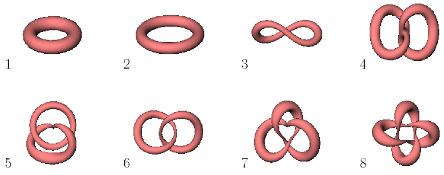
Figure 1: Position curves for the known lowest energy solitons with Hopf charges $1\leq Q\leq 8.$

$Q$	Type	$E$	$E/Q^{3/4}$
1	${\cal A}_{1,1}$	1.000	1.000
2	${\cal A}_{2,1}$	1.794	1.067
3	$\widetilde{\cal A}_{3,1}$	2.535	1.112
4	${\cal L}_{1,1}^{1,1}$	3.156	1.116
5	${\cal L}_{1,2}^{1,1}$	3.739	1.118
6	${\cal L}_{2,2}^{1,1}$	4.339	1.132
7	${\cal K}_{3,2}$	4.843	1.125
8	${\cal L}_{2,2}^{2,2}$	5.297	1.114

Table 1: Energies and types of the known minimal energy solitons with $1\leq Q\leq 8.$

Figure 2: The ratio of the energy $E$ to the conjectured bound $Q^{3/4}$ for the known minimal energy solitons with $1\leq Q\leq 8.$

In the Skyrme-Faddeev model the minimal energy soliton with $Q=4$ is axially symmetric and is of the type ${\cal A}_{2,2}$ [5]. A solution of this type has been constructed in the Nicole model using toroidal coordinates [10]. We have computed this solution, using initial conditions (3.3) with $(n,m)=(2,2),$ but found that, in constrast to the Skyrme-Faddeev model, this solution is unstable to perturbations that break the axial symmetry. Such a perturbation leads to the linked solution displayed in Figure 1.4, which is of the type ${\cal L}_{1,1}^{1,1}.$ We have also confirmed that the same solution is obtained by starting with the initial conditions (3.5) with $n=1.$ The energy of this solution can be found in Table 1.

Solitons with $Q=5,6,7,8$ have been constructed using a variety of initial conditions for each $Q$, including perturbed axial fields, links and knots. The resulting minimal energy solitons for each $Q$ are displayed in Figure 1 and their energies and types are listed in Table 1. For $Q=5,6$ the solitons are links and have the same type as in the Skyrme-Faddeev model. For $Q=7$ the soliton is a trefoil knot and again this agrees with the result of the Skyrme-Faddeev model. For $Q=8$ the soliton is a link of type ${\cal L}_{2,2}^{2,2}.$ In the Skyrme-Faddeev model the minimal energy soliton with $Q=8$ is also a link, but it has the different type ${\cal L}_{3,3}^{1,1}.$ In the Skyrme-Faddeev model initial conditions of the type ${\cal L}_{2,2}^{2,2}$ develop reconnections during the energy minimization process and this produces the minimal energy link ${\cal L}_{3,3}^{1,1}$ [6].

In the Skyrme-Faddeev model it has been shown [16] that a lower bound on the energy exists of the form $E\geq k\,Q^{\frac{3}{4}},$ where $k$ is a known constant. To date, a similar lower bound has not been proved for the Nicole model: see [10] for a discussion of the technical difficulties in adapting the proof in [16] to the Nicole model. A conjectured lower bound for the Nicole model is $E\geq Q^{\frac{3}{4}},$ where the constant has been set to unity, as this is the largest possible value consistent with the energy of the explicit $Q=1$ solution. In the final column of Table 1 we list the ratio of the energy to this conjectured bound and plot this ratio in Figure 2. It is clear that our numerical results are consistent with the conjectured bound. Furthermore, for $Q>2$ the excess above the bound appears to settle down to a value around $12\%,$ which suggests that the solutions we have found are good candidates for the global energy minima for these values of $Q.$

5 Conclusion

By introducing a volume-preserving flow we have been able to numerically investigate Hopf solitons and their stability in the Nicole model. It has been demonstrated that the known axially symmetric Hopf solitons are unstable for Hopf charges greater than two and new lower energy solutions have been computed that include links and knots. The formation of links and knots mirrors the situation in the Skyrme-Faddeev model, suggesting that this is likely to be a universal feature of Hopf solitons. However, for Hopf charges four and eight, links are formed in the Nicole model that are not of the same topological type as in the Skyrme-Faddeev model. As the Hopf charge increases there is an increased variety of possible link and knot types, so it seems likely that it becomes more common for the soliton types to disagree in the two theories.

A lower bound on the energy has been conjectured that is consistent with the numerical results we have obtained. A proof of this conjectured bound would signal another universal feature of Hopf solitons.

The Aratyn-Ferreira-Zimerman (AFZ) model [17] is another conformal field theory with Hopf soliton solutions. As in the Nicole model, the conformal symmetry allows the consistent use of a toroidal ansatz to reduce to an ordinary differential equation for a profile function [8]. In the AFZ model the profile function and associated energy can be obtained exactly in closed form [18] for all solutions of the type ${\cal A}_{n,m}.$ This is a consequence of an additional infinite-dimensional symmetry group acting on target space. It would be interesting to study the stability of these solutions and to investigate the existence of knotted and linked Hopf solitons in the AFZ model. There are additional complications in the AFZ model, related to the infinite-dimensional symmetry of the theory, as discussed in [19]. The approach of volume-preserving flow therefore needs some modification to be applicable to this model. This issue is currently under investigation.

References

- [1] L. D. Faddeev, Quantization of solitons, Princeton preprint IAS-75-QS70 (1975).
- [2] L. Faddeev and A. J. Niemi, Nature 387, 58 (1997).
- [3] J. Gladikowski and M. Hellmund, Phys. Rev. D56, 5194 (1997).
- [4] R. A. Battye and P. M. Sutcliffe, Phys. Rev. Lett. 81, 4798 (1998); Proc. R. Soc. Lond. A455, 4305 (1999).
- [5] J. Hietarinta and P. Salo, Phys. Lett. B451, 60 (1999); Phys. Rev. D62, 081701(R) (2000).
- [6] P. M. Sutcliffe, Proc. R. Soc. Lond. A463, 261 (2007).
- [7] D. A. Nicole, J. Phys. G4, 1363 (1978).
- [8] O. Babelon and L. A. Ferreira, JHEP 0211, 20 (2002).
- [9] B. M. A. G. Piette, B. J. Schroers and W. J. Zakrzewski, Z. Phys. C65, 165 (1995).
- [10] C. Adam, J. Sanchez-Guillen, R. A. Vazquez and A. Wereszczynski, J. Math. Phys. 47, 052302 (2006).
- [11] F. Lin and Y. Yang, Commun. Math. Phys. 249, 273 (2004).
- [12] M. Lüscher, Nucl. Phys. B200, 61 (1982).
- [13] R. A. Leese, M. Peyrard and W. J. Zakrzewski, Nonlinearity 3, 387 (1990).
- [14] R. S. Ward, Lett. Math. Phys. 35, 385 (1995).
- [15] M. Gillard and P. M. Sutcliffe, Proc. R. Soc. Lond. A465, 2911 (2009).
- [16] A. F. Vakulenko and L. V. Kapitanski, Dokl. Akad. Nauk USSR 246, 840 (1979).
- [17] H. Aratyn, L.A. Ferreira, A.H. Zimerman, Phys. Lett. B456, 162 (1999).
- [18] H. Aratyn, L.A. Ferreira, A.H. Zimerman, Phys. Rev. Lett. 83, 1723 (1999).
- [19] C. Adam, J. Sanchez-Guillen and A. Wereszczynski, J. Math. Phys. 48, 22305 (2007).