The Two-Dimensional Square-Lattice S=1/2 Antiferromagnet Cu(pz)₂(ClO₄)₂

Abstract

We present an experimental study of the two-dimensional S=1/2 square-lattice antiferromagnet Cu(pz)₂(ClO₄)₂ (pz denotes pyrazine - $\rm C_{4}H_{4}N_{2}$) using specific heat measurements, neutron diffraction and cold-neutron spectroscopy. The magnetic field dependence of the magnetic ordering temperature was determined from specific heat measurements for fields perpendicular and parallel to the square-lattice planes, showing identical field-temperature phase diagrams. This suggest that spin anisotropies in Cu(pz)₂(ClO₄)₂ are small. The ordered antiferromagnetic structure is a collinear arrangement with the magnetic moments along either the crystallographic b- or c-axis. The estimated ordered magnetic moment at zero field is $\rm m_{0}=0.47(5)\;\mathrm{\mu_{B}}$ and thus much smaller than the available single-ion magnetic moment. This is evidence for strong quantum fluctuations in the ordered magnetic phase of Cu(pz)₂(ClO₄)₂. Magnetic fields applied perpendicular to the square-lattice planes lead to an increase of the antiferromagnetically ordered moment to $\rm m_{0}=0.93(5)\;\mathrm{\mu_{B}}$ at $\rm\mu_{0}H=13.5\;\mathrm{T}$ - evidence that magnetic fields quench quantum fluctuations. Neutron spectroscopy reveals the presence of a gapped spin excitations at the antiferromagnetic zone center, and it can be explained with a slightly anisotropic nearest neighbor exchange coupling described by $\rm J_{1}^{xy}=1.563(13)\;\mathrm{meV}$ and $\rm J_{1}^{z}=0.9979(2)J_{1}^{xy}$.

I Introduction.

Low dimensional quantum magnets are of great fundamental interest. Unlike three-dimensional magnets, they support strong quantum fluctuations which can result in novel quantum excitations and novel ground states. Case in point is the antiferromagnetic S=1 chain whose ground state features hidden quantum order and is separated by a finite energy from excited states Haldane ; Buyers . In contrast, antiferromagnetic S=1/2 Heisenberg chains are gapless and feature fractionalized spin excitations as the hallmark of quantum criticality Tennant .

Increasing the dimensionality of a quantum magnet from one to two dimensions generally reduces effects of quantum fluctuations. The ground state of S=1/2 square lattice Heisenberg antiferromagnet (AF) adopts Néel long-range order at zero temperature. Nevertheless, strong quantum fluctuations arising from geometrical frustration may destroy long-range order in two dimensions.

Numerical studies of the two-dimensional (2D) S=1/2 Heisenberg AF on a square lattice using quantum Monte Carlo, exact diagonalization, coupled cluster as well as series expansion calculations reveal a quantum renormalization of the one-magnon energy in the entire Brillouin zone and the existence of a magnetic continuum at higher energies Singh ; Sandvik ; Zheng ; Ho ; igarashi ; singh . In recent years, quantum renormalization effects at zero field have been studied using neutron scattering in a number of good realizations of S=1/2 square-lattice Heisenberg AFs clarke2 ; ronnow ; Harris ; Christensen ; lumsden ; McMorrow . The addition of antiferromagnetic next-nearest neighbor (NNN) interactions destabilizes the antiferromagnetic ground state and increases quantum fluctuations: according to the $\rm J_{1}-J_{2}$ model Chandra ; Chandra2 ; Read ; Viana , where $\rm J_{1}$ and $\rm J_{2}$ are the nearest neighbor (NN) and the NNN exchange interactions, respectively, different ground states are stabilized as a function of $\rm J_{2}/J_{1}$. A possible spin-liquid phase appears to be the ground state for $\rm 0.38<J_{2}/J_{1}<0.6$ and collinear order was found for $\rm J_{2}/J_{1}>0.6$. Our previous study tsyrulin of Cu(pz)₂(ClO₄)₂ has shown that even a small $\rm J_{2}/J_{1}\simeq 0.02$ ratio enhances quantum fluctuations drastically, leading to a strong magnetic continuum at the antiferromagnetic zone boundary and the inversion of the zone boundary dispersion in magnetic fields.

Here we present an experimental investigation of the 2D organo-metallic AF Cu(pz)₂(ClO₄)₂, a good realization of the weakly frustrated $\rm J_{2}/J_{1}\simeq 0.02$ quantum AF on a square lattice with $\rm J_{1}\sim 1.56\;\mathrm{meV}$. Due to the small energy scale of the dominant exchange interaction, magnetic fields available for macroscopic measurements and neutron scattering allow the experimental investigation of this interesting model system for magnetic fields up to about one third of the saturation field strength. We combine specific heat, neutron diffraction and neutron spectroscopy to determine the spin Hamiltonian and the key magnetic properties of this model material. Specific heat measurements show that the magnetic properties are nearly identical for fields applied parallel and perpendicular to the square-lattice plane. This shows that spin anisotropies are small in contrast to spatial anisotropies, and that it is sufficient to perform microscopic measurement for just one field direction. Our microscopic neutron measurements, on the other hand, provide information on the spin Hamiltonian that explain the nearly identical HT phase diagrams for the two field directions. Specific heat and neutron measurements of Cu(pz)₂(ClO₄)₂ thus ideally complement each other.

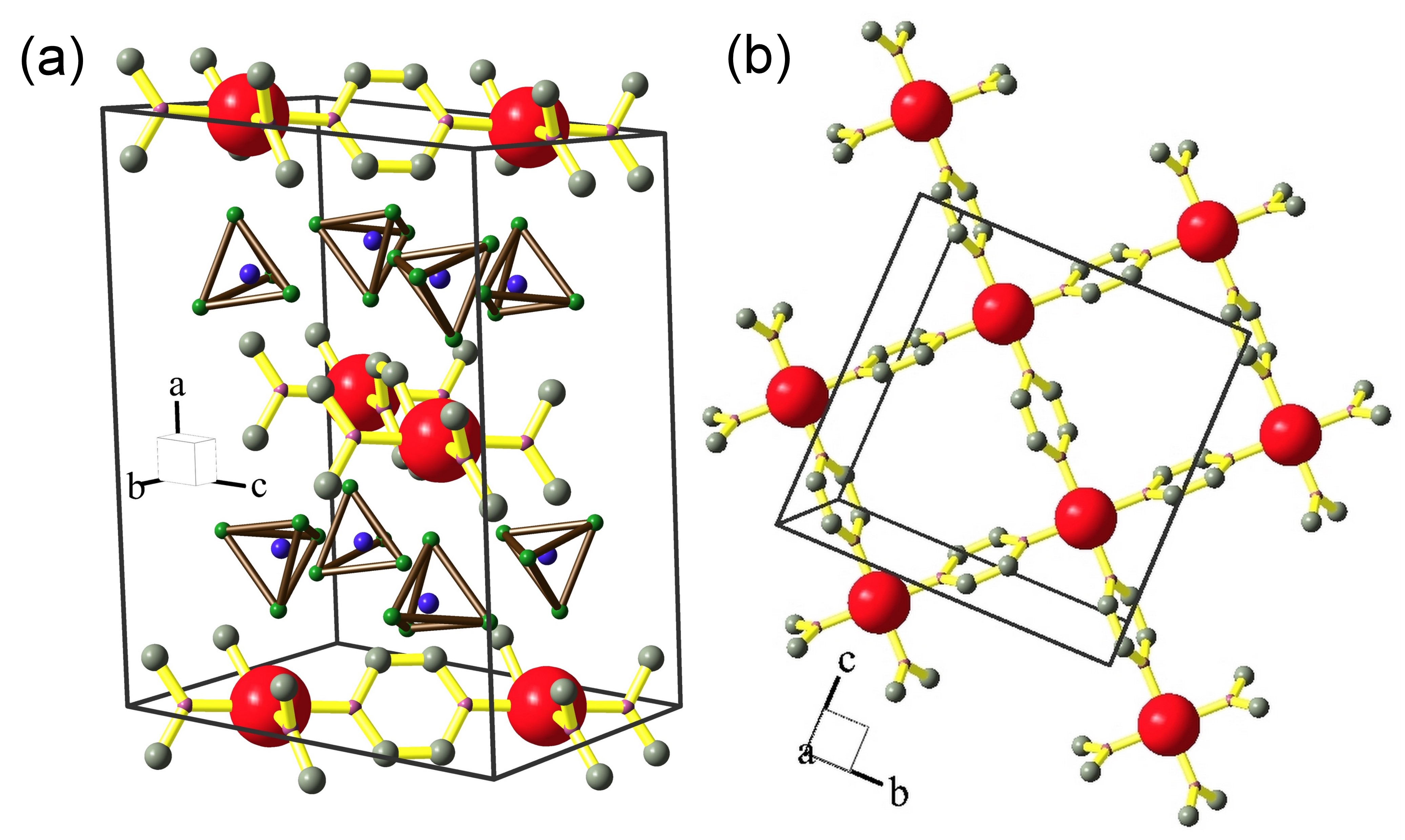
Figure 1: (Color online) (a) Three-dimensional view of the crystal structure of Cu(pz)₂(ClO₄)₂. The $\rm Cu^{2+}$ ions are shown as big spheres. The $\rm ClO_{4}$ tetrahedra are located between the copper layers and pyrazine molecules link ${\rm Cu^{2+}}$ in $bc$-plane. The D atoms are not shown for simplicity. (b) The projection of the crystal structure on the $bc$-plane shows the ${\rm Cu^{2+}}$ square-lattice structure. The square lattice are shifted by (0,0.5,0) from one layer to the next.

Deuterated copper pyrazine perchlorate Cu(pz)₂(ClO₄)₂ crystallizes in a monoclinic crystal structure described by space group C2/c, with lattice parameters $\rm a=14.045(5){\AA}$, $\rm b=9.759(3){\AA}$, $\rm c=9.800(3){\AA}$ and $\rm\beta=96.491(4)^{\circ}$ Wo . The crystal structure is shown in Fig. 1. The ${\rm Cu^{2+}}$ ions occupy 4e Wyckoff positions and pyrazine ligands link magnetic $\rm Cu^{2+}$ ions into square-lattice planes lying in the crystallographic $bc$-plane. The ${\rm Cu^{2+}}$-${\rm Cu^{2+}}$ NN distances in the $bc$-plane are identical and equal to 6.92$\rm{\AA}$ Wo . The two fold rotation axis (0, y, 1/2) and the mirror plane parallel to the $ac$-plane ensure that all NN exchange interactions between $\rm Cu^{2+}$ are identical. Tetrahedra of ClO₄ located between the planes (Fig. 1a) provide good spatial isolation of $\rm Cu^{2+}$ ions and substantially decrease the interlayer interactions. Thus, perfect square-lattices of copper ions with a superexchange path mediated by pyrazine molecules are formed in the $bc$-plane (Fig. 1b).

The magnetic susceptibility shows good agreement with that of the 2D S=1/2 Heisenberg AF with an exchange interaction strength of $\rm J_{1}=1.53(3)\;\mathrm{meV}$. Small interlayer interactions result in a long range antiferromagnetic order below $\rm T_{N}=4.21(1)\;\mathrm{K}$. The ratio of interlayer exchange, $\rm J_{\perp}$, to the dominant intralayer exchange strength, $\rm J_{1}$, was estimated as $\rm J_{\perp}/J_{1}=8.8\cdot 10^{-4}$  Wo ; Lancaster ; Xiao .

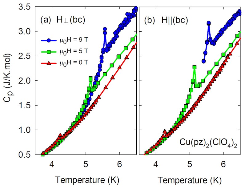
Figure 2: (Color online) Specific heat of Cu(pz)₂(ClO₄)₂ as a function of temperature for different magnetic field strengths. The measurements for magnetic fields parallel and perpendicular to the $bc$-plane are shown in (a) and (b), respectively. For convenience the graphs are shown as lines connecting the data points and without error bars.

II Experimental details.

In order to obtain the field-temperature (HT) phase diagram of Cu(pz)₂(ClO₄)₂ we measured the specific heat as a function of temperature for different magnetic field strengths using the Physical Property Measurement System by Quantum Design. A single crystal of deuterated Cu(pz)₂(ClO₄)₂ with mass $\rm m=13\;\mathrm{mg}$ was fixed on a sapphire chip calorimeter with Apiezon-N grease. The measurements were done using the relaxation technique which consists of the application of a heat pulse to a sample and the subsequent tracking the induced temperature change. The specific heat was obtained in the range from $\rm T=2\;\mathrm{K}$ to $\rm T=30\;\mathrm{K}$ in magnetic fields of up to $\rm\mu_{0}H=9\;\mathrm{T}$ applied parallel and perpendicular to the copper square-lattice planes. The measurements were done with the steps of $\rm\Delta T_{1}=0.05\;\mathrm{K}$, $\rm\Delta T_{2}=0.2\;\mathrm{K}$ and $\rm\Delta T_{3}=1\;\mathrm{K}$ in the temperature ranges $\rm T_{1}=2-6\;\mathrm{K}$, $\rm T_{2}=6-8\;\mathrm{K}$ and $\rm T_{3}=8-30\;\mathrm{K}$, respectively. Care was taken to apply a small heat pulse of $\rm 0.1\%$ of the temperature step $\rm\Delta T$ and each measurement was repeated three times to increase accuracy. Specific heat of Apiezon-N grease without Cu(pz)₂(ClO₄)₂ crystal was measured in the entire temperature range separately and subtracted as a background from the total specific heat of the sample and grease.

Figure 3: (Color online) Neutron scattering peak intensity of $\textbf{Q}=(0,1,0)$ as a function of temperature and magnetic field, applied perpendicular to the square-lattice planes. The results obtained by specific heat measurements in magnetic field applied parallel and perpendicular to the Cu planes are shown by squares and circles, respectively. The neutron data, measured for magnetic fields perpendicular to the copper planes, are shown by triangles.

The HT phase diagram and the ordered magnetic structure were studied by neutron diffraction using cold-neutron three-axis spectrometer RITA2 at the Paul Scherrer Institute, Villigen, Switzerland. A crystal with dimensions $7\times 7\times 1.5\;\mathrm{mm}$ and mass of $\rm m=85\;\mathrm{mg}$ was wrapped into aluminum foil, fixed with wires on a sample holder and aligned with its reciprocal [0, k, l] plane in the horizontal scattering plane of the neutron spectrometer. Data were collected at $\rm T=2.3\;\mathrm{K}$ and $\rm T=10\;\mathrm{K}$ in magnetic fields up to $\rm\mu_{0}H=13.5\;\mathrm{T}$ applied nearly perpendicular to the [0, k, l] plane using an Oxford cryomagnet. Measurements were performed with the pyrolytic graphite (PG) (002) Bragg reflection as a monochromator. A cooled Be filter was installed before the analyzer to suppress higher order neutron contamination for the final energy $\rm E_{f}=5\;\mathrm{meV}$. We also used an experimental setup without Be filter, which allowed to use the second order neutrons from the monochromator with $\rm E_{i}=20\;\mathrm{meV}$, thus allowing to access to reflections at high wave-vector transfers.

The spin dynamics in the antiferromagnetically ordered phase was measured using the cold-neutron three-axis spectrometer PANDA at FRM-2, Garching, Germany. Two single crystals with a total mass of $\rm m=1\;\mathrm{g}$ were wrapped into aluminum foil, fixed on a sample holder with wires and co-aligned in an array with a final mosaic spread of $1^{\circ}$. Reciprocal [0, k, l] plane of the sample was aligned with the horizontal scattering plane of the neutron spectrometer. These measurements were performed in zero magnetic field and at temperature $\rm T=1.42\;\mathrm{K}$ using a $\rm{}^{4}He$ cryostat generally referred to as an Orange cryostat. The final energy was either set to $\rm E_{f}=4.66\;\mathrm{meV}$ or $\rm E_{f}=2.81\;\mathrm{meV}$ using a PG(002) analyzer. Data were collected using a PG(002) monochromator and cooled Be filter installed before the analyzer.

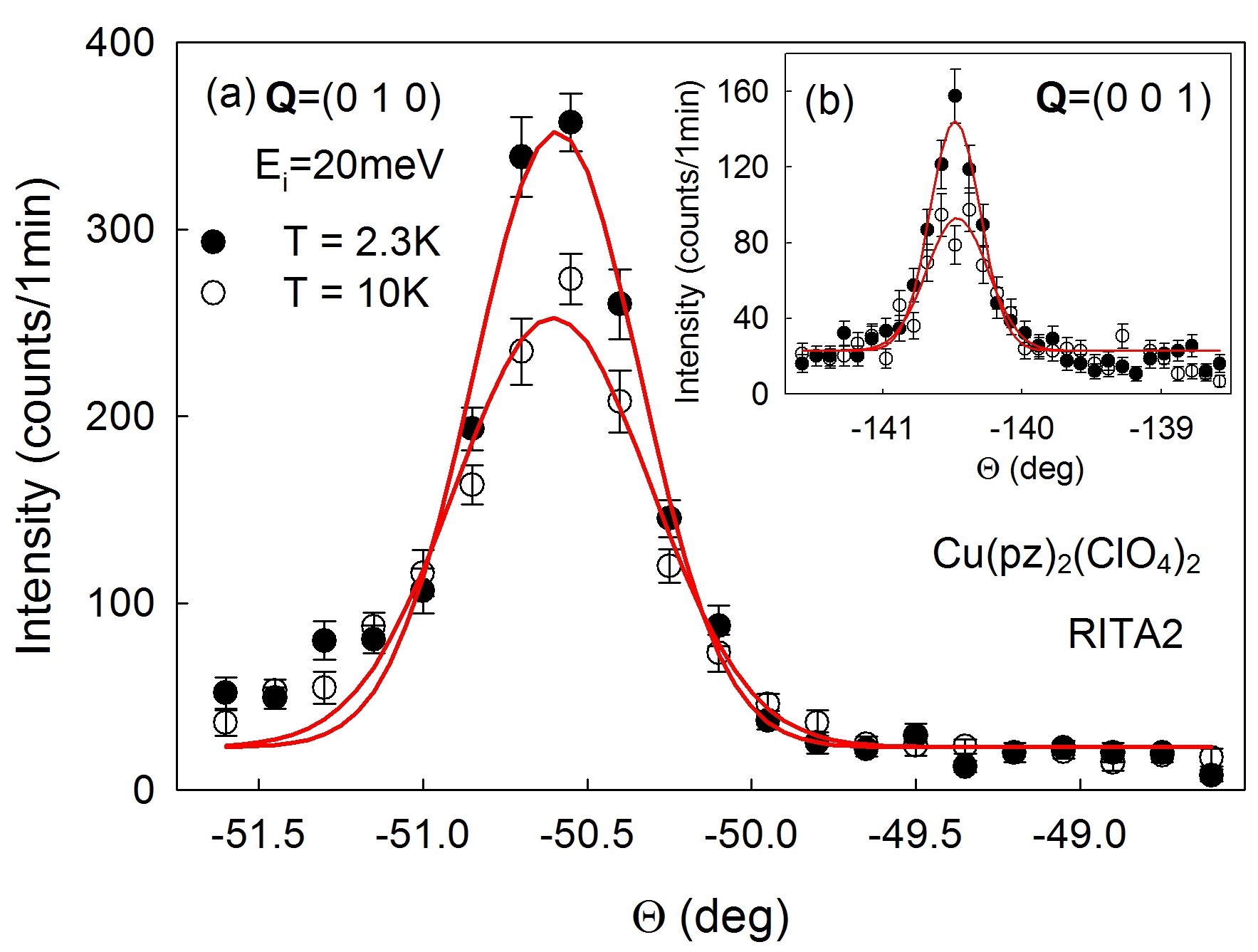
Figure 4: (Color online) (a) Neutron scattering intensity at $\textbf{Q}=(0,1,0)$ measured at $T=2.3\;\mathrm{K}$ and at $T=10\;\mathrm{K}$ as a function of a rotation of the sample around the vertical axis described by angle $\Theta$. The inset (b) shows the neutron scattering observed at $\textbf{Q}=(0,0,1)$ at the same temperature.

III Results.

III.1 Specific heat measurements.

The temperature dependence of the specific heat of Cu(pz)₂(ClO₄)₂ is shown in Fig. 2 for different magnetic fields applied perpendicular and parallel to the copper square-lattice plane. At all fields, the temperature dependence of the specific heat reveals a well defined cusp-like peak, indicating a second order phase transition towards 3D long-range magnetic order. Previous zero-field studies of Cu(pz)₂(ClO₄)₂ did not show an anomaly in the specific heat Lancaster . Most likely, the high accuracy of our measurements played a crucial role in detecting the zero-field anomaly in the specific-heat curve. The small size of the ordering anomaly is a consequence of the low dimensionality of the magnetism and an ordered magnetic moment that, due to quantum fluctuations, is considerably smaller than the free-ion value. The HT phase diagram assembled from the specific heat measurements is shown in Fig. 3. The measurements show that the Néel temperature increases with increasing magnetic field, from $\rm T_{N}=4.24(4)\;\mathrm{K}$ at zero field to $\rm T_{N}=5.59(3)\;\mathrm{K}$ at $\rm\mu_{0}H=9\;\mathrm{T}$.

We also observe an increase of the specific heat with increasing magnetic field in the paramagnetic phase just above the 3D ordering temperature. We propose that the field dependence of the specific heat data is a consequence of field-induced anisotropy in the 2D AF. In zero field, a pure 2D Heisenberg AF orders at zero temperature, but quantum Monte Carlo simulations Cuccoli03 have shown that application of an external field induces an Heisenberg-XY crossover and leads to a finite temperature Berezinskii-Kosterlitz-Thouless transition $T_{\mathrm{BKT}}$ BKT1 ; BKT2 . One consequence of this crossover is the increase of $T_{\mathrm{BKT}}$ with external field for up to $H<H_{\mathrm{SAT}}/4$ and then a gradual decrease of the transition temperature with increased fields. While the zero-field 3D transition $T_{N}$ in Cu(pz)₂(ClO₄)₂ is driven by the combination of 3D interaction and intrinsic XY anisotropy, the increase of $T_{N}$ as a function of field may thus be driven by an increase of the effective anisotropy and the associated increase of $T_{\mathrm{BKT}}$. Similarly, we propose that the increase of the specific heat above the 3D ordering temperature is caused by the field-induced XY anisotropy: In the 2D antiferromagnet on a square lattice, 2D topological spin-vortices appear above the Berezinskii-Kosterliz-Trousers (BKT) transition as the preferable thermodynamic configuration. In applied magnetic field the vortices unbind above the BKT transition, leading to the increase of the specific heat above the ordering temperature. The anisotropy crossover thus affects the specific heat in a manner similar to the observed behavior Cuccoli03 .

Remarkably, the HT phase diagrams are identical for fields parallel and perpendicular to the square-lattice planes. This suggests that the dominant exchange interactions between nearest copper spins $J_{1}$ in $bc$-plane are close to the isotropic limit in spin space. This should not be confused with the strong spatial two-dimensionality of Cu(pz)₂(ClO₄)₂.

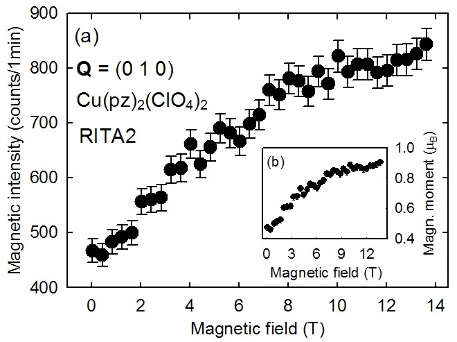
Figure 5: The magnetic peak intensity of neutron scattering at $\textbf{Q}=(0,1,0)$ as function of magnetic field measured at $\rm T=2.3\;\mathrm{K}$. The non-magnetic scattering was estimated from measurements at $\rm T=10\;\mathrm{K}$ and subtracted from the overall peak intensity. The inset shows the ordered antiferromagnetic moment as a function of field.

III.2 Magnetic order parameter.

To determine the ordered magnetic structure of Cu(pz)₂(ClO₄)₂, several magnetic Bragg reflections were measured by neutron diffraction. Fig. 4 shows two magnetic peaks measured above and below the transition temperature at $\textbf{Q}=(0,1,0)$ and $\textbf{Q}=(0,0,1)$ using a final energy $\rm E_{f}=20\;\mathrm{meV}$. This data directly demonstrates the presence of magnetic order below $\rm T_{N}$. The magnetic Bragg peak widths are limited by the instrumental resolution, confirming that the magnetic order is long-range. The field dependence of the magnetic scattering at $\textbf{Q}=(0,1,0)$ measured using final energy $\rm E_{f}=5\;\mathrm{meV}$ reveals an increase of magnetic intensity as a function of field from zero to $\rm\mu_{0}H=13.5\;\mathrm{T}$ as is shown in Fig. 5. The magnetic scattering was determined by subtracting the non-magnetic background determined at T = 10K. The increase of magnetic diffraction intensity with field is most probably related to a quenching of quantum fluctuations by the magnetic field, that simultaneously also leads to the observed increase of the transition temperature $\rm T_{N}$. This result is in a good agreement with the specific heat data indicating enhanced XY anisotropy in the applied magnetic field. The intensity measured at $\textbf{Q}=(0,1,0)$ at $\rm T=10\;\mathrm{K}$ as the function of applied field did not reveal any magnetic scattering, showing that magnetic fields do not lead to field-induced antiferromagnetic order in the paramagnetic phase.

The critical magnetic behavior was studied by measuring the peak intensity of the neutron scattering at the antiferromagnetic wave vector $\textbf{Q}=(0,1,0)$ and $\textbf{Q}=(0,3,0)$ as function of temperature in magnetic field up to $\rm\mu_{0}H=13.5\;\mathrm{T}$. Typical scans are shown in Fig. 6. The solid line display that the increase of the antiferromagnetic intensity in the ordered phase close to $\rm T_{N}$ is evidently steeper for high fields. The HT phase diagram compiled from the temperature scans is shown in Fig. 3 and it confirms the phase diagram obtained from specific heat measurements.

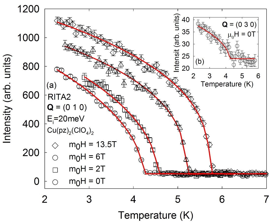
Figure 6: (Color online) (a) The temperature dependence of the neutron scattering peak intensity measured at the antiferromagnetic point $\textbf{Q}=$(0, 1, 0). The data collected at $\rm\mu_{0}H=0\;\mathrm{T}$, $\rm\mu_{0}H=2\;\mathrm{T}$ $\rm\mu_{0}H=6\;\mathrm{T}$ and $\rm\mu_{0}H=13.5\;\mathrm{T}$ are shown by circles, squares, triangles and diamonds, respectively. The red lines are guides to the eye. The inset (b) represents the peak intensity at $\textbf{Q}=(0,3,0)$ as the function of temperature obtained at zero field. $\rm T_{N}$ was found to be the same as for $\textbf{Q}=(0,1,0)$.

III.3 Ordered magnetic structure.

The symmetry of the ordered magnetic phase was studied by neutron diffraction. Group theory was used to restrict the search only to magnetic structures that are allowed by symmetry. The magnetic Bragg peaks at $\textbf{Q}=(0,1,0)$ and $\textbf{Q}=(0,3,0)$ indicate that the magnetic structure breaks the C-centering of the chemical lattice and that Cu(pz)₂(ClO₄)₂ adopts an antiferromagnetic structure for $\rm T<T_{N}$. Symmetry analysis revealed six basis vectors which belong to four irreducible representations and are listed in Tab. 3 (for details see Appendix A).

The analysis is complicated by the fact that the single-crystal probably consists of two domains with interchanged $b$- and $c$-axis, which are nearly identical in length. A twinning of the single-crystal in this manner is indicated by the observation of both the $\rm\textbf{Q}=(0,2,3)$ and $\textbf{Q}=(0,3,2)$ nuclear Bragg peaks with similar intensity, although $\textbf{Q}=(0,3,2)$ is not allowed for a C-centered lattice.

The experimental data are consistent with both $\Gamma_{2}$ and $\Gamma_{4}$ irreducible representations listed in Tab. 2 and with two basis vectors $\overrightarrow{\phi}_{2}$ and $\overrightarrow{\phi}_{6}$. It is not possible to distinguish between these two solutions because $\overrightarrow{\phi}_{2}$ of the $bc$ crystallographic domain is identical to $\overrightarrow{\phi}_{6}$ of the $cb$ crystallographic domain, and the fits were made assuming a equal population of $bc$ and $cb$ crystallographic domains. The ordered magnetic structure of Cu(pz)₂(ClO₄)₂ can have magnetic moments aligned antiferromagnetically either along crystallographic $b$- or $c$-axis as is shown in Fig. 7(a) and Fig. 7(b), respectively. Due to a small number of observed magnetic reflections and the crystallographic twinning, our experiment cannot distinguish between these two magnetic structures. The collinear spin arrangement in $bc$-plane is consistent with the absence of the Dzyaloshinsky-Moriya interactions between NN. The spatial arrangement of the ordered magnetic moments in adjacent square-lattice layers is ferro- and antiferromagnetic along $ab$- and $ac$-diagonal, respectively. This is consistent with the chemical structure of Cu(pz)₂(ClO₄)₂, where the interlayer interaction pathway along $ac$-diagonal is shorter than the path along $ab$.

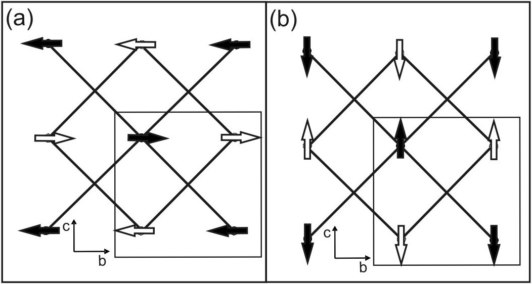
Figure 7: Two possible magnetic structures of Cu(pz)₂(ClO₄)₂ belonging to the second and the fourth irreducible representations (see Tab. 2), are shown in (a) and (b), respectively. Two adjacent square-lattice $\rm Cu^{2+}$ layers, separated by a (0.5,0.5,0) lattice unit translation, are depicted by open and filled arrows. $\rm Cu^{2+}-Cu^{2+}$ interlayer interaction pathway along $ac$ diagonal corresponds to the vertical distance between filled and open symbols in (a) and (b).

The value of the ordered magnetic moment was obtained from a minimization of $\rm\delta=|R_{calc}-R_{exp}|$, where $\rm R_{exp}$ is the measured ratio of the magnetic Bragg peak intensity to the nuclear Bragg peak intensity, $\rm R_{calc}=\rm|F(\textbf{Q})_{magn}|^{2}/|F(\textbf{Q})_{nucl}|^{2}$, $\rm F(\textbf{Q})_{magn}$ and $\rm F(\textbf{Q})_{nucl}$ are the magnetic and nuclear structure factors, respectively. The fit was performed for two magnetic peaks observed at $\textbf{Q}=(0,1,0)$ and $\textbf{Q}=(0,3,0)$ and two nuclear peaks measured at $\textbf{Q}=(0,2,4)$ and $\textbf{Q}=(0,0,6)$. The obtained value of the ordered magnetic moment in zero field is $\rm m_{0}=0.47(5)\;\mathrm{\mu_{B}}$. The comparison of $\rm R_{calc}$ and $\rm R_{exp}$ for

	$\frac{|F(0,1,0)|^{2}}{|F(0,2,4)|^{2}}$	$\frac{|F(0,1,0)|^{2}}{|F(0,0,6)|^{2}}$	$\frac{|F(0,3,0)|^{2}}{|F(0,2,4)|^{2}}$	$\frac{|F(0,3,0)|^{2}}{|F(0,0,6)|^{2}}$
$\rm R_{exp}\times 10^{-4}$	3.72(7)	5.13(12)	1.89(18)	2.60(25)
$\rm R_{calc}\times 10^{-4}$	4.35	4.57	2.16	2.26

Table 1: The measured and the calculated ratios of squared magnetic to nuclear structure factors for different Bragg peaks. The calculated values were obtained from a minimization of $\rm\delta=|R_{calc}-R_{exp}|$ and correspond to the ordered magnetic moment $\rm m_{0}=0.47\mu_{B}$.

two magnetic and two nuclear Bragg peaks is presented in the Tab. 1. The calculated value of the ordered magnetic moment is smaller than the free-ion magnetic moment, indicating the presence of strong quantum fluctuations in the magnetic ground state of Cu(pz)₂(ClO₄)₂. The inset (b) in Fig. 5 displays the increase of the ordered antiferromagnetic moment from $\rm m_{0}=0.47(5)\mu_{B}$ in zero field to $\rm m_{0}=0.93(5)\;\mathrm{\mu_{B}}$ in $\rm\mu_{0}H=13.5\;\mathrm{T}$. This is direct evidence for the suppression of quantum fluctuations by the applied magnetic field due to induced XY anisotropy as suggested by our specific heat measurements.

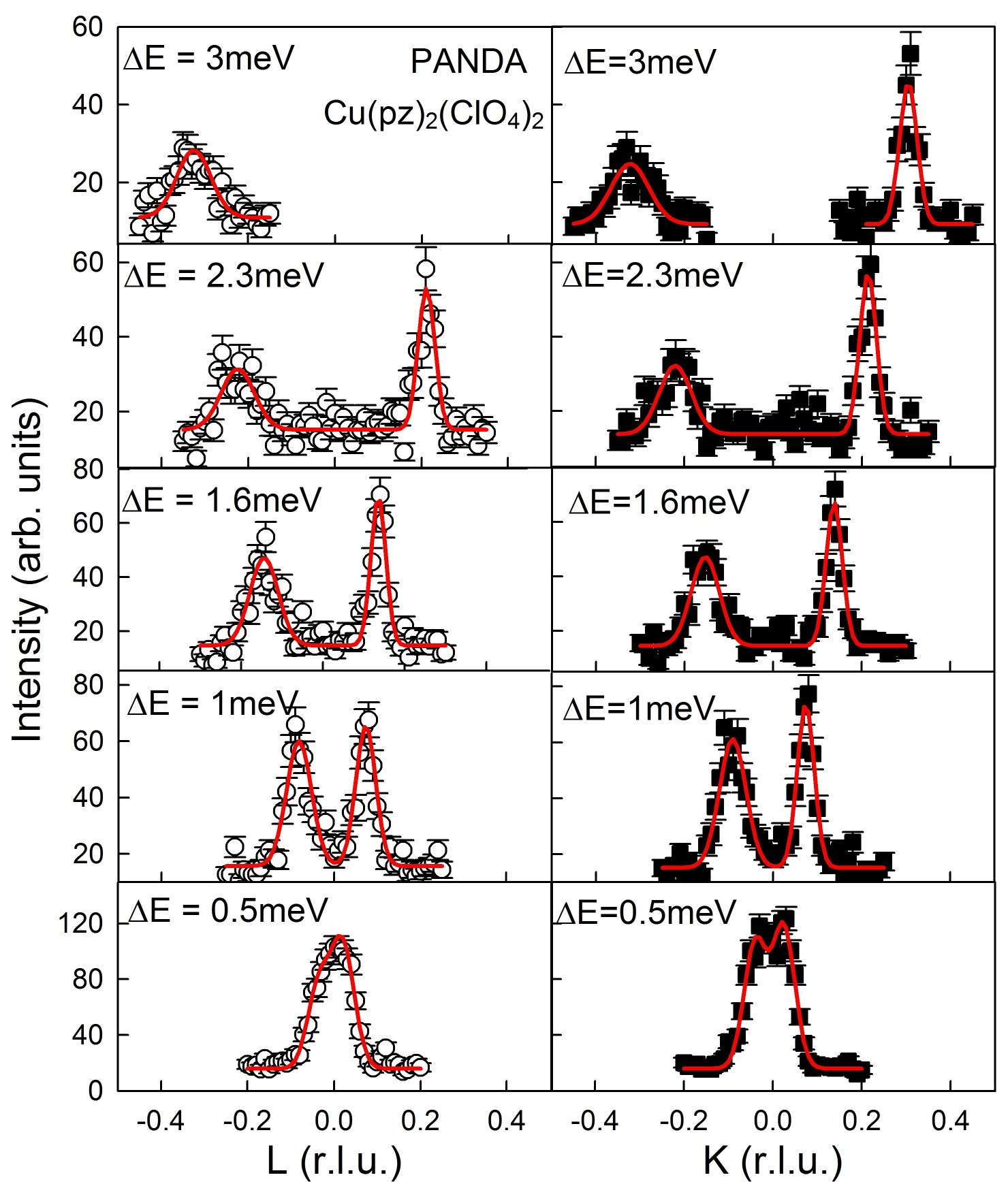
Figure 8: (Color online) A series of constant energy scans performed along the [0, k, 1] and [0, -1, l] directions at different energy transfers $\rm\Delta E$ in zero magnetic field and at $\rm T=1.42\;\mathrm{K}$. Please note the changing scale of the vertical axis for the different scans. The solid lines correspond to a convolution of two Gaussians with the resolution function.

III.4 Spin dynamics.

The wave-vector dependence of the magnetic excitations has been measured using neutron spectroscopy. Constant energy scans were performed near the antiferromagnetic zone centers $\textbf{Q}=(0,0,1)$ and $\textbf{Q}=(0,-1,0)$ for energy transfer $\rm\Delta E$ in the range from $\rm\Delta E=0.5\;\mathrm{meV}$ to $\rm\Delta E=3\;\mathrm{meV}$ and are shown in Fig. 8. The observed magnetic peaks are resolution limited, indicating that these magnetic excitations are long-lived magnons associated with a long-range ordered magnetic structure.

Constant wave-vector scans were performed at the antiferromagnetic zone centers in the energy transfer range from $\rm\Delta E=0\;\mathrm{meV}$ to $\rm\Delta E=0.7\;\mathrm{meV}$ (Fig. 9a, b). These scans reveal a magnetic mode which is gapped and has a finite energy $\rm E_{zc}=0.201(8)\;\mathrm{meV}$ at the antiferromagnetic zone center. The energy gap at the antiferromagnetic zone center is attributed to the presence of a small XY anisotropy in the nearest-neighbor two-ion exchange interactions, because a single-ion anisotropy of type $\rm\textbf{D}(\textbf{S}^{z})^{2}$ is not allowed for S=1/2.

Constant wave-vector scans away from the antiferromagnetic zone center carried out at higher energies are shown in Fig. 9(c). The energies of the magnetic excitation at the symmetrically identical antiferromagnetic zone boundary points $\rm\textbf{Q}_{zb1}=(0,0.5,1)$ and $\rm\textbf{Q}_{zb2}=(0,-0.5,1)$ are equal to $\rm E_{zb1}=3.629(6)\;\mathrm{meV}$ and $\rm E_{zb2}=3.599(13)\;\mathrm{meV}$, respectively. The peaks observed in the constant wave-vector scans at $\rm\textbf{Q}_{zb1}$ and $\rm\textbf{Q}_{zb2}$ are resolution limited. This experimental fact together with the identity of the values $\rm E_{zb1}$ and $\rm E_{zb2}$ confirms the NN interactions in $bc$-plane are identical along the square-lattice directions. In case of different strengths for the NN interactions in $bc$-plane a broadening of the peaks at $\rm\textbf{Q}_{zb1}$ and $\rm\textbf{Q}_{zb2}$ would be observed. From our previous study tsyrulin we know that there is also a small NNN interaction equal to $2\%$ of the NN exchange interaction. Therefore the observed one-magnon mode was compared to the following model 2D Hamiltonian:

$$\rm\hat{H}=\sum_{\langle i,j\rangle}\{J_{1}^{z}\textbf{S}_{i}^{z}\cdot\textbf{S}_{j}^{z}+J_{1}^{xy}(\textbf{S}_{i}^{x}\cdot\textbf{S}_{j}^{x}+\textbf{S}_{i}^{y}\cdot\textbf{S}_{j}^{y})\}+J_{2}\sum_{\langle i,k\rangle}\textbf{S}_{i}\cdot\textbf{S}_{k},$$ (1)

where $\rm\langle i,j\rangle$ indicates the sum over NN in the $bc$-plane, $\rm\langle i,k\rangle$ - the sum over NNN in the $bc$-plane, $\rm J_{1}^{z}$, $\rm J_{1}^{xy}$ and $\rm J_{2}$ are $z$-, $xy$-components of the NN interaction and the NNN exchange, respectively.

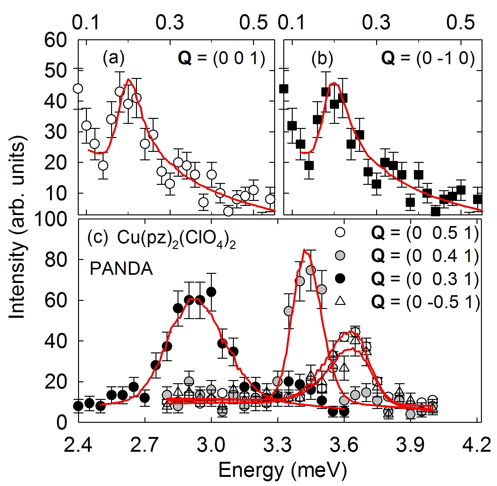
Figure 9: (Color online) The constant Q-scans collected at small energy transfer show the energy of a gapped spin-wave at the antiferromagnetic zone center performed at $\textbf{Q}=(0,0,1)$ and at $\textbf{Q}=(0,-1,0)$ are presented in (a) and (b), respectively. (c) Constant Q-scans performed close to the antiferromagnetic zone boundary at high energy transfer show the dispersion of the spin-wave. The measurements were performed in zero magnetic field and at $\rm T=1.42\;\mathrm{K}$. The solid lines represent the convolution of a Gaussian with the resolution function.

The linear spin wave theory (for details see Appendix B) yields two spin-wave modes with the dispersion $\rm\hbar\omega_{q}=\sqrt{A_{q}^{2}-B_{q}^{2}}$, where $\rm A_{q}=4SJ_{1}^{xy}+S(J_{1}^{xy}-J_{1}^{z})(\cos(\textbf{qb})+\cos(\textbf{qc}))-4SJ_{2}+4SJ_{2}\cos(\textbf{qb})\cdot\cos(\textbf{qc}))$ and $\rm B_{q}=S(J_{1}^{xy}+J_{1}^{z})(\cos(\textbf{qb})+\cos(\textbf{qc}))$. This implies that the exchange anisotropy mostly affects the magnon energy close to the antiferromagnetic zone center, while the zone boundary energy remains nearly unaffected by the exchange anisotropy. In the 2D S=1/2 AF, the energy of a classical (large-S) spin-wave mode is renormalized due to quantum fluctuations with the best theoretically predicted renormalization factor $\rm Z_{c}=1.18$ igarashi ; singh . Therefore the energy at the antiferromagnetic zone boundary is equal to $\rm E_{zb}=2Z_{c}J_{1}^{z}-J_{2R}$, where $\rm J_{2R}$ is the renormalized NNN interaction. The calculated $xy$-component of NN and NNN exchange interactions are equal to $\rm J_{1}^{xy}=1.563(13)\;\mathrm{meV}$ and $\rm J_{2}\simeq 0.02J_{1}^{xy}$, respectively. According to the linear spin wave theory $\rm E_{zc}^{2}=8J_{1}^{xy}(J_{1}^{xy}-J_{1}^{z})$ and thus $\rm J_{1}^{z}=0.9979(2)J_{1}^{xy}$.

The values of the $xy$- and $z$-components of the NN interaction obtained from our neutron measurements are in a good agreement with the result of magnetic susceptibility measurements Xiao , which yielded $\rm J_{1}^{xy}=1.507(26)\;\mathrm{meV}$ and $\rm J_{1}^{z}=0.9954J_{1}^{xy}$. The small XY anisotropy indicates that the dominant exchange interaction between nearest copper ions in $bc$-plane in Cu(pz)₂(ClO₄)₂, while spatially very anisotropic, is close to the isotropic limit in spin space, explaining the strong similarity of the HT phase diagrams measured in magnetic fields applied parallel and perpendicular to copper square-lattice (Fig. 3).

The inelastic-scattering data were fitted with the Gaussian instrumental resolution function convoluted numerically with the model Hamiltonian (1). The result of the fits is shown by the red lines in Fig. 8 and Fig. 9, and provides a good description of the observed spin waves. The color plot of the neutron scattering intensity, which is shown in Fig. 10, summarizes the observed magnetic excitations in both crystallographic directions. The black lines display the result of the linear spin wave theory, showing that the observed dispersive excitation is well characterized by the Hamiltonian (1).

The measured spin wave dispersion is similar to that observed in another 2D square-lattice antiferromagnetic material, namely copper deuteroformate tetradeuterate (CFTD), where the exchange interaction strength is equal to $\rm J=6.3(3)\;\mathrm{meV}$ and the energy gap of $\rm E=0.38(2)meV$ is present at the antiferromagnetic zone center. However, the energy gap in CFTD is induced by the presence of small antisymmetric Dzyaloshinsky-Moriya interaction $\rm\textbf{D}=0.0051(5)\;\mathrm{meV}$ between NN clarke2 ; ronnow . Another example with comparable properties is $\rm{K_{2}V_{3}O_{8}}$ with 2D NN exchange strength $\rm J=1.08(3)\;\mathrm{meV}$ and small energy gap at antiferromagnetic point equal to $\rm E=0.072(9)\;\mathrm{meV}$ lumsden , which is described by Dzyaloshinsky-Moriya and easy-axis anisotropies Chernyshev . In contrast, Dzyaloshinsky-Moriya interactions between NN in Cu(pz)₂(ClO₄)₂ are forbidden by symmetry and the energy gap at the antiferromagnetic zone center is generated by small XY anisotropy.

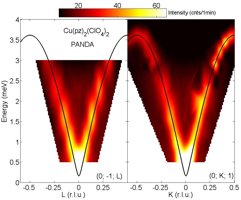
Figure 10: (Color online) Color plot of the scattering intensity, showing the dispersion along the $\textbf{Q}=(0,-1,l)$ and $\textbf{Q}=(0,k,1)$ directions measured at zero field, presented in the left and right panels, respectively. The color plot was obtained by merging a total of five and thirteen constant wave-vector scans, respectively. The solid line represents the dispersion computed from linear spin wave theory using $\rm J_{1}^{xy}=1.563\;\mathrm{meV}$, $\rm J_{1}^{z}=0.9979J_{1}^{xy}$ and NNN exchange equal to $\rm J_{2}=0.02J_{1}^{xy}$ as described in the text.

We also studied the spin-wave dynamics along the antiferromagnetic zone boundary by performing constant wave-vector scans along the $\textbf{Q}=(0,0.5,l)$ direction from $l=1$ to $l=2$. Typical data are shown in Fig. 11(a-c) and the observed zone boundary dispersion is shown in Fig. 11(d). The onset of the scattering at $\textbf{Q}=(0,0.5,1.5)$ is reduced by 10.7(4)% in energy compared to $\textbf{Q}=(0,0.5,1)$, confirming our recent independent measurement tsyrulin . The decrease of the resonant mode energy at $\textbf{Q}=(0,0.5,1.5)$ results from a resonating valence bond quantum fluctuations between NN spins Sandvik ; McMorrow . The observed dispersion at the zone boundary is slightly larger than expected from series expansion calculations and Quantum Monte Carlo simulations for 2D Heisenberg square-lattice AF with NN interactions Sandvik ; Zheng and can be explained by the presence of a small antiferromagnetic NNN interaction.

In order to subtract a nonmagnetic contribution from the background in the energy scan at $\textbf{Q}=(0,0.5,1.5)$ we performed measurements with the sample turned away from magnetic scattering. The background-subtracted data are shown in Fig. 11(a). The width of the scattering peak as a function of energy at $\textbf{Q}=(0,0.5,1.5)$ is clearly broader than the instrumental resolution. This implies the existence of a magnetic continuum scattering in this region of the antiferromagnetic zone boundary. The magnetic continuum with the present PANDA measurements is consistent with our previous investigation of Cu(pz)₂(ClO₄)₂ tsyrulin . This non-trivial magnetic continuum and the dispersion at the zone-boundary result from quantum fluctuations in Cu(pz)₂(ClO₄)₂ which are enhanced by a small antiferromagnetic NNN interaction.

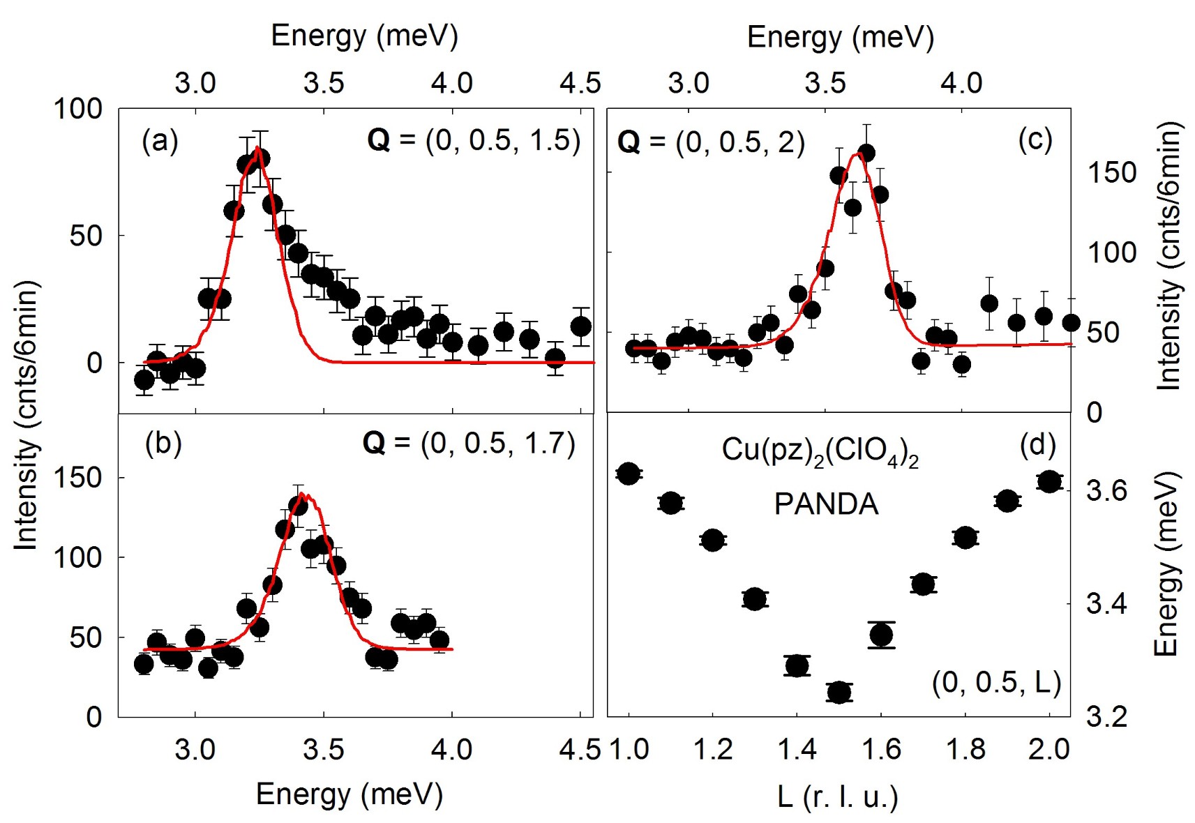
Figure 11: (Color online) (a) The energy scan at $\textbf{Q}=(0,0.5,1.5)$ with the background subtracted as explained in the text. The energy scans performed at wave-vectors $\textbf{Q}=(0,0.5,1.7)$ and $\textbf{Q}=(0,0.5,2)$ are shown in (b) and (c), respectively. The red curves are fits of a Gaussian function convoluted with the resolution function. (d) The antiferromagnetic zone boundary dispersion measured in zero magnetic field and at $\rm T=1.42\;\mathrm{K}$.

IV Conclusions.

We have performed a comprehensive study of the 2D S=1/2 square-lattice AF Cu(pz)₂(ClO₄)₂ using a collection of experimental techniques, including specific heat measurements, neutron diffraction and neutron spectroscopy. The HT phase diagram was mapped out for magnetic fields up to $\rm\mu_{0}H=9T$ applied parallel and perpendicular to the $\rm Cu^{2+}$ square-lattice planes, showing that the HT boundaries of the ordered phase have the same field dependence. This result shows that the dominant exchange interactions between nearest spins are close to the isotropic limit. Applied magnetic fields induces XY spin anisotropy leading to quench of quantum fluctuations, as we observed in the specific heat measurements.

Neutron diffraction confirms the HT phase diagram obtained from macroscopic measurements and extends it up to $\rm\mu_{0}H=13.5\;\mathrm{T}$. The ordered magnetic moment of $\rm Cu^{2+}$ ions at zero field, $\rm m_{0}=0.47(5)\;\mathrm{\mu_{B}}$, is reduced from the expected value, indicating the existence of strong quantum fluctuations in the ground state. Magnetic fields quench quantum fluctuations and significantly increase the size of the ordered magnetic moment to $\rm m_{0}=0.93(5)\;\mathrm{\mu_{B}}$ at $\rm\mu_{0}H=13.5\;\mathrm{T}$. Therefore neutron diffraction confirms the suppression of quantum fluctuations by field-induced anisotropy seen in our specific heat measurements. The study of the ordered magnetic structure by neutron diffraction shows 2D antiparallel alignment of spins at the neighbor sites.

At zero field, we observed a well-defined magnon mode using neutron spectroscopy. Its dispersion is described by the spin Hamiltonian with slightly anisotropic NN interaction with $xy$- and $z$-components equal to $\rm J_{1}^{xy}=1.563(13)\;\mathrm{meV}$, $\rm J_{1}^{z}=0.9979(2)J_{1}^{xy}$ and NNN exchange equal to $\rm J_{2}\simeq 0.02J_{1}^{xy}$. Therefore the closeness of the dominant exchange interaction $\rm J_{1}$ to the isotropic limit measured by neutron spectroscopy explains the similarity of the HT phase diagrams obtained by specific heat measurements in magnetic fields applied parallel and perpendicular to $bc$-plane.

Our results obtained by three different experimental techniques confirm and supplement each other clearly demonstrating that Cu(pz)₂(ClO₄)₂ is the first weakly frustrated 2D S=1/2 AF on a square lattice with the absence of Dzyaloshinsky-Moriya interaction between NN. The measurements verify a relatively large 10.7(4)% zone-boundary dispersion and a rather strong magnetic continuum at the zone boundary. We associate these features with a resonating valence bond fluctuations which are enhanced by a small NNN AF interactions.

V Acknowledgments.

It is a pleasure to thank Dirk Etzdorf and Harald Schneider for technical assistance. This work was supported by the Swiss NSF (Contract No. PP002-102831).

VI Appendix A: The group theory analysis.

	$1$	$2_{b}$	$\overline{1}$	$m_{ac}$
$\Gamma_{1}$	1	1	1	1
$\Gamma_{2}$	1	1	-1	-1
$\Gamma_{3}$	1	-1	1	-1
$\Gamma_{4}$	1	-1	-1	1

Table 2: The character table and the irreducible representations obtained by performing group theory analysis for monoclinic space group C2/c ($\#15$), the table setting choice is b1) and the magnetic ordering vectors $\textbf{k}=(0,0,1)$ and $\textbf{k}=(0,0,0)$.

The crystal structure of Cu(pz)₂(ClO₄)₂ belongs to the monoclinic C2/c space group ($\#15$), whose Laue class and the point group are 2/m. The ${\rm Cu^{2+}}$ ions occupy 4e Wyckoff positions and they are located at $\rm r_{1}=(0\ 0.7499\ 0.25)$, $\rm r_{2}=(0\ 0.2501\ 0.75)$, $\rm r_{3}=(0.5\ 0.2499\ 0.25)$ and $\rm r_{4}=(0.5\ 0.7501\ 0.75)$. For C2/c space group, reciprocal lattice points are located at ${\bf Q}=(h,k,l)$ with $h+k=2n$. The magnetic Bragg peaks were observed at $\textbf{Q}_{1}=(0,1,0)$ and at $\textbf{Q}_{2}=(0,0,1)$ indicating that only $\textbf{Q}_{2}$ can be the magnetic ordering vector. However, taking into account nearly identical crystallographic parameters $b$ and $c$ and the presence of $bc$ and $cb$ crystallographic domains, the magnetic Bragg peaks at $\textbf{Q}_{1}$ and $\textbf{Q}_{2}$ are indistinguishable. Therefore we can not identify whether the magnetic ordering vector is $\textbf{k}=(0,0,1)$ or $\textbf{k}=(0,0,0)$. The subgroups of the ordering wave vectors are identical and consist of four symmetry operations which belong to four different classes: $1$, $2_{b}$,$\overline{1}$ and $m_{ac}$. Here, $1$ is the identity, $2_{b}$ is a two-fold rotation around the b-axis, $\overline{1}$ is the inversion and $m_{ac}$ is a mirror plane in the ac plane. Therefore, there are four one-dimensional irreducible representations whose characters are summarized in the character table given in Tab. 2. The decomposition equation for the magnetic representation is $\rm\Gamma_{mag}=1\Gamma_{1}+1\Gamma_{2}+2\Gamma_{3}+2\Gamma_{4}$. The six basis vectors presented in Tab. 3 are calculated for two $\rm Cu^{2+}$ positions in primitive unit cell using the projection operator method acting on a trial vector $\phi_{\alpha}$

$$\rm\Psi_{\alpha\nu}^{\lambda}=\sum_{g\epsilon G_{k}}D_{\nu}^{\lambda*}(g)\sum_{i}\delta_{i,g_{i}}R_{g}\phi_{\alpha}det(R_{g}),$$

where $\rm\Psi_{\alpha\nu}^{\lambda}$ is the basis vector projected from the $\rm\lambda^{th}$ row of the $\rm\nu^{th}$ irreducible representation, $\rm D_{\nu}^{\lambda*}(g)$ is the $\rm\lambda^{th}$ row of the matrix representative of the $\rm\nu^{th}$ irreducible representation for symmetry operation g, i denotes the atomic position and $\rm R_{g}$ is the rotational part of the symmetry operation g. Note that basis vectors are identical for both $\textbf{k}=(0,0,1)$ and $\textbf{k}=(0,0,0)$.

Dzyaloshinsky-Moriya (DM) interactions are defined as

$$\rm\hat{H}_{DM}=\sum_{\langle i,j\rangle}\ \textbf{D}_{ij}\cdot[\textbf{S}_{i}\times\textbf{S}_{j}],$$

where $\rm\textbf{D}_{ij}$ is an axial vector. Action of any symmetry operation (including lattice translations) $A$ on a DM vector $\rm\textbf{D}_{ij}$ must be equal to $\rm\textbf{D}_{A(i)A(j)}$ and $\rm\textbf{D}_{ij}=-\textbf{D}_{ji}$. We analyze the action of the inversion symmetry operation $\overline{1}$ on the axial DM vector $\rm\textbf{D}_{12}$, where $i=1$ and $j=2$ denotes the NN copper positions $\rm r_{1}=(0\ 0.7499\ 0.25)$ and $\rm r_{2}=(0\ 0.2501\ 0.75)$, respectively. The result of operation is

$$\overline{1}(\rm\textbf{D}_{12})=(D_{12}^{x}\ D_{12}^{y}\ D_{12}^{z}).$$

The application of the inversion symmetry on the ions positions leads to

$$\overline{1}(\rm\textbf{D}_{12})=\rm\textbf{D}_{\overline{1}(1)\overline{1}(2)}=(D_{21}^{x}\ D_{21}^{y}\ D_{21}^{z}).$$

These relations imply $\rm(D_{12}^{x}\ D_{12}^{y}\ D_{12}^{z})=(D_{21}^{x}\ D_{21}^{y}\ D_{21}^{z})$ which is possible only in case of $\rm\textbf{D}_{12}=0$. Therefore, DM interactions between NN in Cu(pz)₂(ClO₄)₂ are forbidden by the crystal symmetry.

VII Appendix B: The linear spin wave theory.

Assuming the system in the antiferromagnetic Nèel ground state with spins pointing along $z$ and $-z$ direction we can make the Holstein-Primakoff transformation of the spin compounds into bosonic creation and annihilation operators. In linear spin wave approximation it gives:

$$\rm S^{z}_{i}=S-a_{i}^{+}a_{i},\ S^{z}_{j}=-S+a_{j}^{+}a_{j},\ S^{z}_{k}=S-a_{k}^{+}a_{k},$$

$$\rm S^{x}_{i}=\sqrt{2S}\ \frac{a_{i}+a_{i}^{+}}{2},\ S^{y}_{i}=\sqrt{2S}\ \frac{a_{i}-a_{i}^{+}}{2i},$$

$$\rm S^{x}_{j}=\sqrt{2S}\ \frac{a_{j}+a_{j}^{+}}{2},\ S^{y}_{j}=\sqrt{2S}\ \frac{-a_{j}+a_{j}^{+}}{2i},$$

$$\rm S^{x}_{k}=\sqrt{2S}\ \frac{a_{k}+a_{k}^{+}}{2},\ S^{y}_{k}=\sqrt{2S}\ \frac{a_{k}-a_{k}^{+}}{2i}.$$

		$X_{1}$	$X_{2}$
$\Gamma_{1}$	$\overrightarrow{\phi}_{1}$	(0 1 0)	(0 1 0)
$\Gamma_{2}$	$\overrightarrow{\phi}_{2}$	(0 1 0)	(0 -1 0)
$\Gamma_{3}$	$\overrightarrow{\phi}_{3}$	(1 0 0)	(1 0 0)
	$\overrightarrow{\phi}_{4}$	(0 0 1)	(0 0 1)
$\Gamma_{4}$	$\overrightarrow{\phi}_{5}$	(1 0 0)	(-1 0 0)
	$\overrightarrow{\phi}_{6}$	(0 0 1)	(0 0 -1)

Table 3: Six basis vectors calculated for two $\rm Cu^{2+}$ positions in primitive unit cell as explained in Appendix A.

The quantization axis lies in $bc$-plane and therefore $\rm J_{1}^{x}=J_{1}^{z}=J,J_{1}^{y}=J-\Delta$. The spin Hamiltonian written in bosonic operators is:

$$\rm\hat{H}=\sum_{\langle i,j\rangle}\{4JS(a_{i}^{+}a_{i}+a_{j}^{+}a_{j})+2S\frac{2J+\Delta}{2}(a_{i}a_{j}+a_{i}^{+}a_{j}^{+})+$$

$$\rm 2S\frac{\Delta}{2}(a_{i}a_{j}^{+}+a_{i}^{+}a_{j})\}+$$

$$\rm\sum_{\langle i,k\rangle}4J_{2}S\{(a_{i}a_{k}^{+}+a_{i}^{+}a_{k})-(a_{i}^{+}a_{i}+a_{k}^{+}a_{k})\},$$

where $\rm\langle i,j\rangle$ indicates the sum over NN in the bc-plane, $\rm\langle i,k\rangle$ - the sum over NNN in the bc-plane. After Fourier transformation obtained Hamiltonian can be diagonalized using standard Bogoliubov transformation:

$$\rm a_{q}=-u_{q}\alpha_{q}+v_{q}\beta_{q}^{+},$$

$$\rm a_{q}^{+}=-u_{q}\alpha_{q}^{+}+v_{q}\beta_{q},$$

$$\rm a_{-q}=v_{q}\alpha_{q}^{+}-u_{q}\beta_{q},$$

$$\rm a_{-q}^{+}=v_{q}\alpha_{q}-u_{q}\beta_{q}^{+},$$

where $\rm\alpha_{q}$ and $\rm\beta_{q}$ are the bosonic operators and $\rm v_{q}$, $\rm u_{q}$ are numbers. Finally, after the diagonalization we have

$$\rm\hat{H}_{q}=E_{g.s.}+\sum_{q}S[2A_{q}\alpha_{q}^{+}\alpha_{q}+B_{q}(\alpha_{q}^{+}\alpha_{-q}^{+}+\alpha_{q}\alpha_{-q})],$$ (2)

and the eigenstates are given by $\rm\hbar\omega_{q}=(A_{q}^{2}-B_{q}^{2})^{1/2}$, where

$$\rm A_{q}=4SJ+S\Delta(\cos(\textbf{qb})+\cos(\textbf{qc}))-$$

$$\rm 4SJ_{2}+4SJ_{2}\cdot\cos(\textbf{qb})\cdot\cos(\textbf{qc})$$

and

$$\rm B_{q}=2S(J-1/2\Delta)(\cos(\textbf{qb})+\cos(\textbf{qc})).$$

References

- (1) F. D. M. Haldane, Phys Lett. A 93, 464 (1983); F. D. M. Haldane, Phys. Rev. Lett. 50, 1153 (1983).
- (2) W. J. L Buyers, R. M. Morra, R. L. Armstrong, M. J. Hogan, P. Gerlach and K. Hirakawa, Phys. Rev. Lett. 56, 371-374 (1986).
- (3) D. A. Tennant, R. A. Cowley, S. E. Nagler and A. M. Tsvelik Phys. Rev. B 52, 13368 (1995).
- (4) R. R. P. Singh and M. P. Gelfand, Phys. Rev. B 52, R15695 (1995).
- (5) A. W. Sandvik, R. R. P. Singh, Phys. Rev. Lett 86, 528 (2001).
- (6) W. Zheng, J. Oitmaa, and C. J. Hamer, Phys. Rev. B 71, 184440 (2005).
- (7) C. M. Ho, V. N. Muthukumar, M. Ogata, and P. W. Anderson, Phys. Rev. Lett. 86, 1626 (2001).
- (8) J. I. Igarashi, Phys. Rev. B 46, 10763 (1992).
- (9) R. R. P. Singh and M. P. Gelfand, Phys. Rev. B 52, R15695 (1995).
- (10) S. J. Clarke, A. Harrison, T. E. Mason, D. Visser, Solid State Commun., 112, 561-564 (1999).
- (11) H. M. Rønnow, D. F. McMorrow, R. Coldea, A. Harrison, I. D. Youngson, T. G. Perring, G. Aeppli, O. Syljuasen, K. Lefmann, and C. Rischel, Phys. Rev. Lett., 87, 037202 (2001).
- (12) A. B. Harris, A. Aharony, O. Entin-Wohlman, I. Ya. Korenblit, R. J. Birgeneau and Y.-J. Kim, Phys. Rev. B 64 024436 (2001).
- (13) N. B. Christensen, D. F. McMorrow, H. M. Ronnow, A. Harrison, T. G. Perring, and R. Coldea, J. Mag. Magn. Mater. 272-276, 896 (2004).
- (14) M. D. Lumsden, S. E. Nagler, B. C. Sales, D. A. Tennant, D. F. McMorrow, S.-H. Lee and S. Park, Phys. Rev. B 74, 214424 (2006).
- (15) N. B. Christensen, H. M. Ronnow, D. F. McMorrow, A. Harrison, T. G. Perring, M. Enderle, R. Coldea, L. P. Regnault and G. Aeppli, Proc. Natl. Acad. Sci. U.S.A., Vol. 104 (39), pp. 15264-15269 (2007).
- (16) R. Coldea, S. M. Hayden, G. Aeppli, T. G. Perring, C. D. Frost, T. E. Mason, S.-W. Cheong, and Z. Fisk, Phys. Rev. Lett. 86, 5377 (2001).
- (17) P. Chandra and B. Doucot, Phys. Rev. B 38, 9335 (1988).
- (18) P. Chandra, P. Coleman and A. I. Larkin, Phys. Rev. Lett. 64, 88 - 91 (1990).
- (19) N. Read and S. Sachdev, Phys. Rev. Lett. 66, 1773 (1991).
- (20) J. R. Viana and J. R. de Sousa, Phys. Rev. B 75, 052403 (2007).
- (21) N. Tsyrulin, T. Pardini, R. R. P. Singh, F. Xiao, P. Link, A. Schneidewind, A. Hiess, C. P. Landee, M. M. Turnbull, and M. Kenzelmann, Phys. Rev. Lett., 102, 197201 (2009).
- (22) F. M. Woodward, P. J. Gibson, G. Jameson, C. P. Landee, M. M. Turnbull and R. D. Willett, Inorg. Chem., 46, 4256-4266 (2007).
- (23) T. Lancaster, S. J. Blundell, M. L. Brooks, P. J. Baker, F. L. Pratt, J. L. Manson, M. M. Conner, F. Xiao, C. P. Landee, F. A. Chaves, S. Soriano, M. A. Novak, T. P. Papageorgiou, A. D. Bianchi, T. Herrmannsdörfer, J. Wosnitza, J. A. Schlueter, Phys. Rev. B 75, 094421 (2007).
- (24) F. Xiao, F. M. Woodward, C. P. Landee, M. M. Turnbull, C. Mielke, N. Harrison, T. Lancaster, S. J. Blundell, P. J. Baker, P. Babkevich, F. L. Pratt, Phys. Rev. B 79, 134412 (2009).
- (25) A. Cuccoli, T. Roscilde, R. Vaia, and P. Verrucchi, Phys. Rev. B 68, 060402(R) (2003).
- (26) V. L. Berezinskii, Sov. Phys. JETP 32, 493 (1971).
- (27) J. M. Kosterlitz and D. J. Thouless, J. Phys. C 6, 1181 (1973).
- (28) A. L. Chernyshev, Phys. Rev. B, 72, 174414 (2005)