Geographical networks stochastically constructed
by a self-similar tiling according to population

Abstract

In real communication and transportation networks, the geographical positions of nodes are very important for the efficiency and the tolerance of connectivity. Considering spatially inhomogeneous positions of nodes according to a population, we introduce a multi-scale quartered (MSQ) network that is stochastically constructed by recursive subdivision of polygonal faces as a self-similar tiling. It has several advantages: the robustness of connectivity, the bounded short path lengths, and the shortest distance routing algorithm in a distributive manner. Furthermore, we show that the MSQ network is more efficient with shorter link lengths and more suitable with lower load for avoiding traffic congestion than other geographical networks which have various topologies ranging from river to scale-free networks. These results will be useful for providing an insight into the future design of ad hoc network infrastructures.

I INTRODUCTION

Since the common topological characteristics called small-world (SW) and scale-free (SF) have been revealed in social, technological, and biological networks, researches on complex networks have attracted much attention in this decade through the historical progress Newman06 . The topological structure is quite different from the conventionally assumed regular and random graphs, and has both desirable and undesirable properties: short paths counted by hops between any two nodes and the fault-tolerance for random node removals Cohen00 ; Albert00 on the one hand but the vulnerability against intentional attacks on hubs Albert00 ; Callaway00 on the other hand. In the definition of a network, spatial positions of nodes and distances of links are usually ignored, these simplifications are reasonable in some networks such as the World-Wide-Web, citation networks, and biological metabolic networks. However, as real-life infrastructures, in communication networks, transportation systems, and the power grid, they are crucial factors; a node is embedded in a mixing of sparse and dense areas according to the population densities, and a connection between nodes depends on communication efficiency or economical cost. Thus, a modeling of geographical networks is important to understand the fundamental mechanism for generating both topological and spatial properties in realistic communication and transportation systems.

Many methods for geographically constructing complex networks have been proposed from the viewpoints of the generation mechanism and the optimization. As a typical generation mechanism, a spatially preferential attachment is applied in some extensions Brunet02 ; Manna02 ; Manna03 ; Nandi07 ; Wang09 of the Barabási-Albert (BA) model Barabasi99 . As typical optimizations in the deterministic models Qian09 ; Zhou07 ; Barthelemy06 ; Gastner06b , there are several criteria for maximizing the traffic under a constraint Qian09 , minimizing a fraction of the distance and node degree with an expectation of short hops Zhou07 , and minimizing a sum of weighted link lengths w.r.t the edge betweenness as the throughput Barthelemy06 or the forwarding load at nodes Gastner06b . In these methods, various topologies ranging from a river network to a SF network emerge according to the parameter values. The river network resembles a proximity graph known in computer science, which has connections in a particular neighbor relationship between nodes embedded in a plane. In constructing these networks, it is usually assumed that the positions of nodes are distributed uniformly at random, and that a population density or the number of passengers is ignored in communication or transportation networks except in some works Nandi09 ; Gastner06b ; Barthelemy06 . However, in real data Yook02 , a population density is mapped to the number of router nodes on Earth, the spatial distribution of nodes does not follow uniformly distributed random positions represented by a Poisson point process. Such a spatially inhomogeneous distribution of nodes is found in air transportation networks Guimera05 and in mobile communication networks Lambiotte08 .

On the other hand, geometric methods have also been proposed as another generation mechanism, in which both SW and SW structures are generated by a recursive growing rule for the division of a chosen triangle Zhang08 ; Zhou05 ; Zhang06 ; Doye05 or for the attachment aiming at a chosen edge Wang06 ; Rozenfeld06 ; Dorogovtsev02 in random or hierarchical selection. The position of a newly added node is basically free as far as the geometric operations are possible, and has no relation to a population. Thus, the spatial structure with geographical constraints on nodes and links has not been investigating enough. In particular, considering the effects of a population on a geographical network is necessary to self-organize a spatial distribution of nodes that is suitable for socio-economic communication and transportation requests.

In this paper, as a possibility, we pay attention to a combination of complex network science and computer science (in particular, computational geometry and routing algorithm) approaches. This provides a new direction of research on self-organized networks by taking into account geographical densities of nodes and population. We consider an evolutionary network with a spatially inhomogeneous distribution of nodes based on a stochastic point process. Our point process differs from the tessellations for a Voronoi partitioning with different intensities of points Blaszczyszy04 and for a modeling of crack patterns Nagel07 . We aim to develop a future design method of ad hoc networks, e.g., on a dynamic environment which consists of mobile users, for increasing communication requests, and wide-area wireless and wired connections. More precisely, the territory of a node defined as the nearest access point is iteratively divided for load balancing of communication requests which are proportional to a population density in the area. A geographical network consisting of a self-similar tiling is constructed by recursive subdivision of faces according to a population. It is worth noting that positions of nodes and a network topology are simultaneously decided by the point process in a self-organized manner. Furthermore, the geographical network has several advantages Hayashi09 : the robustness of connectivity, the short path lengths, and the decentralized routing algorithm Bose04 . Taking these advantages into consideration, we generalize the point process biased by a population for constructing a geographical network, and investigate the traffic load on the shortest distance routing.

The organization of this paper is as follows. In Sec. II, we introduce a more general network model for self-similar tilings than the previous model Hayashi09 based on triangulations. By applying the geometric divisions, we construct a geographical network according to a given population. In Sec. III, we show the properties of the shortest path and the decentralized routing without a global table for packet transfers as applied in the Internet. We numerically investigate the traffic load in the proposed network, comparing it with the load in other geographical networks. In particular, we show that our geographical network is better than the state-of-the-art geographical networks in terms of shorter paths and link lengths, and of lower load for avoiding traffic congestion. In Sec. IV, we summarize the results and briefly discuss further studies.

II MSQ NETWORK MODEL

We introduce a multi-scale quartered (MSQ) network, which is stochastically constructed by a self-similar tiling according to a given population. Let us consider the basic process of network construction Hayashi09 . Each node corresponds to a base station for transferring packets, and a link between two nodes corresponds to a wireless or wired communication line. Until a network size $N$ is reached, the following process is repeated from an initial configuration which consists of equilateral triangles or squares. At each time step, a triangle (or square) face is chosen with a probability proportional to the population in the space of the triangle (or square). Then, as shown in Figs. 1(a) and 1(b), four smaller triangle (or square) faces are created by adding facility nodes at the intermediate points on the communication links of the chosen triangle (or square). This process can be implemented autonomously for a division of the area with the increase of communication requests. Thus, a planar network is self-organized on a geographical space. Figure 2 shows an example of the geographical MSQ network according to real population data. If we ignore the reality for a distribution of population, the MSQ network includes a Sierpinski gasket obtained by a special selection when each triangle, except the central one, is hierarchically divided.

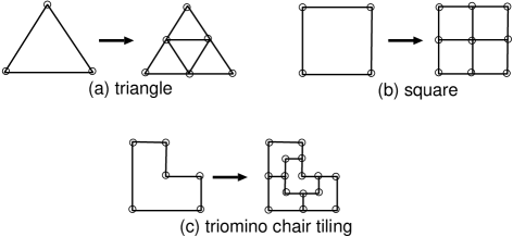
Figure 1: Basic process of the division.

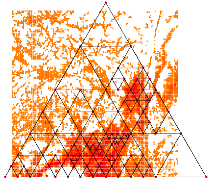
Figure 2: (Color online) Example of the proposed geographical network. The mesh data of population statistics (consisting of $8^{2}\times 10^{2}\times 4=25600$ blocks for $80{\rm km}^{2}$) provided by the Japan Statistical Association are mapped onto each triangle by counting the number of people in the space. From light (orange) to dark (red), the gradation on a mesh block is proportionally assigned to the population. In the middle of the main island of Japan, almost all of the blocks consist of flat lands and mountains, and do not come in contact with the sea except in the left bottom curved white area.

The state-of-the-art geometric growing network models Zhang08 ; Wang06 ; Rozenfeld06 ; Dorogovtsev02 ; Zhou05 ; Zhang06 ; Doye05 are summarized in Table 1. The basic process for network generation is based on the division of a triangle or on the extension of an edge with a bypass route as shown in Fig. 3. For these models, we can also consider a mixing of dense and sparse areas of nodes by selecting a triangle or an edge according to a population in the territory. Although the geographical position of a new node has not been so far exactly defined in the geometric processes, it is obviously different from that in the MSQ network. Moreover, in the Pseudofractal SF network Wang06 , the link length tends to be longer than that in the MSQ network, because a node is set freely at an exterior point. Whereas the newly added three nodes approach each other in the Sierpinski network Zhang08 as the iteration progresses, they are degenerated (shrunken) to one node as in the random Apollonian network Zhou05 ; Zhang06 . Thus, we focus on the Apollonian network constructed by a biased selection of a triangle according to a population. In Sec. III, we compare the topological and the routing properties in the BA-like and the Apollonian networks with those in the MSQ network.

The above geometric models generate SF networks whose degree distribution follows a power-law. It is known that a SF network is extremely vulnerable against intentional attacks on hubs Callaway00 ; Albert00 , in particular the tolerance of connectivity is more weakened by geographical constraints on linking Hayashi06 . However, the MSQ network without high degree nodes has a quite different property. The MSQ network consists of trimodal low degrees: $k_{1}=2$, $k_{2}=4$, and $k_{3}=6$ for an initial triangle ($k_{2}=3$, and $k_{3}=4$ for an initial square) configuration. Because of the trimodal low degrees without hubs, the robustness against both random failures and intentional attacks is maintained Hayashi09 at a similar level as the optimal bimodal networks Tanizawa06 with a larger maximum degree $k_{2}=O(\sqrt{N})$ in a class of multimodal networks, which include a SF network at the maximum modality $\rightarrow\infty$ as the worst case for the robustness.

In the MSQ network, the construction method defined by recursive subdivision of equilateral triangles or squares can be extensively applied to self-similar tilings based on polyomino Keating99 , polyiamond Solomyak97 , and polyform MathWorld , as shown in Fig. 1(c). In the general construction on a polygon, some links are removed from the primitive tiling which consists of equilateral triangles or squares in order to be a specially shaped face such as a “sphinx” or “chair” at each time step of the subdivision. It remains to be determined whether or not the robustness of connectivity is weaker than that in our geographical networks based on equilateral triangles or squares. However, the path length becomes larger at least, as mentioned in Sec. III A.

Model	Structure	Add new node(s)	Selection
MSQ	Trimodal	On the edges of	According to
	low degrees	a chosen triangle	a population
		(or square)
Random	SF, SW,	Mapped to the edges	RandomZhang08
Sierpinski	modular	of a removed triangle
		in a Sierpinski gasket
Apollonian	SF, SW	Interior of a chosen	RandomZhou05 ; Zhang06 or
		triangle	hierarchical
			deterministicZhou05 ; Doye05
Pseudofractal	SF, SW	Exterior attached to	RandomWang06 or
SF		both ends of an edge	hierarchical
		or replacing	deterministicRozenfeld06 ; Dorogovtsev02
		each edge	by two parallel paths

Table 1: Geometically constructed network models.

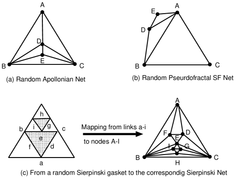
Figure 3: Other geometric networks. From an initial triangle ABC, the following processes are repeated. (a) At each time step, a triangle is randomly chosen. Then, a new node is added (e.g., at the barycenter as a well-balanced position) and connected to the three nodes of the chosen triangle for the division. (b) Instead of a triangle, an edge is randomly chosen. Then, a new node is added at an exterior point, and connected to the two ends of the chosen edge. (c) After a random selection of a triangle, it is divided into small ones, and the center (shaded part) is removed to construct a random Sierpinski gasket. Then, the corresponding random Sierpinski network is obtained from the mapping of nodes and contacts to links between them. Note that the Sierpinski network has a similar structure to the Apollonian network rather than the Sierpinski gasket.

III ROUTING PROPERTIES

III.1 Bounded shortest path

The proposed MSQ network becomes the $t$-spanner Karavelas01 , as a good graph property known in computer science: the length of the shortest distance path between any nodes $u$ and $v$ is bounded by $t$ times the direct Euclidean distance $d_{uv}$. A sketch of the proof is shown in the Appendix. Here, $t$ is called stretch factor which is defined by a ratio of the path length (a sum of the link lengths on the path) to $d_{uv}$. Figure 4 shows typical cases of the maximum stretch factor $t=2$ in the MSQ network Hayashi09 . When the unit length is defined by an edge of the biggest equilateral triangle (or square), the path length denoted by a dashed line in Fig. 4 is 1 (or 2) while the direct Euclidean distance between the two nodes is 1/2 (or 1).

More generally, if we construct a network by recursive subdivision to a self-similar tiling of a polyform MathWorld , e.g., polydrafter: consisting of right triangles, polyabolo: consisting of isosceles right triangles, or domino: consisting of rectangles, then the stretch factor can be greater than $2$ [see the U-shaped path in the right of Fig. 1(c)]. Thus, our network model based on equilateral triangles or squares is better for realizing a short routing path because of its isotropic property. In other geometric graphs, the maximum stretch factor becomes larger: $t=2\pi/[3\cos(\pi/6)]\approx 2.42$ for Delaunay triangulations Keil92 , and $t=2\alpha\geq 4\sqrt{3}/3\approx 2.3094$ for two-dimensional triangulations with an aspect ratio of hypotenuse/height less than $\alpha$ Kranakis06 , whose lower bound is given for the fattest equilateral triangles. Although $\Theta$-graphs Farshi05 with $K$ non-overlapping cones have $t=1/[\cos(2\pi/K)-\sin(2\pi/K)]\rightarrow 1$ asymptotically as $K\rightarrow\infty$, a large amount of $O(KN)$ links is necessary, and some links may be crossed. In general graphs, even the existence of a bounded stretch factor is uncertain. On the other hand, in a SF network, the efficient routing Carmi06 based on the passing through hubs has a stretch less than 2, which is defined by the ratio of the number of hops on the routing path to that on the shortest path. It can be implemented by a decentralized algorithm within small memory requirements.

Since the geographical MSQ network is planar, which is also suitable for avoiding the interference among wireless beams, we can apply an efficient routing algorithm Bose04 using only local information of the positions of nodes: neighbors of a current node, the source, and the terminal on a path. The online version has been developed in a distributive manner, in which necessary information for the routing is gathered through an exploration within a constant memory. As shown in Fig. 5, by using the face routing, the shortest distance path can be found on the edges of the faces that intersect the straight line between the source and the terminal nodes. Note that, in other decentralized routings without global information such as a routing table, some of them in early work lead to the failure of guaranteed delivery Urrutia02 ; e.g., in the flooding algorithm, multiple redundant copies of a message are sent and cause network congestion, while greedy and compass routings may occasionally fall into infinite loops. On a planar graph, the face routing has advantages for the guarantee of a delivery and for the efficient search on a short path without the flooding.

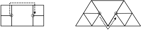
Figure 4: Cases of the maximum stretch factor $t=2$ for the shortest distance path denoted by a dashed line and the straight line directly passing the gap between two nodes marked by circles.

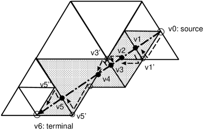
Figure 5: The shortest path obtained by the face routing on the edges of the shaded triangles that intersect the straight line between the source and the terminal nodes. Two paths of dashed segments in the opposite directions (for $v1$-$v1^{\prime}$ and $v3$-$v3^{\prime}$) are canceled, therefore the route does not pass the points $v_{1}$ and $v_{3}$, and through only the other nodes (marked by open circles) on the triangles. Exceptionally, it takes the shortcut $v5^{\prime}$-$v6$ to avoid the detour passing through $v_{5}$ and $v_{5^{\prime\prime}}$.

III.2 Comparison of $P(k)$ and $P(L_{ij})$ with other networks

We investigate the distributions of degree and of link length related to communication costs. In the following BA-like networks, the positions of nodes are fixed as same as in the original MSQ network, and only the connections are different. From the set of nodes in the MSQ network, a node is randomly selected as the new node at each time step in the growing process. On the other hand, the positions of nodes in the Apollonian network are different from the original ones because of the intrinsic geometric construction.

Let us consider an extension of the BA model with both effects of distance Brunet02 ; Manna02 ; Manna03 ; Nandi07 ; Wang09 and population on linking. Until a size $N$ is reached, at each time step, $m$ links are created from a new node $i$ to already existing nodes $j$. The attachment probability is given by

$$\Pi_{j}\propto d_{ij}^{-\alpha}pop_{j}^{\beta}k_{j}^{\gamma},$$ (1)

where $\alpha,\beta,\gamma\geq 0$ are parameters to control the topology Nandi07 ; Zhou07 , $k_{j}$ denotes the degree of node $j$, and $d_{ij}$ denotes the Euclidean distance between nodes $i$ and $j$. The newly introduced term $pop_{j}$ is not constant but may vary through time. If the nearest node from a point on the geographical space is changed by adding a new node, then the assigned population $pop_{j}$ in the territory of the affected node $j$ is updated. We set the average degree $\langle k\rangle=2m=4$ that is the closest integer to $\langle k\rangle$ in the MSQ network.

Each term in the right-hand side of Eq. (1) contributes to making a different topology, as the value of $\alpha$, $\beta$, or $\gamma$ is larger in the competitive attachments. As shown in Fig. 6, a proximity graph is obtained in the BA-like:300,330 networks by the effect of distance for $\alpha=3$, and hubs emerge near large cities in the BA-like:030,033,333 networks by the effect of population for $\beta=3$, while in the BA-like:303,003 networks, a few hubs emerge at the positions of randomly selected nodes in the early stage of network generation without any relation to the population. In the following discussion, we focus on BA-like:300,033 networks, since they are typical with the minimum and the maximum degrees or link lengths, respectively, in the combination of $\alpha\beta\gamma$ except 000,003 without both effects of distance and population. Figure 7(a) shows that the degree distributions $P(k)$ follow an exponential decay in the BA-like:300 network, and a power-law like behavior in the BA-like:033 and the Apollonian networks, which are denoted by a (red) solid line, (green) light dashed line, and (blue) dark dotted line, respectively. Figure 7(b) shows the distributions $P(L_{ij})$ of link length counted as histograms in the interval 0.05. The $L_{ij}$ is normalized by the maximum length on the outer square or triangle. Some long-range links are remarkable in the BA-like networks, while they are rare in the quickly decaying distribution in the MSQ network. The average lengths shown in Table 2 are around $0.2\sim 0.3$ in many cases of the BA-like networks, and $0.02\sim 0.14$ in the Apollonian network. The original MSQ network has the smallest link length in less than one digit. As the size $N$ increases, the link lengths tend to be shorter due to a finer subdivision in all of the networks. In any case, the BA-like networks have longer links even with neighboring connections than the corresponding MSQ network, while the Apollonian network shows the intermediate result. Thus, the MSQ network is better than the Apollonian and the BA-like networks in term of the link length related to a communication cost.

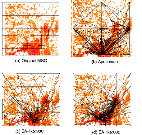
Figure 6: (Color online) Visualizations of the original MSQ, the Apollonian, and the typical BA-like networks for $N=100$. As a common feature, many nodes concentrate on dark cloudy (red) areas with large populations. The positions of nodes are same in the MSQ and the BA-like networks, while they are slightly different in the Apollonian network. (b) Remarkable hubs exist at the center and four points on the outer lines. (c) Almost nearest connections are constructed by the attachment of distance. (d) Hubs emerge near large cities in the dark cloudy (red) areas: Kobe, Osaka, and Kyoto by the attachments of population and degree. These results with the nearest connections and hubs are similarly obtained in other combinations of $\alpha\beta\gamma$ for BA-like networks. Here, 0 or 3 in the triplet denotes the parameter values for $\alpha$, $\beta$, and $\gamma$ in Eq. (1).

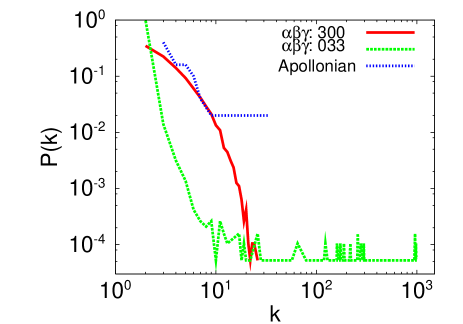
(a) Degree

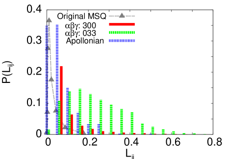
(b) Link length

Figure 7: (Color online) Distributions of (a) degree and (b) link length in the averaged 50 realizations of the Apollonian and the typical BA-like networks for $N=1000$. (a) With power-law like behavior, there exists a few huge hubs around $k=10^{2}\sim 10^{3}$ at the vertical (green) light dashed bars for the BA-like:033 network, and ordinary hubs on the horizontal (blue) dark dotted line for the Apollonian network. In spite of the stochastic process, the locations of hubs are fixed e.g., at the center and four points on the outer lines in Fig.6(b). Thus, the frequencies are high at some special degrees. (b) The histograms are shown with shifts for better discrimination. The gray dashed lines with filled triangles show $P(L_{ij})$ in the original MSQ network.

BA-like:		$\langle L_{ij}\rangle$		Dominant
$\alpha\beta\gamma$	$N=10^{2}$	$10^{3}$	$10^{4}$	factor
000	0.3018	0.2380	0.1909	Rand. attach.
003	0.2757	0.2736	0.1700	Degree
030	0.2759	0.2651	0.2318	Population
033	0.2685	0.2650	0.2622	Pop. & deg.
300	0.1268	0.0436	0.0213	Distance
303	0.2089	0.1409	0.1127	Dist. & deg.
330	0.1789	0.0652	0.0338	Dist. & pop.
333	0.2318	0.2064	0.1613	All of them
Apollonian	0.1401	0.0627	0.0184
MSQ	0.0628	0.0066	0.0033

Table 2: Average link length $\langle L_{ij}\rangle$ in the original MSQ, the Apollonian, and the BA-like networks. The $\langle L_{ij}\rangle$ becomes longer in the order: the MSQ, the BA-like:300 or the Apollonian, and the BA-like:033 networks. This order is consistent with the positions of peaks and the widths of $P(L_{ij})$ in Fig. 7(b). Note that BA-like:000,003 networks are not geographical, but exceptional, because they have no effects of distance and population on linking. Here, the triplet of 0 or 3 in the first column denotes the values of $\alpha$, $\beta$, and $\gamma$.

III.3 Heavy-loaded nodes and links

In a realistic situation, packets are usually more often generated and received at a node, as the corresponding population is larger in the territory of the node. Consequently, the spatial distribution of the source or the terminal node is not uniformly random. Thus, we demonstrate how the traffic load is localized in the case when the number of generated and received packets at a node varies depending on a population assigned to the node.

The traffic loads at a node $i$ and through a link $l$ are measured by the effective betweenness centralities $B_{i}$ and $\bar{B}_{l}$, which are defined as follows Guimera02 :

$$B_{i}\stackrel{{\scriptstyle\rm def}}{{=}}\frac{2}{(N-1)(N-2)}\sum_{k<j}\frac{b_{k}^{j}(i)}{b_{k}^{j}},$$ (2)

$$\bar{B}_{l}\stackrel{{\scriptstyle\rm def}}{{=}}\frac{2}{(N-1)(N-2)}\sum_{k<j}\frac{\bar{b}_{k}^{j}(l)}{b_{k}^{j}},$$ (3)

where $b_{k}^{j}$ is the number of shortest distance paths between the source $k$ and the terminal $j$, $b_{k}^{j}(i)$ is the number of the paths passing through node $i$, and $\bar{b}_{k}^{j}(l)$ is the number of the paths passing through link $l$. The first terms on the right-hand side of both Eqs. (2) and (3) are normalization factors. Although the measured node $i$ and link $l$ are usually excluded from the sum in the definition of betweenness centralities Freeman91 , we include them tanking into account the processes for the generation and the removal of a packet in these measures $B_{i}$ and $\bar{B}_{l}$ in order to investigate all of the traffic loads.

Figures 8 and 9 show the link load measured by $\bar{B}_{l}$ for the following two selection patterns of packet generations or removals. In the first pattern denoted by Pop, as the source or the terminal, a node is chosen with a probability proportional to the assigned population to the node (left figures), while in the second pattern denoted by Rand, it is chosen uniformly at random (right figures). Therefore, the sum in Eqs. (2) or (3) has a biased frequency for each pair of nodes by their populations in Pop, while the sum corresponds to the simple combination of nodes in Rand. In Pop, heavy-loaded links denoted by thick (blue) lines between the cloudy (red) areas with large populations are observed: the routes between well-known cities Osaka and Kyoto (in the enclosed bold lines) are remarkable with thicker (blue) links than in Rand. Note that the number $N=100$ of nodes is due to a comparatively clear appearance of the difference in two patterns. At a larger $N$, the packet transfer is already biased by the spatial concentration of nodes, and the assigned population in each territory of node is well-balanced by the division process. Then, the difference of heavy-loaded links in Rand and Pop tends to disappear. However, it is worth considering such biased selections of packets in a realistic problem setting, since the spatially localized positions of the heavy-loaded links are not trivially predictable from the results for the usually assumed Rand.

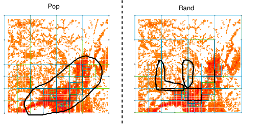
Figure 8: (Color online) Visualizations of the link betweenness centrality $\bar{B}_{l}$ in a MSQ network for $N=100$. Pop (left) and Rand (right) denote the selection patterns of a source or a terminal node, which are chosen proportionally to the population in the territory of a node, and uniformly at random, respectively. From the thin (green) to the thick (blue) vertical or horizontal line, the gradation is proportionally assigned to the value of $\bar{B}_{l}$. The enclosed bold line in Pop emphasizes the parts of large $\bar{B}_{l}$ with heavy load, which are remarkably shown as thick (blue) links on the paths connected to dark cloudy (red) areas with large populations in a diagonal direction. The enclosed bold lines in Rand emphasize the thick (blue) lines on light gray (orange and white) background for underpopulated areas, as the other differences between the left and the right figures. Thus, in Rand, some thick (blue) lines for large $\bar{B}_{l}$ have no relation to the population.

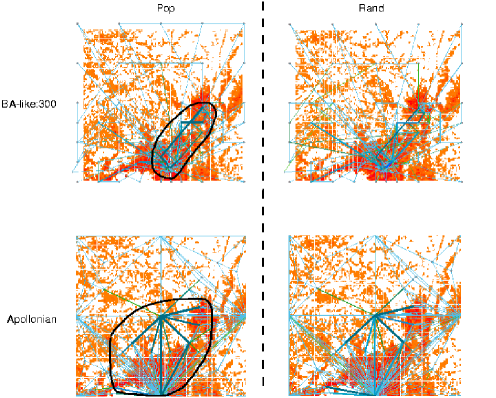
Figure 9: (Color online) Visualized examples of the link betweenness centrality $\bar{B}_{l}$ in the BA-like:300 (top) and the Apollonian (bottom) networks for $N=100$. The enclosed bold line in Pop emphasizes that the thick (blue) links for large $\bar{B}_{l}$ are on the paths connected to dark cloudy (red) areas with large populations. Pop (left) and Rand (right) denote the two selection patterns of a source or a terminal node which is chosen proportionally to the population assigned to a node, and uniformly at random, respectively.

We further investigate the maximum betweenness in the scaling relation $N^{\delta}$ which affects traffic congestion Sreenivasan07 . Here, the betweenness is defined by the number of passings through a link or a node on the shortest distance paths. In general, a smaller $\delta$ yields a better performance for avoiding traffic congestion. The exponent value $\delta$ depends on both a network topology and a routing scheme. In this paper, assuming the shortest distance paths obtained by the face routing in Sec.IIIA, we focus on an effect of the topologies on the scaling relations in the MSQ, the Apollonian, and BA-like networks.

Figure 10 shows the scaling relations of the maximum node betweenness. They are separated into two groups of $\delta=1.67\sim 1.77$ and $\delta=1.87\sim 1.97$. The MSQ network with only trimodal low degrees is located on the baseline. The order of thick lines from the bottom to the top fairly corresponds to the increasing order of largest degrees in these networks, as shown in Fig. 7(a), because more packets tend to concentrate on large degree nodes as the degrees are larger. Figure 11 shows the scaling relations of the maximum link betweenness. The thick lines from the top to the bottom in the inverse order to that in Fig. 10 show that packets are distributed on many links connected to large degree nodes as the degrees are larger. However, all lines lie almost around the intermediate slopes of $\delta=1.6$, especially for a large size $N$, the maximum link load is at a similar level in the lowest case of the Apollonian network and the hightest case of the BA-like:300 or the MSQ network. These results in Figs. 10 and 11 are also consistent with the increasing orders of the maximum $B_{i}$ and $\bar{B}_{l}$ in Table 3. Note that there exists no remarkable difference between the two patterns of Rand (marked by triangles) and Pop (marked by inverted triangles) for both scaling relations of node and link loads except in the Apollonian network (dashed-dotted line). In summary, the MSQ network yields a better performance with a lower maximum load than the other geographical networks, therefore it is more suitable for avoiding traffic congestion.

Figure 10: Scaling relations $N^{\delta}$ of the maximum node betweenness in the MSQ (solid line), BA-like:300 (dotted line), the Apollonian (dashed-dotted line), and the BA-like:033 (dashed line) networks. The triangle and inverted triangle marks correspond to Pop and Rand, respectively. The thin lines without any marks guide the slopes $\delta=1.67,1.77,1.87,1.97$ from the bottom to the top.

Figure 11: Scaling relations $N^{\delta}$ of the maximum link betweenness in the MSQ, the BA-like, and the Apollonian networks. The thick lines and marks are the same as in Fig. 10. The thin lines without any marks guide the slopes $\delta=1.5,1.6,1.7$ from the bottom to the top.

	Rand	Pop	Rand	Pop
Net	Max $B_{i}$	Max $B_{i}$	Max $\bar{B}_{l}$	Max $\bar{B}_{l}$
000	0.254	0.227	0.085	0.081
003	0.766	0.854	0.048	0.087
030	0.362	0.392	0.134	0.180
033	0.657	0.710	0.056	0.099
300	0.282	0.235	0.121	0.121
303	0.444	0.532	0.073	0.107
330	0.397	0.337	0.121	0.143
333	0.634	0.620	0.106	0.072
Apollonian	0.295	0.278	0.056	0.059
MSQ	0.227	0.259	0.137	0.185

Table 3: Maximum betweenness centralities in the BA-like, the Apollonian, and the MSQ networks for $N=100$. The triplet of 0 or 3 in the first column denotes the values of $\alpha\beta\gamma$ in the BA-like networks. We note that the MSQ, the BA-like:300, the Apollonian, and the BA-like:033 networks are in increasing order of max $B_{i}$ and decreasing order of max $\bar{B}_{l}$.

IV CONCLUSION

Both mobile communication and wide-area wireless technologies (or high-speed mass mobilities) are important more and more to sustain our socio-economic activities, however it is an issue to construct an efficient and robust network on the dynamic environment which depends on realistic communication (or transportation) requests. In order to design the future ad hoc networks, we have considered geographical network constructions, in which the spatial distribution of nodes is naturally determined according to a population in a self-organized manner. In particular, the proposed MSQ network model is constructed by a self-similar tiling for load balancing of communication requests in the territories of nodes. On a combination of complex network science and computer science approaches, this model has several advantages Hayashi09 : the robustness of connectivity, the bounded short paths, and the efficient decentralized routing on a planar network. Moreover, we have numerically shown that the MSQ network is better in term of shorter link lengths than the geographical Apollonian and the BA-like networks which have various topologies ranging from river to SF networks. As regards the traffic properties in the MSQ network, the node load (defined by the maximum node betweenness) is lower with a smaller $\delta$ in the scaling relation $N^{\delta}$, although the link load is at a similar level as that of the other geographical networks. Therefore, the MSQ network is more tolerant to traffic congestion than the state-of-the-art geographical network models.

In a realistic situation, packets are usually more often generated and received at a node whose population is large in the territory. Thus, we take into account spatially inhomogeneous generations and removals of packets according to a population. Concerning the effect of population on the traffic load, the heavy-loaded routes with much throughput of packets are observed between large population areas especially for a small size $N$. The heavy-loaded parts are not trivial but localized depending on the geographical connection structure, whichever a spatial distribution of nodes or biased selections of the source and the terminal is more dominant. In further studies, such spatially biased selections of packets should be investigated more to predict overloaded parts on a realistic traffic, since the selections may depend on other economic and social activities in tradings or community relationships beyond the activities related only to population, and probably affect the optimal topologies for the traffic Barthelemy06 ; Qian09 ; Nandi09 . The optimal routing Sreenivasan07 instead of our shortest distance routing is also important for reducing the maximum betweenness ($B_{i}$ or $\bar{B}_{l}$) and the exponent $\delta$ in the scaling relation. In the optimizations that include other criteria Wang09 ; Gastner06b , we will investigate the performance of the MSQ networks. Related discussions to urban street networks Cardillo06 ; Masucci09 ; Bitner09 are attractive for investigating a common property which has arisen from the geographically pseudofractal structures.

Appendix

We provide a sketch of the proof for the $t$-spanner property in the MSQ networks. The following is similarly discussed for other polygons by exchanging the term “triangle” or “triangulation” with other words (e.g., “square” or “polygonal subdivision”), except that the maximum stretch factor $t$ may be greater than two for a general polygon. Remember that the self-similar tiling is obtained from the division by a contraction map as shown in Fig. 1.

Let ${\cal T}$ be a given triangulation and $L_{st}$ be a line segment interconnecting two vertices $so$ and $te$ in ${\cal T}$. It intersects many triangle faces in ${\cal T}$. Let $(so=v_{0},v_{1},\ldots,v_{n}=te)$ be those ordered vertices. Now, we define a path using triangular edges. For any two consecutive vertices $v_{i}$ and $v_{i+1}$ there is a unique triangle which contain both of them. In other words, $v_{i}$ and $v_{i+1}$ are the entrance and the exit of the line segment to the triangle. For the pair $(v_{i},v_{i+1})$ there are two paths, clockwise and anticlockwise, on the triangle. We take the shorter one. In this way, we can define a path on the given triangulation. If the path contains duplicated segments with the opposite directions as shown in Fig. 5, we remove them. Then, we have a path such that each edge of the path is some triangular side. When the two consecutive edges on the path belong to the links of a same triangle, we take a shortcut by directly passing another edge (see two edges $v5^{\prime}$-$v5^{\prime\prime}$ and $v5^{\prime\prime}$-$v6$ are replaced with $v5^{\prime}$-$v6$ on the path in Fig.5). Since ${\cal T}$ is planar and there is no node inside each triangle, the length of this path is the closest to that of the line segment $L_{st}$, therefore the shortest in all other routes. As is easily seen, in each triangle, the path length between $v_{i}$ and $v_{i+1}$ is at most twice longer than the Euclidean distance between them. The worst case of the maximum stretch factor $t=2$ is illustrated in Fig. 4.

References

- (1) M.E.J. Newman, A.-L. Barabási, and D.J. Watts, The Structure and Dynamics of NETWORKS, (Princeton University Press, Princeton, NJ, 2006).
- (2) R. Cohen, K. Erez, D. ben-Avraham, and S. Havlin, Phys. Rev. Lett. 85, 4626, (2000).
- (3) R. Albert, H. Jeong, and A.-L. Barabási, Nature(London) 406, 378, (2000).
- (4) D.S. Callaway, M.E.J. Newman, S.H. Strogatz, and D.J. Watts, Phys. Rev. Lett. 85, 5468, (2000).
- (5) A.K. Nandi, and S.S. Manna, New J. Phys. 9, 30, (2007).
- (6) R. Xulvi-Brunet, and I.M. Sokolov, Phys. Rev. E 66, 026118, (2002).
- (7) S.S. Manna, and P. Sen, Phys. Rev. E 66, 066114, (2002).
- (8) P. Sen, and S.S. Manna, Phys. Rev. E 68, 026104, (2003).
- (9) J. Wang, and G. Provan, Adv. Complex Syst. 12, 45, (2009).
- (10) A.-L. Barabási, and R. Albert, Science 286, 509, (1999).
- (11) J.-H. Qian, and D.-D. Han, Physica A 388, 4248, (2009).
- (12) Y.-B. Xie, T. Zhou, W.-J. Bai, G. Chen, W.-K. Xiao, and B.-H. Wang, Phys. Rev. E 75, 036106, (2007).
- (13) M. Barthélemy, and A. Flammini, J. Stat. Mech. L07002, (2006).
- (14) M.T. Gastner, and M.E.J. Newman, Phys. Rev. E 74, 016117, (2006).
- (15) A.K. Nandi, K. Bhattacharya, and S.S. Manna, Physica A 388, 3651, (2009).
- (16) S.-H. Yook, H. Jeong, and A.-L. Barabási, PNAS 99, 13382, (2002).
- (17) R. Guimerà, S. Mossa, A. Turtschi, and L.A.N. Amaral, PNAS 102, 7794, (2005).
- (18) R. Lambiotte, V.D. Blondel, C. de Kerchove, E. Huens, C. Prieur, Z. Smoreda, and P.V. Dooren, Physica A 387, 5317, (2008).
- (19) Z. Zhang, S. Zhou, Z. Su, T. Zou, and J. Guan, Eur. Phys. J. B 65, 141, (2008).
- (20) T. Zhou, G. Yan, and B.-H. Wang, Phys. Rev. E 71, 046141, (2005).
- (21) Z. Zhang, and L. Rong, Physica A 364, 610, (2006).
- (22) J.P.K. Doye, and C.P. Massen, Phys. Rev. E, 71, 016128, (2005).
- (23) L. Wang, F.Du, H.P. Dai, and Y.X. Sun, Eur. Phys. J. B 53, 361, (2006).
- (24) H. D Rozenfeld, S. Havlin, and D. ben-Avraham, New J. of Phys. 6, 175, doi:10.1088/1367-2630/9/6/175, (2006).
- (25) S.N. Dorogovtsev, A.V. Goltsev, and J.F.F. Mendes, Phys. Rev. E 65, 066122, (2002).
- (26) B. Blaszczyszyn, and R. Schott, Jpn. J. Ind. Appl. Math. 22(2), 179, (2005).
- (27) W. Nagel, J. Mecke, J. Ohser, and V. Weiss, The 12th Int. Congress for Stereogy, (2007). http://icsxii.univ-st-etiene.fr/Pdfs/f14.pdf
- (28) Y. Hayashi, Physica A 388, 991, (2009).
- (29) P. Bose, and P. Morin, Theor. Comput. Sci. 324, 273, (2004).
- (30) Y. Hayashi, and J. Matsukubo Phy. Rev. E 73, 066113, (2006).
- (31) T. Tanizawa, G. Paul, S. Havlin, and H.E. Stanley, Phys. Rev. E 74, 016125, (2006).
- (32) K. Keating, and A. Vice, Discrete Compt. Geom. 21, 615 (1999).
- (33) B. Solomyak, Ergod. Theory and Dyn. Syst. 17, 695 (1997).
- (34) http://mathworld.wolfram.com/Polyform.html
- (35) M.I. Karavelas, and L.J. Guibas, Proc. of the 12th ACM-SIAM Symposium on Discrete Algorithms, doi:10.1145/365411.365441, (2001). http://www.tem.uoc.gr/ mkaravel/publications.html
- (36) J.M. Keil, and C.A. Gutwin, Discrete and Computat. Geom. 7, 13, (1992).
- (37) E. Kranakis, and L. Stacho, In Handbook of Algorithms for Wireless Networking and Mobile Computing, edited by A. Boukerche, (Chapman & Hall/CRC, Boca Raton, 2006), Chap. 8.
- (38) M. Farshi, and J. Gudmundsson, Proc. of the 13th European Symposium on Algorithms, edited by G.S. Brodal and S. Leonardi, ESA 2005, LNCS 3669, 556, (2005). http://cg.scs.carleton.ca/ mfarshi/publications.html
- (39) S. Carmi, R. Cohen, and D. Dolev, Europhys. Lett. 74, 1102 (2006).
- (40) J. Urrutia, In Handbook of Wireless Networks and Mobile Computing, edited by I. Stojmenović, (John Wiley & Sons, 2002), Chap. 18.
- (41) R. Guimerà, A. Diaz-Guilera, F. Vega-Redondo, A. Cabrales, A. Arenas, Phys. Rev. Lett. 89(24), 248701 (2002).
- (42) L.C. Freeman, S.P. Borgatti, and D.R. White, Soc. Networks 13, 141-154 (1991).
- (43) S. Sreenivasan, R. Cohen, E. López, Z. Toroczkai, and H.E. Stanley, Phys. Rev. E 75, 036105, (2007).
- (44) A. Cardillo, S. Scellato, V. Latora, and S. Porta, Phys. Rev. E 73, 066107, (2006).
- (45) A.P. Masucci, D. Smith, and C.M. Batty, Eur. Phys. J. B 71(2), 259, (2009).
- (46) A. Bitner, R. Holyst, and M. Fialkowski, Phy. Rev. E 80, 037102, (2009).