Lowest eigenvalue of the nuclear shell model Hamiltonian

Abstract

In this paper we investigate regular patterns of matrix elements of the nuclear shell model Hamiltonian $H$, by sorting the diagonal matrix elements from the smaller to larger values. By using simple plots of non-zero matrix elements and lowest eigenvalues of artificially constructed ``sub-matrices" $h$ of $H$, we propose a new and simple formula which predicts the lowest eigenvalue with remarkable precisions.

The diagonalization of matrices is a fundamental practice in nuclear structure physics as well as many other fields. However, diagonalization becomes difficult if the dimension of the matrix is very large. Statistical approaches are very suggestive and have been developed, e.g., in Refs. K.F.Ratcliff ; F.J.Margetan ; V ; Papenbrock1 ; Papenbrock2 ; Yoshinaga1 ; Shen1 , where the lowest eigenvalue is presented in terms of the energy centroid and spectral moments.

Recently, we showed in Ref. Shen2 that sorting diagonal matrix elements of a given nuclear shell model Hamiltonian from the smaller to the larger values provides us with a new approach to evaluate the eigenvalues. By sorting the diagonal matrix elements, we are able to evaluate all eigenvalues based on a very strong linear correlation between the diagonal matrix elements and exact eigenvalues. This method was found to work very well for medium eigenvalues but deviates for the lowest ones. However, in nuclear structure physics as well as many other fields of sciences, we are interested in the low-lying states. It is therefore very desirable to refine the approach towards more and more accurate evaluation of the low-lying eigenvalues, by sorting the diagonal matrix elements.

In this paper, we propose a new approach to predict the lowest eigenvalue of the nuclear shell model Hamiltonian. To exemplify our method, we shall use a few realistic examples of nuclear shell model calculations. All results in this article are based on the shell model code by the Kyushu group Takada ; Takada2 ; Takada4 . The shell model basis states of this code are constructed by using the coefficients of fractional parentage discussed in Ref. Takada2 . In this paper we take the USD interactions of Ref. USD . Other interactions such as the Yukawa-type interactions of Refs. Arima ; Takada4 give similar results.

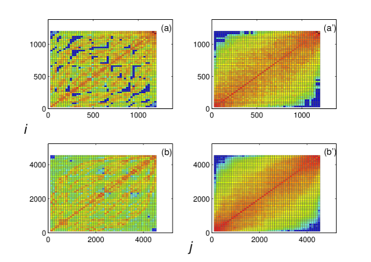
Let us denote the matrix of spin $I$ states of the nuclear shell model Hamiltonian $H$ by $H^{(I)}$, and the matrix elements of $H^{(I)}$ by $H_{ij}^{(I)}$, where $i$ and $j$ represent indices of basis states. In Fig. 1, we present two typical examples of distributions of the magnitude of $H_{ij}^{(I)}$, based on the $J^{\pi}=0^{+}$ and $J^{\pi}=2^{+}$ states of the ²⁴Mg nucleus. The color from blue to red corresponds to values from zero to large magnitudes. From panels (a-b) of Fig. 1, one sees that the values of $H_{ij}^{(I)}$ (panels (a-b) of Fig. 1) look ``random". However, if one sorts the diagonal matrix elements from the smaller to larger values, as in Refs. Shen2 , the values of $H_{ij}^{(I)}$ decrease rapidly and become zero if they are ``far" enough from the diagonal line, as shown in panels (a^′-b^′) of Fig. 1.

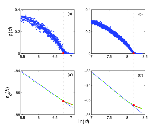
Let us investigate this behavior in another form. We study the probability for $H_{ij}^{(I)}$ to be non-zero (after sorting the diagonal matrix elements of $H_{ij}^{(I)}$), while moving away from the diagonal line, versus $d$, denoted by $\rho(d)=\frac{\sum{|{\rm sgn}(H_{i,i+d}^{(I)})|}}{D-d},$ $d=1,2,3,\cdots,D$. Here $d$ is the ``distance" of $H_{ij}^{(I)}$ from the diagonal line, and $D$ is the dimension of matrix $H_{ij}^{(I)}$ for spin $I$ states. As shown in Fig. 2(a) and (b) for the $I^{\pi}=0^{+}$ and $2^{+}$ states of the ²⁴Mg nucleus, $\rho(d)$ becomes zero at a critical value $d=d_{0}$; the value of ln$\,d_{0}$ equals 6.75 and 8.22, respectively.

An argument for the regular patterns described in Fig. 1 and Fig.2 (a) and (b) is as follows. With the diagonal matrix elements sorted from the smaller to larger values, one classifies configurations from the lowest to the largest in energy, roughly by particle-hole excitations. Configurations that come first are the lowest, and the states that come last are $n$-particle-$n$-hole excitations out of those low configurations. Because the shell-model Hamiltonian consists of one-body and two-body operators, one can not connect those configurations that are ``distant", e.g., the configurations with the lowest energy and $n$-particle-$n$-hole configurations with $n>2$. This explains the reason why all values of $H_{ij}^{(I)}$ become zero for $d\geq d_{0}$. Soon we shall find that the value of $d_{0}$ is very important in predicting the lowest eigenvalue of the matrix $H^{(I)}$.

Figure 1: (Color online) Magnitude of the matrix elements without (panels (a) and (b)) and with (panels (a^′) and (b^′)) sorting the diagonal matrix elements from the smaller to the larger. The color from blue to red corresponds to values from zero to large magnitudes. The results are based on $I^{\pi}=0^{+}$ (panels a and a^′) and $I^{\pi}=2^{+}$ (panels b and b^′) states of the ²⁴Mg nucleus, obtained by using the USD interactions. The magnitude of $H_{ij}^{(I)}$ without sorting the diagonal matrix elements (left hand side) are close to ``random", and those with sorting the diagonal matrix elements (right hand side) decrease rapidly as going farther from the diagonal line.

Figure 2:   (Color online)   Distribution for $H_{ij}^{(I)}$ to be non-zero, denoted by $\rho(d)$, and the lowest eigenvalues of $h$, denoted by $\epsilon_{d}(h)$. The results of (a,a^′) and (b,b^′) are obtained for the $J^{\pi}=0^{+}$ and $J^{\pi}=2^{+}$ states of ²⁴Mg, respectively. One sees that the values of $d$ where $\rho(d_{0})=0$ and where the $\epsilon_{d}(h)$-ln$\,d$ plots change the slope ($D_{0}$) coincide, i.e., $d_{0}=D_{0}$. We use the same scale in (a,a^′) or (b,b^′). The dotted lines are used to guide the eyes.

In Refs. V ; Yoshinaga1 ; Shen1 the lowest eigenvalue is presented in terms of ln$D$, where $D$ is the dimension of the matrix $H^{(I)}$. Although the formulas of the lowest eigenvalues presented in Refs. V ; Yoshinaga1 ; Shen1 are applicable to the random ensemble average (not to individual sets of interactions parameters), one naturally asks whether or not certain plots of the lowest eigenvalue versus the dimension could be useful in evaluating the lowest eigenvalue of realistic systems studied in this paper. Let us sort the diagonal matrix elements from the smaller to the larger, as in Refs. Shen2 . Then we truncate artificially the matrix $H^{(I)}$ and obtain a ``sub-matrix" $h$ with dimension $d$ ($d<D$), and $h_{ij}=H_{ij}^{(I)}$ ($i,j=1,2,\cdots,d$). We diagonalize $h$ and obtain the lowest eigenvalue $\epsilon_{d}$ of the matrix $h$, and plot $\epsilon_{d}$ versus ln$\,d$. In Fig. 2(a^′-b^′) we present the $\epsilon_{d}$-ln$\,d$ plots for the $I^{\pi}=0^{+}$ and $2^{+}$ states of the ²⁴Mg nucleus. One sees that $\epsilon_{d}$ decreases linearly with ln$\,d$ when $d$ is smaller than a critical dimension $d=D_{0}$, and decrease again linearly with ln$\,d$ but with a smaller slope. Apparently, the value of $D_{0}$ and the slopes for both $d<D_{0}$ and $d>D_{0}$ suffice for the evaluation of the lowest eigenvalue of $H_{ij}^{(I)}$.

In Fig. 2 one sees that the values of $d_{0}$ where $\rho(d_{0})=0$ in Fig. 2(a) and (b) coincide with $D_{0}$ in Fig. 2(a^′) and (b^′), respectively. Panels (a,b) are based on the same matrices as (a^′,b^′), respectively. For convenience, we use the same scale in panels (a,a^′) and (b,b^′), and plot two dotted lines to guide the eyes in order to see such coincidence. From Fig. 2 one also sees that the slope for $d>d_{0}$ (denoted by $k^{\prime}$) is smaller than that for $d<d_{0}$ (denoted by $k$).

An intuitive understanding of the facts that $d_{0}\simeq D_{0}$ and $k^{\prime}<k$ is given as follows. Because $H_{ij}^{(I)}$ are zero when $d>d_{0}$ (i.e., $\rho(d_{0})=0$ for $i,j>d_{0}$), there is no contribution to the lowest eigenvalue from these matrix elements. On the other hand, some of matrix elements $H_{ij}^{(I)}$ and $H_{ji}^{(I)}$, with $0<i<D-d_{0}$ and $j>D-d_{0}$, are non-zero (see Fig. 1(a^′) and (b^′)), lowering down the smallest eigenvalue of the $h$ matrix. The slope of the $\epsilon_{d}$-ln$\,d$ plot therefore changes at $d=d_{0}$ and becomes smaller for $d>d_{0}$ than that of $h$ for $d<d_{0}$.

Figure 3:   (Color online)   Distribution for ln($D_{0}$)/ln($d_{0}$) and $k^{\prime}/k$ for two hundred $H^{(I)}$ matrices for a number of nuclei in the sd shell, the dimension $D$ of which goes from 500 to 10000, by taking the USD interactions. One sees that ln($D_{0}$)/ln($d_{0})\simeq 1$, and that $k^{\prime}\sim\frac{2}{5}k$ with considerable fluctuations. In this paper we assume that ln($D_{0}$)/ln($d_{0}$)=1 and $k^{\prime}=\frac{2}{5}k$ when we predict the lowest eigenvalue of $H^{(I)}$, for simplicity.

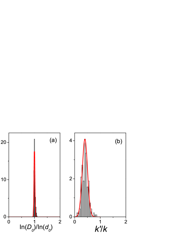
In Fig. 3 we present our results of ln($D_{0}$)/ln($d_{0}$) and $k^{\prime}/k$, based on 200 examples of $H^{(I)}$ for a number of $sd$ shell nuclei by using the USD interactions. One sees that ln($D_{0}$)/ln($d_{0}$) are very close to 1.0 and that $k^{\prime}\simeq\frac{2}{5}k$ with fluctuations. For simplicity we assume that ln($D_{0}$)/ln($d_{0}$)=1 and $k^{\prime}=\frac{2}{5}k$ for all cases throughout this paper.

Making use of these regularities, we obtain a new and simple formula to evaluate the lowest eigenvalue of the matrix $H^{(I)}$:

$$E_{\rm min}^{(I)} = \frac{2k}{5}{\rm ln}D+\left(k{\rm ln}d_{0}+b-\frac{2k}{5}{\rm ln}d_{0}\right)$$ (1)

$$= \frac{2k}{5}{\rm ln}(D)+\frac{3k}{5}{\rm ln}(d_{0})+b,$$

where $k$ and $b$ are the slope and intercept of the $\epsilon_{d}$-ln$\,d$ plot for $d<d_{0}$; $d_{0}$ is determined by $\rho(d_{0})=0$, and $D$ is the number of spin $I$ states. Because the $\epsilon_{d}$-ln$\,d$ plot shows a nice linearity (see Fig. 2(a^′,b^′)), we extract the values of $k$ and $b$ based on sub-matrices $h$ of $H^{(I)}$ with $d\leq D/10$ for all cases.

In Fig. 4 we present a comparison of the lowest states of spin $I$ predicted by the above Eq. (1), and those obtained by the linear correlation (i.e., Eq. (3) of Ref. Shen2 ), with those calculated by diagonalizing $H^{(I)}$ ($I=0,2,4,6,8$) for two nuclei, ²⁴Mg and ²⁸Si. One sees the remarkable agreement between the exact eigenvalues (the column ``exact") and our predicted ones (``pred1"), and substantial improvements achieved by Eq. (1) in comparison with Eq. (3) of Ref. Shen2 (``pred2" in Fig. 4). Without going into details, we mention that the overall root-mean-squared deviation ${\cal E}$ for the two-hundred cases we checked in Fig. 3 (defined by ${\cal E}=\sum_{i}^{N}\sqrt{(E^{\rm exact}_{i}-E^{\rm pred})^{2}/N}$, where $N$ is the number of examples that we checked and here $N=200$) is $0.38$ MeV, assuming that $d_{0}=D_{0}$, $k^{\prime}=\frac{2}{5}k$ for all examples.

Figure 4:   (Color online)   Comparison of low-lying levels obtained by exact diagonalization (denoted by ``exact") and those predicted by using Eq. (1) (denoted by ``pred1") and the linear correlation formula suggested in Ref. Shen2 (denoted by ``pred2") for the ²⁴Mg nucleus in panel (a), and the ²⁸Si nucleus in panel (b). The results are obtained by using the Yukawa-type interaction of Refs. Arima ; Takada4 . One sees substantial improvement of predictions for the lowest eigenvalues for each spin $I$ by using Eq. (1) of this paper.

Here we give a brief discussion of formulas in Refs. V ; Papenbrock1 ; Yoshinaga1 ; Shen1 ; Shen2 and the formula proposed in this paper. Ref. Papenbrock1 reported a correlation between the lowest eigenvalue and the spectral width $\sigma$ of the spin $I$ states. Ref. V suggested a simple formula $E_{\rm min}^{(I)}=\bar{E}_{I}-\sqrt{{\rm ln}D/{\rm ln}2}~{}\sigma$, where $\bar{E}_{I}$ is the average energy of spin $I$ states. Ref. Yoshinaga1 suggested a formula $E_{\rm min}^{(I)}=\bar{E}_{I}-\sqrt{a{\rm ln}D+b}~{}\sigma$ (similar to Ref. V ), with $a\simeq 1.00$ and $b\simeq 0.40$. Ref. Shen2 refined the results of Ref. Yoshinaga1 by including the third moment analytically, with an additional factor $\left(1-\frac{\sqrt{\pi}}{6\sqrt{2}}\left(\frac{\sigma_{3}}{\sigma}\right)^{3}\right)$ multiplied in the second term of the formula in Ref. Yoshinaga1 . Here $\sigma_{3}$ is the third moment of the eigenvalues. These formulas are applicable to the random Hamiltonians statistically (i.e., the ensemble average), not to the individual Hamiltonians such as for realistic systems. In Refs. Shen2 , the formula by using the linear correlation between the eigenvalues and diagonal matrix elements is applicable to individual sets of parameters and works well for medium eigenvalues, but it does not work very well for the lowest (or the largest) eigenvalues. The formula proposed in this paper is found to predict remarkably well the lowest eigenvalues of the nuclear shell model Hamiltonian, as shown in Fig. 4. We should also add that there are many other efforts towards overcoming the limitation of dimension in diagonalizing large matrices, see refs. other-1 ; other-2 ; other-3 ; other-4 .

To summarize, in this paper we first investigated the distribution of non-zero off-diagonal matrix elements of the nuclear shell model Hamiltonian. We demonstrated that the non-zero off-diagonal matrix elements exhibit regular patterns, if one sorts the diagonal matrix elements from the smaller to larger values; without sorting the diagonal matrix elements, the off-diagonal matrix elements look random. Almost all matrix elements becomes zero, if the matrix elements are ``distant" enough from the diagonal line, after sorting the diagonal matrix elements.

A very simple formula of the lowest eigenvalue for the shell model Hamiltonian matrix $H^{(I)}$ is proposed, based on the regular patterns of the $\rho(d)$ and $\epsilon_{d}$-ln$\,d$ plots for sub-matrices $h$. There exists a ``critical" dimension, $D_{0}$, at which the slope of the $\epsilon_{d}$-ln$\,d$ plot changes. The slope for $d>D_{0}$ is empirically found to be equal to 2/5 of that for $d<D_{0}$ with fluctuations. The value of $D_{0}$ is found to be equal to $d_{0}$ which can be obtained easily by using $\rho(d_{0})=0$. Here $\rho(d)$ represents the probability for $H_{ij}$ to be non-zero while moving away from the diagonal line.

The overall root-mean-squared deviation for two-hundred shell model Hamiltonians of nuclei in the $sd$ shell is $0.38$ MeV (the relative deviation is about $0.003$), assuming that $d_{0}=D_{0}$ and $k^{\prime}=\frac{2}{5}k$, with $k$ and $b$ obtained from the sub-matrices $h$ of $H^{(I)}$. The dimension of $h$ is much smaller than $D$, and here we take $d\leq D/10$. This demonstrates that our predicted results of the lowest eigenvalue based on our new formula are in very good agreement with the exact values, even if one treats much smaller ``sub-matrices" of $H^{(I)}$. We therefore expect that our new formula has significance for future theoretical studies of nuclear structure. It will be also interesting to investigate whether or not other low-lying states have similar features.

What has not been yet understood at a microscopic level is why the $\epsilon_{d}$-ln$\,d$ plot exhibits a remarkable linearity. Further consideration of these issues is warranted in future studies.

Acknowledgements: We thank the National Natural Science Foundation of China for supporting this work under grant 10975096. This work is also supported partly by Chinese Major State Basic Research Developing Program under Grant 2007CB815000.

References

- (1) K. F. Ratcliff, Phys. Rev. C 3. 117 (1971).
- (2) F. J. Margetan, A. Klar, and J. P. Vary, Phys. Rev. C 27. 852 (1983).
- (3) V. Velázquez and A. P. Zuker, Phys. Rev. Lett. 88, 072502 (2002).
- (4) T. Papenbrock and H. A. Weidenmueller, Phys. Rev. Lett 93, 132503 (2004); T. Papenbrock and H. A. Weidenmueller, Phys. Rev. C 73, 014311 (2006);
- (5) T. Papenbrock and H. A. Weidenmueller, Rev. Mod. Phys. 79, 997 (2007); H. A. Weidenmueller and G. E. Mitchell, Rev. Mod. Phys. 81, 539 (2009).
- (6) N. Yoshinaga, A. Arima and Y. M. Zhao, Phys. Rev. C73, 017303 (2006).
- (7) J. J. Shen, Y. M. Zhao, A. Arima and N. Yoshinaga, Phys. Rev. C 77, 054312 (2008).
- (8) J. J. Shen, A. Arima, Y. M. Zhao and N. Yoshinaga, Phys. Rev. C 78, 044305 (2008); N. Yoshinaga, A. Arima, J. J. Shen and Y. M. Zhao, Phys. Rev. C 79, 017301 (2009).
- (9) ftp://ftp.kutl.kyushu-u.ac.jp/pub/takada/jjSMQ/.
- (10) S. Yasumoto, Yoshifumi R. Shimizu and K. Takada, Prog. Theor. Phys. 116, 107 (2006).
- (11) K. Takada, M. Sato and S. Yasumoto, Prog. Theor. Phys. 104, 173 (2000); S. Yasumoto, Yoshifumi R. Shimizu and K. Takada, Prog. Theor. Phys. 110, 1037 (2000).
- (12) B. H. Wildenthal, Prog. Part. Nucl. Phys. 11, 5 (1984); B. A. Brown and B. H. Wildenthal, Annu. Rev. Nucl. Part. Sci. 38, 29 (1988).
- (13) T.Inoue, T.Sebe, H. Hasegawa and A.Arima, Nucl. Phys. 59, 1 (1964); Y. Akiyama, A. Arima and T.Sebe, Nucl. Phys. A138, 273 (1969).
- (14) S. E. Koonin, D. J. Dean, and K. Langanke, Phys. Rep. 577, 1 (1996); T. Otsuka, M. Honma, T. Mizusaki, N. Shimizu, and Y. Utsuno, Prog. Part. Nucl. Phys. 47, 319 (2001).
- (15) M. Horoi, A. Volya, and V. Zelevinsky, Phys. Rev. Lett. 82, 2064 (1999); M. Horoi, B. A. Brown, and V. Zelevinsky, Phys. Rev. C 65, 027303 (2002); M. Horoi, B. A. Brown, and V. Zelevinsky, Phys. Rev. C 67, 0034303 (2003); M. Horoi, J. Kaiser, and V. Zelevinsky, Phys. Rev. C 67, 054309 (2003)
- (16) T. Mizusaki and M. Imada, Phys. Rev. C 67, 041301 (2003); T. Mizusaki, Phys. Rev. C 70, 044316 (2004).
- (17) T. Papenbrock, A. Juodagalvis, and D. J. Dean, Phys. Rev. C 69, 024312 (2004); W. G. Wang, Phys. Rev. E 63, 036215 (2001).