Third-Order Gas-Liquid Phase Transition and the Nature of Andrews Critical Point

Abstract.

The main objective of this article is to study the nature of the Andrews critical point in the gas-liquid transition in a physical-vapor transport (PVT) system. A dynamical model, consistent with the van der Waals equation near the Andrews critical point, is derived. With this model, we deduce two physical parameters, which interact exactly at the Andrews critical point, and which dictate the dynamic transition behavior near the Andrews critical point. In particular, it is shown that 1) the Andrews critical point is a switching point where the phase transition changes from the first order to the third order, 2) the gas-liquid co-existence curve can be extended beyond the Andrews critical point, and 3) the liquid-gas phase transition going beyond Andrews point is of the third order. This clearly explains why it is hard to observe the gas-liquid phase transition beyond the Andrews critical point. Furthermore, the analysis leads naturally the introduction of a general asymmetry principle of fluctuations and the preferred transition mechanism for a thermodynamic system.

1. Introduction

Phase transition is one of the central problems in nonlinear sciences. Many systems have different phases, and the most commonly encountered phases are gas, liquid and solid phases. A natural system which possesses these three phases is the physical-vapor transport (PVT) system. As we know, a $PVT$ system is a system composed of one type of molecules, and the interaction between molecules is governed by the van der Waals law. The molecules generally have a repulsive core and a short-range attraction region outside the core. Such systems have a number of phases: gas, liquid and solid, and a solid can appear in a few phases. The most typical example of a $PVT$ system is water.

A $PT$-phase diagram of a typical $PVT$ system is schematically illustrated by Figure 1.1, where point $A$ is the triple point at which the gas, liquid, and solid phases can coexist. Point $C$ is the Andrews critical point at which the gas-liquid coexistence curve terminates [3, 4]. Classical view on the termination of the gas-liquid coexistence curve at the critical point amounts to saying that the system can go continuously from a gaseous state to a liquid state without ever meeting an observable phase transition, if we choose the right path.

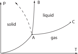
Figure 1.1. Coexistence curves of a typical $PVT$ system: $A$ is the triple point, $C$ is the critical point, and the dashed cure is a melting line with negative slope.

It is, however, still an open question why the Andrews critical point exists and what is the order of transition going beyond this critical point. In [1], a mathematical theory is derived to address this problem. In this article, we explore the physical implications of the mathematical theory derived in [1], give a theory on the nature of the Andrews critical point, and introduce the asymmetry principle of fluctuations and the preferred transition mechanism.

First, the modeling is based on 1) the Landau mean field theory, 2) a unified dynamic approach for equilibrium phase transitions, 3) the classical phase diagram in Figure 1.1, and c) the van der Waals equation. It is worth mentioning two important aspects of the model we derived. One is that the new model can be used to study liquid-solid and gas-solid transitions as well, by choosing different parameters. Second is the consistency of the model with the van der Waals equation. Namely, near the Andrews critical point $C$, the steady state equation of the homogeneous model (2.12) is exactly the van der Waals equation. This consistency gives a good validation of the mean field model. In addition, the dynamic approach leading to the model provides much richer information. For example, the model (2.7) can be used to study the heterogeneity of the system.

Second, with the dynamic model at our disposal, we introduce two new physical parameters $\lambda=\lambda(T,p)$ and $a_{2}=a_{2}(T,p)$, where the temperature $T$ and the pressure $p$ are control parameters. These two physical parameters determine the phase transition behavior near the Andrews point and provide the key ingredient to characterize the nature of the Andrews point.

It is remarkable that these two parameters reproduce the location of the Andrews critical point $C$, which is the same as derived by van der Waals in his classical work, although the method we use is the dynamic approach based on the Landau mean field theory, different from the one used by van der Waals. Coincidentally, these two parameters are the second and third-order derivatives of the Gibbs energy at the equilibrium state $\rho_{0}$; see (3.3).

Third, the two parameters $\lambda$ and $a_{2}$ correspond to two-curves in the $pT$-phase plane, and interact exactly at the Andrews critical point $C$. Then with the dynamic transition theory developed recently by the authors, we deduce a theory on the Andrews critical point $C$: 1) the critical point is a switching point where the phase transition changes from the first order with latent heat to the third order, and 2) the gas-liquid phase transition beyond the Andrews critical point is of the third order. This explains why it is hard to observe the phase liquid-gas transition beyond the Andrews point, and clearly

Fourth, physical intuition and the theory lead us to introduce asymmetry principle of fluctuations, and the preferred transition mechanism.

2. A Dynamic Model for Gas-Liquid Transition

The classical and the simplest equation of state which can exhibit many of the essential features of the gas-liquid phase transition is the van der Waals equation:

(2.1) $$\left(p+\frac{a}{v^{2}}\right)(v-b)=RT,$$

where $v$ is the molar volume, $p$ is the pressure, $T$ is the temperature, $R$ is the universal gas constant, $b$ is the revised constant of inherent volume, and $a$ is the revised constant of attractive force between molecules. If we adopt the molar density $\rho=1/v$ to replace $v$ in (2.1), then the van der Waals equation becomes

(2.2) $$-(bp+RT)\rho+a\rho^{2}-ab\rho^{3}+p=0.$$

Now, we shall apply thermodynamic potentials to investigate the gas-liquid phase transitions in $PVT$ systems, and we shall see later that the van der Waals equation can be derived as a Euler-Langrange equation for the minimizers of the Gibbs free energy for $PVT$ systems at gaseous states.

Consider an isothermal-isopiestic process. The thermodynamic potential is taken to be the Gibbs free energy. In this case, the order parameters are the molar density $\rho$ and the entropy density $S$, and the control parameters are the pressure $p$ and temperature $T$. The general form of the Gibbs free energy for $PVT$ systems is given as

(2.3) $$G(\rho,S,T,p)=\int_{\Omega}\Big{[}\frac{\mu_{1}}{2}|\nabla\rho|^{2}+\frac{\mu_{2}}{2}|\nabla S|^{2}+g(\rho,S,T,p)-ST-\alpha(\rho,T,p)p\Big{]}dx,$$

where $g$ and $\alpha$ are differentiable with respect to $\rho$ and $S$, $\Omega\subset\mathbb{R}^{3}$ is the container, and $\alpha p$ is the mechanical coupling term in the Gibbs free energy, which can be expressed by

(2.4) $$\alpha(\rho,T,p)p=\rho p-\frac{1}{2}b\rho^{2}p,$$

where $b=b(T,p)$ depends continuously on $T$ and $p$. In fact, this mechanical coupling term should be $p$. In view of the van der Waals equation  (2.2) and the mathematical analysis based on the new dynamical transition theory, phenomenologically we need to adjust the term by adding a coefficient $\alpha$, leading to (2.4) as the first two terms in the Taylor expansion. Although the van der Waals equation works for gaseous sates only, by choosing the dependence of the coefficient $b$ on the temperature and the pressure, the energy applies to the liquid and solid states as well. This is a very subtle term from the physical point of view to derive a feasible free energy.

Based on both the physical and mathematical considerations, we take the Taylor expansion of $g(\rho,S,T,p)$ on $\rho$ and $S$ as follows

(2.5) $$g=\frac{1}{2}\alpha_{1}\rho^{2}+\frac{1}{2}\beta_{1}S^{2}+\beta_{2}S\rho^{2}-\frac{1}{3}\alpha_{2}\rho^{3}+\frac{1}{4}\alpha_{3}\rho^{4},$$

where $\alpha_{i}$ $(1\leq i\leq 3)$, $\beta_{1}$ and $\beta_{2}$ depend continuously on $T$ and $p$, and

(2.6) $$\beta_{1}=\beta_{1}(T,p)>0,\qquad\alpha_{i}=\alpha_{i}(T,p)>0\quad i=2,3.$$

In a $PVT$ system, the order parameter is $u=(\rho,S)$,

$$\rho=\rho_{1}-\rho_{0},\ \ \ \ S=S_{1}-S_{0},$$

where $\rho_{i}$ and $S_{i}$ $(i=0,1)$ represent the density and entropy, $\rho_{0},S_{0}$ are reference points near the coexistence curve of gas and liquid states. Hence the conjugate variables of $\rho$ and $S$ are the pressure $p$ and the temperature $T$. Thus, by the le Châtlier principle, we derive from (2.3)-(2.5) the following dynamic model for a $PVT$ system:

(2.7) $$\left.\begin{aligned} &\frac{\partial\rho}{\partial t}=\mu_{1}\Delta\rho-(\alpha_{1}+bp)\rho+\alpha_{2}\rho^{2}-\alpha_{3}\rho^{3}-2\beta_{2}\rho S+p,\\ &\frac{\partial S}{\partial t}=\mu_{2}\Delta S-\beta_{1}S-\beta_{2}\rho^{2}+T.\end{aligned}\right.$$

A physically meaningful boundary condition for the system is the Neumann boundary condition:

(2.8) $$\frac{\partial\rho}{\partial n}=0,\ \ \ \ \frac{\partial S}{\partial n}=0\qquad\text{ on }\partial\Omega.$$

An important special case for $PVT$ systems is that the pressure and temperature functions are homogeneous in $\Omega$. Thus we can assume that $\rho$ and $S$ are independent of $x\in\Omega$, and the free energy (2.3) with (2.4) and (2.5) can be expressed as

(2.9) $$G(\rho,S,T,p)=\frac{\alpha_{1}}{2}\rho^{2}+\frac{\beta_{1}}{2}S^{2}+\beta_{2}S\rho^{2}-\frac{\alpha_{2}}{3}\rho^{3}+\frac{\alpha_{3}}{4}\rho^{4}+\frac{b\rho^{2}p}{2}-\rho p-ST.$$

From (2.9) we get the dynamical equations as

(2.10) $$\left.\begin{aligned} &\frac{d\rho}{dt}=-(\alpha_{1}+bp)\rho+\alpha_{2}\rho^{2}-\alpha_{3}\rho^{3}-2\beta_{2}S\rho+p,\\ &\frac{dS}{dt}=-\beta_{1}S-\beta_{2}\rho^{2}+T.\end{aligned}\right.$$

Because $\beta_{1}>0$ for all $T$ and $p$, we can replace the second equation of (2.10) by

(2.11) $$S=\beta^{-1}_{1}(T-\beta_{2}\rho^{2}).$$

Then, (2.10) are equivalent to the following equation

(2.12) $$\frac{d\rho}{dt}=-(\alpha_{1}+bp+2\beta^{-1}_{1}\beta_{2}T)\rho+\alpha_{2}\rho^{2}-(\alpha_{3}-2\beta^{2}_{2}\beta^{-1}_{1})\rho^{3}+p.$$

It is clear that if $\alpha_{1}=0,2\beta^{-1}_{1}\beta_{2}=R,\alpha_{2}=a,(\alpha_{3}-2\beta^{2}_{2}\beta^{-1}_{1})=ab$, then the steady state equation of (2.12) is referred to the van der Waals equation.

We remark that(2.12) can be considered as the dynamic version of the van der Waals equation, although we used the Landau mean field theory together with the le Châtlier principle. The approach provides a much richer information. For example, the model (2.7) can be used to study the heterogeneity of the system. In addition, the model here can be used to study liquid-solid and gas-solid transitions as well, by choosing different parameters.

3. Two New Physical Parameters and the Andrews Critical Point

In this section we use (2.12) to derive two new physical parameters, which dictates the dynamic transition behavior near the Andrews critical points.

Let $\rho_{0}$ be a steady state solution of (2.12) near the Andrews point $C=(T_{c},p_{c})$. We take the transformation

$$\rho=\rho_{0}+\rho^{\prime}.$$

Then equation (2.12) becomes (drop the prime)

(3.1) $$\frac{d\rho}{dt}=\lambda\rho+a_{2}\rho^{2}-ab\rho^{3}.$$

where

(3.2) $$\lambda=2a\rho_{0}-3ab\rho^{2}_{0}-\alpha_{1}-bp-RT,$$

$$a_{2}=a(1-3b\rho_{0}).$$

where $\alpha_{1}$ is close to zero. Here we emphasize that $\rho_{0}$ and $(\lambda,a_{2})$ are all functions of the control parameters $(T,p)$.

These are two important physical parameters, which are used to fully characterize the dynamic behavior of gas-liquid transition near the Andrews point. In fact, from the derivation of the model, we obtain immediately the following physical meaning of these two parameters:

(3.3) $$\lambda(T,p)=\frac{d^{2}G}{d\rho^{2}}\big{|}_{\rho=\rho_{0}},\qquad a_{2}(T,p)=\frac{1}{2}\frac{d^{3}G}{d\rho^{3}}\big{|}_{\rho=\rho_{0}},$$

where $\rho_{0}=\rho_{0}(T,p)$ is the equilibrium state.

In the $PT$-plane, near the Andrews point $C=(T_{c},p_{c})$, the critical parameter equation

$$\lambda=\lambda(T,p)=0\qquad\text{in}\ \ \ \ |T-T_{c}|<\delta,\ \ \ \ |p-p_{c}|<\delta$$

for some $\delta>0$, defines a continuous function $T=\phi(p)$, such that

(3.4) $$\lambda\left\{\begin{aligned} &<0&&\text{ if }T>\phi(p),\\ &=0&&\text{ if }T=\phi(p),\\ &>0&&\text{ if }T<\phi(p).\end{aligned}\right.$$

Equivalently, this is called the principle of exchange of stabilities, which, as we have shown in [1], is the necessary and sufficient condition for the gas-liquid phase transition.

One important component of our theory is that the Andrews critical point is determined by the system of equations

(3.5) $$\lambda=0,$$

$$a_{2}=0,$$

$$-(bp+RT)\rho_{0}+a\rho_{0}^{2}-ab\rho_{0}^{3}+p=0.$$

Here the first equation is the critical parameter equation, the second equation, as we shall see below, determines the switching point where the phase transition switches types, and the last equation is the van der Waals equation, which is also the steady state equation of the dynamic model.

Then by a direct computation, it is easy to see that the critical point $C$ is given by

(3.6) $$(\rho_{c},T_{c},p_{c})=\left(\frac{1}{3b},\frac{a}{27b^{2}},\frac{8a}{27bR}\right).$$

This is in agreement with the classical work by van der Waals. Here we obtain the Andrews point using a dynamic approach.

4. Theory of the Andrews Critical Point

We now explain the gas-liquid transition near the Andrews critical point $C$.

First, we have shown in (3.6) that at the equilibrium point $\rho_{0}$, the two curves given by $\lambda(p,T)=0$ and $a_{2}(p,T)=0$ interact exactly at the critical point $C$ as shown in Figure 4.1, and the curve segment $AB$ of $\lambda=0$ is divided into two parts $AC$ and $CB$ by the point $C$ such that

$$a_{2}(T,p)>0\ \ \ \ \text{for}\ \ \ \ (T,p)\in AC,$$

$$a_{2}(T,p)<0\ \ \ \ \text{for}\ \ \ \ (T,p)\in CB.$$

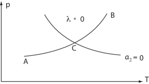
Figure 4.1. The point $C=(T_{c},p_{c})$ is the Andrews critical point.

Here the curve $AC$ is the classical gas-liquid co-existence curve.

Second, on the curve $AC$, excluding the critical point $C$, $a_{2}(T,p)>0$. The phase transition of the system is a mixed type if we take a pass crossing the $AC$; see Figure 4.2. In Figure 4.2, $\rho$ is the deviation from the basic gaseous state $\rho_{0}$. We now consider different states given in Figure 4.2(a):

1. 

   

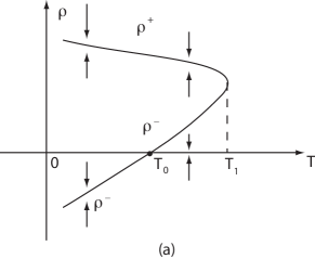
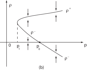
   Figure 4.2. Type-III (mixed) transition for $a_{2}>0$: (a) Phase diagram for fixed pressure, and (b) phase diagram for fixed temperature.

2. For $T>T_{1}$, the gaseous state $\rho_{0}$, corresponding to $\rho=0$ in the figure, is stable. This is the only stable physical state in this temperature range, and the system is in the gaseous state.

3. For $T_{0}<T<T_{1}$, there are two metastable states given by gaseous phase $\rho_{0}$ and the liquid phase $\rho_{0}+\rho^{+}$.

4. For $T<T_{0}$, there are three states: the unstable basic gaseous state $\rho_{0}$, and the two metastable states: $\rho_{0}+\rho^{-}$ and $\rho_{0}+\rho^{+}$. One important component of our theory is that the only physical phase here is the liquid phase represented by metastable state: $\rho_{0}+\rho^{+}$. Although, mathematically speaking, the gaseous state $\rho_{0}+\rho^{-}$ is also metastable, it does not appear in nature. The only possible explanation for this exclusion is the asymmetry principle of fluctuations, to be further explored in the next section.

5. Hence we have shown that as we lower the temperature, the system undergoes a first order transition from a gaseous state to a liquid state with an abrupt change in density. In fact, there is an energy gap between the gaseous and liquid states:

   $$\Delta E=G(\rho_{0}+\rho^{+})-G(\rho_{0})\sim-\frac{\lambda}{4}(\rho^{+})^{2}-\frac{a_{2}}{12}(\rho^{+})^{3}<0\ \ \ \ \text{for }\ T<T_{1};$$

   see [1]. This energy gap $|\Delta E|$ stands for a latent heat, and $\Delta E<0$ shows that the transition from a gaseous state to a liquid state is an isothermal exothermal process, and from a liquid state to gaseous state is an isothermal endothermal process.

Third, at the critical point $C$, we have $a_{2}=0$. Then the dynamic transition is as shown in Figure 4.3; see [1] for the detailed mathematical analysis leading to this phase diagram:

1. As in the previous case, for $T>T_{0}$, the only physical state is given by the gaseous phase $\rho_{0}$, corresponding to zero deviation shown in the figure.

2. As the temperature $T$ is lowered crossing $T_{0}$, the gaseous state losses its stability, leading to two metastable states: one is the liquid phase $\rho_{0}+\rho^{+}$, and the other is the gaseous phase $\rho_{0}+\rho^{-}$. Again, the gaseous phase $\rho_{0}+\rho^{-}$ does not appear, and the asymmetry principle of fluctuations is valid in this situation as well.

3. The phase transition here is of the second order, as the energy is continuous at $T_{0}$. In fact, the energy for the transition liquid state is given by

   $$G(\rho_{0}+\rho^{+})=G(\rho_{0})-\frac{\alpha^{2}}{4a_{3}}(T-T_{c})^{2}\ \ \ \ \text{for}\ T<T_{c},$$

   for some $\alpha>0$. Hence the difference of the heat capacity at $T=T_{c}$ is

   $$\Delta C=-T_{c}\frac{\partial^{2}}{\partial T^{2}}\left(G(\Phi^{+}(T_{c}^{+}))-G(\rho_{0})\right)=\frac{\alpha^{2}}{2a_{3}}T_{c}>0.$$

   Namely the heat capacity has a finite jump at $T=T_{c}$, therefore the transition at $T=T_{c}$ is of the second order.

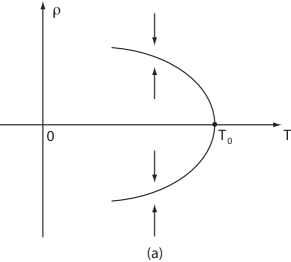
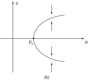
Figure 4.3. Continuous transition for the case where $a_{2}=0.$

Fourth, on the curve $BC$, $a_{2}(T,p)<0$, and the phase transition diagram is given by Figure 4.4:

1. For $T>T_{1}$, the system is in the gaseous phase, which is stable.

2. For $T_{0}<T<T_{1}$, there are two metastable gaseous states given by $\rho_{0}$ and $\rho_{0}+\rho^{-}$. As before, although it is metastable, the gaseous state $\rho_{0}+\rho^{-}$ does not appear.

3. For $T<T_{0}$, the gaseous phase $\rho_{0}$ losses its stability, and the system undergoes a dynamic transition to the metastable liquid state $\rho_{0}+\rho^{+}$. Mathematically, the gaseous state $\rho_{0}+\rho^{-}$ is also metastable. However, it does not appear either, due to the asymmetry principle of fluctuations.

4. The dynamic transition in this case is of the third order. In fact, we have

   $$G(\rho_{0}+\rho^{+})=G(\rho_{0}(T))-\frac{\alpha^{3}}{6|a_{2}|^{2}}(T_{0}-T)^{3}+o(|T_{0}-T|^{3})\text{ for }T<T_{0}.$$

   Namely, the free energy is continuously differentiable up to the second order at $T=T_{0}$, and the transition is of the third order. It implies that as $(T_{0},p_{0})\in CB$ the third-order transition at $(T_{0},p_{0})$ can not be observed by physical experiments.

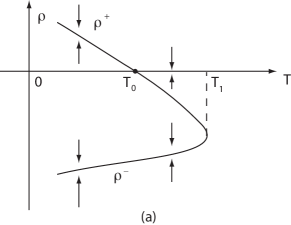
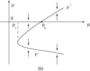
Figure 4.4. Type-III (mixed) transition for $a_{2}<0$.

In summary, we have obtained a precise characterization of the phase transition behavior near the Andrews point, and have derived precisely the nature of the Andrews critical point. In particular, we have shown the following:

1. The transition is first order before the critical point, second-order at the critical point, and third order after the critical point.

2. The curve $\lambda(T,p)=0$ always defines the gas-liquid co-existence curve in both sides of the critical point $C$. We note that in the classical theory, the co-existence curve terminates at the critical point, and with our theory, we are able to determine the gas-liquid transition behavior and the co-existence curve beyond the critical point.

5. Asymmetry Principle of Fluctuations and the Preferred Transition Mechanism

We have shown in the last section that in all three cases (both sides of the critical point and at the critical point), the metastable state $\rho_{0}+\rho^{-}$ does not appear. Hence the only possible physical explanation is the asymmetry of the fluctuations. In fact, for the ferromagnetic systems we also see this asymmetry of fluctuations [2]. This observation leads to the following important principle:

Physical Principle (Asymmetry of Fluctuations). The symmetry of fluctuations for general thermodynamic systems may not be universally true. In other words, in some systems with multi-equilibrium metastable states, the fluctuations near a critical point occur only in one basin of attraction of some equilibrium states, which are the ones that can be physically observed.

An alternate explanation of this principle is related to phase transitions in certain preferred direction in a given thermodynamic system, which we call preferred transition mechanism. We conjecture that this mechanism is universal as well. Here we use this mechanism to explain the asymmetry principle of fluctuations in the gas-liquid transition, and, in return, to explain the meaning of the preferred transition mechanism.

In the gas-liquid transition as the temperature is lowered, the system prefers phase transitions to denser phase. This can be considered as one aspect of the preferred transition mechanism.

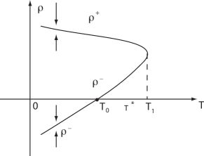
Figure 5.1. Preferred transition mechanism for $a_{2}>0$ with fixed pressure.

Another important aspect of the mechanism is the preferred transition at a critical point $T^{\ast}$ as shown in Figure 5.1, which is reproduced from Figure 4.2(a). This critical point is between $T_{0}$ and $T_{1}$, and for water under one atmospheric pressure, $T^{*}$ is 100 ^oC. For $T^{*}<T<T_{1}$, the liquid state state $\rho_{0}+\rho^{+}$ is called superheated liquid, and for $T_{0}<T<T^{*}$, the gaseous state $\rho_{0}$ is called supercooled gas. The preferred transition mechanism consists of the following:

1. As temperature decreases, the system is forced to undergo a first-order transition at $T=T^{*}$, from the gas state $\rho_{0}$ to the liquid state $\rho_{0}+\rho^{+}$.

2. As the temperature increases, the system is forced to undergo a first-order liquid $\rho_{0}+\rho^{+}$ to gas $\rho_{0}$ transition as the same critical point $T=T^{*}$.

3. The supercooled gas and superheated liquid can rarely occur. Physically, this is related to the hysteresis phenomena.

References

- [1] T. Ma and S. Wang, Dynamic phase transition theory in PVT systems, Indiana University Mathematics Journal, 57:6 (2008), pp. 2861–2889.
- [2] , Dynamic transitions for ferromagnetism, Journal of Mathematical Physics, 49:053506 (2008), pp. 1–18.
- [3] L. E. Reichl, A modern course in statistical physics, A Wiley-Interscience Publication, John Wiley & Sons Inc., New York, second ed., 1998.
- [4] H. E. Stanley, Introduction to Phase Transitions and Critical Phenomena, Oxford University Press, New York and Oxford, 1971.