Darknet-Based Inference of Internet Worm Temporal Characteristics

Abstract

Internet worm attacks pose a significant threat to network security and management. In this work, we coin the term Internet worm tomography as inferring the characteristics of Internet worms from the observations of Darknet or network telescopes that monitor a routable but unused IP address space. Under the framework of Internet worm tomography, we attempt to infer Internet worm temporal behaviors, i.e., the host infection time and the worm infection sequence, and thus pinpoint patient zero or initially infected hosts. Specifically, we introduce statistical estimation techniques and propose method of moments, maximum likelihood, and linear regression estimators. We show analytically and empirically that our proposed estimators can better infer worm temporal characteristics than a naive estimator that has been used in the previous work. We also demonstrate that our estimators can be applied to worms using different scanning strategies such as random scanning and localized scanning.

1 Introduction

Since Code Red and Nimda worms were released in 2001, epidemic-style attacks have caused severe damages. Internet worms can spread so rapidly that existing defense systems cannot respond until most vulnerable hosts have been infected. For example, on January 25th, 2003, the Slammer worm reached its maximum scanning rate of more than 55 million scans per second in about 3 minutes, and infected more than 90% of vulnerable machines within 10 minutes [1]. It cost over one billion US dollars in cleanup and economic damages. Therefore, worm attacks pose significant threats to the Internet and meanwhile present tremendous challenges to the research community.

To counteract these notorious plague-tide attacks, various detection and defense strategies have been studied in recent years. According to where the detectors are located, these strategies can generally be classified into three categories: source detection and defenses, detecting infected hosts in the local networks [2, 3, 4, 5]; middle detection and defenses, revealing the appearance of worms by analyzing the traffic going through routers [6, 7, 8]; and destination detection and defenses, monitoring unwanted traffic arriving at Darknet or network telescopes, a globally routable address space where no active services or servers reside [9, 10, 11, 12, 13]. There are two types of Darknet: active Darknet that responds to malicious scans to elicit the payloads of the attacks [11, 12], and passive Darknet that observes unwanted traffic passively [10, 13].

Different from source and middle detection and defenses, destination detection and defenses offer unique advantages in observing large-scale network explosive events such as distributed denial-of-service (DDoS) attacks [14] and Internet worms [15, 1, 16]. There is no legitimate reason for packets destined to Darknet. Hence, most of the traffic arriving at Darknet is malicious or unintended, including hostile reconnaissance scans, probe activities from active worms, DDoS backscatter, and packets from mis-configured hosts. Moreover, it has been shown that for a large-scale worm event, most of infected hosts, if not all, can be observed by the Darknet with a sufficiently large size [17].

In this work, we focus on the destination detection and defenses. Specifically, we study the problem of inferring the characteristics of Internet worms from Darknet observations. We refer to such a problem as Internet worm tomography, as illustrated in Fig.1. Most worms use scan-based methods to find vulnerable hosts and randomly generate target IP addresses. Thus, Darknet can observe partial scans from infected hosts. Together with the worm propagation model and the statistical model, Darknet observations can be used to detect worm appearance [18, 19, 20, 21] and infer worm characteristics (e.g., infection rate [22], number of infected hosts [17, 23], and worm infection sequence [24, 25, 26]). Internet worm tomography is named after network tomography, which infers the characteristics of the internal network (e.g., link loss rate, link delay, and topology) through the observations from end systems [27, 28]. Network tomography can be formulated as a linear inverse problem. Internet worm tomography, however, cannot be translated into the linear inverse problem due to the specific properties of worm propagation, and thus presents new challenges.

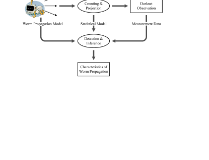
Figure 1: Internet worm tomography.

Under the framework of Internet worm tomography, researchers have studied worm temporal characteristics and have attempted to answer the following important questions:

• Host infection time: When exactly does a specific host get infected? This information is critical for the reconstruction of the worm infection sequence [25].

• Worm infection sequence: What is the order in which hosts are infected by worm propagation? Such an order can help identify patient zero or initially infected hosts [24].

The information of both the infection time and the infection sequence is important for defending against worms. First, the identification of patient zero or initially infected hosts and their infection times provide forensic clues for law enforcement against the attackers who wrote and spread the worm. Second, the knowledge of the infection sequence provides insights into how a worm spread across the Internet (e.g., characteristics on who infected whom) and how network defense systems were breached.

A simple estimator has been proposed in [25] to infer worm temporal behaviors. The estimator uses the observation time when an infected host scans the Darknet for the first time as the approximation of the host infection time to infer the worm infection sequence. Such a naive estimator, however, does not fully exploit all information obtained by the Darknet. Moreover, an attacker can design a smart worm that uses lower scanning rates for patient zero or initially infected hosts and higher scanning rates for other infected hosts. In this way, the smart worm would weaken the performance of the naive estimator.

The goal of this paper is to infer the Internet worm temporal characteristics accurately by exploiting Darknet observations and applying statistical estimation techniques. Our research work makes several contributions:

• We propose method of moments, maximum likelihood, and linear regression statistical estimators to infer the host infection time. We show analytically and empirically that the mean squared error of our proposed estimators can be almost half of that of the naive estimator in inferring the host infection time.

• We extend our proposed estimators to infer the worm infection sequence. Specifically, we formulate the problem of estimating the worm infection sequence as a detection problem and derive the probability of error detection for different estimators. We demonstrate analytically and empirically that our method performs much better than the algorithm proposed in [25].

• We show empirically that our estimators have a better performance in identifying patient zero or initially infected hosts of the smart worm than the naive estimator. We also demonstrate that our estimators can be applied to worms using different scanning strategies such as random scanning and localized scanning.

The remainder of this paper is organized as follows. Section 2 introduces estimators for inferring the host infection time. Section 3 presents our algorithms in estimating the worm infection sequence. Section 4 gives simulation results. Section 5 discusses the assumptions, the limitations, and the extensions of our estimators. Finally, Section 6 reviews related work, and Section 7 concludes the paper.

2 Estimating the Host Infection Time

We use Darknet observations to estimate when a host gets infected and use hit to denote the event that a worm scan hits the Darknet. As shown in Fig. 2, suppose that a certain host is infected at time $t_{0}$. The Darknet monitors a portion of the IPv4 address space and can observe some scans from this host and record hit times $t_{1},t_{2},\cdots,t_{n}$, where $n$ is the number of hit events from this host. The problem of estimating the host infection time can then be stated as follows: Given the Darknet observations $t_{1},t_{2},\cdots,t_{n}$, what is the best estimate of $t_{0}$?

To study this problem, we make the following assumptions: 1) There is no packet loss in the Internet. 2) An infected host uses its actual source IP address and does not apply IP spoofing, which is the case for TCP worms. 3) The scanning rate $s$ (i.e., the number of scans sent by an infected host per time unit) is time-invariant for an infected host, whereas the scanning rates of infected hosts can be different from each other. The last assumption comes from the observation that famous worms, such as Code Red, Nimda, Slammer, and Witty, do not apply any scanning rate variation mechanisms. An infected host always scans for vulnerable hosts at the maximum speed allowed by its computing resources and network conditions [29]. In Section 5, we will revisit and discuss these assumptions.

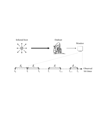
Figure 2: An illustration of Darknet observations.

Obviously, inferring $t_{0}$ from Darknet observations is affected by the Internet-worm scanning methods. In this paper, we focus on random scanning and localized scanning. However, if a scan from an infected host hits Darknet with a time-invariant probability, our estimation techniques are independent of worm-scanning methods. To analytically estimate the host infection time, we consider a discrete-time system. For random scanning (RS), a worm selects targets randomly and scans the entire IPv4 address space with $\Omega$ addresses (i.e., $\Omega=2^{32}$). We assume that Darknet monitors $\omega$ addresses. Thus, the probability for a scan to hit the Darknet is $\omega/\Omega$; and the probability of a hit event in the discrete-time system (i.e., the probability that Darknet observes at least one scan from the same infected host in a time unit) is

$$\mbox{Pr}_{\mbox{\tiny RS}}(\mbox{hit event})=1-\Big{(}1-\frac{\omega}{\Omega}\Big{)}^{s}.$$ (1)

Since $s$ is time-invariant for a given infected host, $\mbox{Pr}_{\mbox{\tiny RS}}(\mbox{hit event})$ is also time-invariant.

Localized scanning (LS) preferentially searches for vulnerable hosts in the “local” address space [30]. For simplicity, in this paper we only consider the $/l$ LS: $p_{a}(0\leq p_{a}<1)$ of the time, a “local” address with the same first $l$ bits as the attacking host is chosen as the target; $1-p_{a}$ of the time, a random address is chosen. We consider a centralized Darknet that occupies a continuous address space and monitors $\omega$ addresses. Moreover, we assume that the Darknet is contained in a $/l$ prefix with no vulnerable hosts. For example, network telescopes used by CAIDA are such a centralized Darknet and contain a $/8$ subnet. Since no infected hosts exist in the $/l$ subnet where the Darknet resides, the probability for a worm scan to hit the Darknet is $(1-p_{a})\cdot\omega/\Omega$. Therefore, the probability of a hit event in the discrete-time system is

$$\mbox{Pr}_{\mbox{\tiny LS}}(\mbox{hit event})=1-\Big{(}1-(1-p_{a})\cdot\frac{\omega}{\Omega}\Big{)}^{s},$$ (2)

which is time-invariant. Since $\mbox{Pr}_{\mbox{\tiny RS}}(\mbox{hit event})$ has a similar form as $\mbox{Pr}_{\mbox{\tiny LS}}(\mbox{hit event})$ and is the special case of $\mbox{Pr}_{\mbox{\tiny LS}}(\mbox{hit event})$ when $p_{a}$ = 0, we use $p$ ($0<p<1$) to denote the hit probability in general for both cases to simplify our discussion.

TABLE I: Notations used in this paper.

  Notations                        Definition $\Omega$ Size of the scanning space ($\Omega=2^{32}$) $\omega$ Size of the Darknet $s$ Scanning rate (scans/time unit) $\sigma$ Standard deviation of the scanning rate $p_{a}$ Probability that an address with the same first $l$ bits as the attacking host is chosen by LS $p$ Probability that at least one scan from the same infected host hits the Darknet in a time unit $t_{0}$ Host infection time $\hat{t}_{0}$ Estimated host infection time $t_{i}$ Discrete time tick when the infected host hits the Darknet for the $i$-th time $(i\geq 1)$ $\delta_{i}$ Time interval between two consecutive hits of the Darknet ($\delta_{i}=t_{i+1}-t_{i}$, $i\geq 1$) $n$ Number of hit events observed at the Darknet for an infected host $\mu$ Mean of $\delta$ $\hat{\mu}$ Estimation of $\mu$ $D$ Sequence distance $S_{i}$ Worm infection sequence $\hat{S_{i}}$ Estimated worm infection sequence $N$ Length of the worm infection sequence considered for evaluation  

Denote $\delta_{0}$ as the time interval between when a host gets infected and when Darknet observes the first scan from this host, i.e., $\delta_{0}=t_{1}-t_{0}$, as shown in Fig. 2. Denote $\delta_{i}$ as the time interval between $i$-th hit and $(i+1)$-th hit on Darknet, i.e., $\delta_{i}=t_{i+1}-t_{i}$, $i\geq 1$. Thus, $\delta_{0},\delta_{1},\cdots,\delta_{n-1}$ are independent and identically distributed (i.i.d.) and follow a geometric distribution with parameter $p$, i.e.,

$$\mbox{Pr}(\delta=k)=p\cdot(1-p)^{k-1},\ k=1,2,3,\cdots,$$ (3)

$$\mbox{E}(\delta)={1\over p}=\mu,\ \ \ \ \ \mbox{Var}(\delta)=\frac{1-p}{p^{2}}.$$ (4)

Denote $\mu$ as the mean value of $\delta$ and $\hat{\mu}$ as the estimate of $\mu$. We then estimate $t_{0}$ by subtracting $\hat{\mu}$ from $t_{1}$, i.e.,

$$\hat{t_{0}}=t_{1}-\hat{\mu}.$$ (5)

Therefore, our problem is reduced to estimating $\mu$. Table I summarizes the notations used in this paper.

2.1 Naive Estimator

Since $\delta$ follows the geometric distribution as described by Equation (3), $\mbox{Pr}(\delta)$ is maximized when $\delta=1$. Then, a naive estimator (NE) of $\mu$ is

$$\hat{\mu}_{\mbox{\tiny NE}}=1.$$ (6)

Thus, the NE of $t_{0}$ is

$$\hat{t_{0}}_{\mbox{\tiny NE}}=t_{1}-\hat{\mu}_{\mbox{\tiny NE}}=t_{1}-1.$$ (7)

Note that $\hat{t_{0}}_{\mbox{\tiny NE}}$ depends only on $t_{1}$, but not on $t_{2},t_{3},\cdots,t_{n}$. This estimator has been used in [25] to infer the host infection time and the worm infection sequence. In this paper, however, we consider more advanced estimation methods.

2.2 Method of Moments Estimator

Since $\mbox{E}(\delta)=\mu$, we design a method of moments estimator (MME), i.e.,

$$\hat{\mu}_{\mbox{\tiny MME}}=\overline{\delta}={1\over n-1}{\sum\limits_{i=1}^{n-1}{\delta_{i}}}=\frac{t_{n}-t_{1}}{n-1}.$$ (8)

Thus, the MME of $t_{0}$ is

$$\hat{t_{0}}_{\mbox{\tiny MME}}=t_{1}-\hat{\mu}_{\mbox{\tiny MME}}=t_{1}-\frac{t_{n}-t_{1}}{n-1}.$$ (9)

Note that $\hat{t_{0}}_{\mbox{\tiny MME}}$ is not only related to $t_{1}$, but also to $n$ and $t_{n}$.

2.3 Maximum Likelihood Estimator

Rewrite the probability mass function of $\delta$ in Equation (3) with respect to $\mu$,

$$\textstyle\mbox{Pr}(\delta;\mu)={1\over\mu}\Big{(}1-{1\over\mu}\Big{)}^{\delta-1},\delta=1,2,3,\cdots.$$ (10)

Since $\delta_{1},\delta_{2},\cdots,\delta_{n-1}$ are i.i.d., the likelihood function is given by the following product

$$\mbox{L}(\mu) = \prod\limits_{i=1}^{n-1}\mbox{Pr}(\delta_{i};\mu)$$ (11)

$$= \Big{(}{1\over\mu}\Big{)}^{n-1}\Big{(}1-{1\over\mu}\Big{)}^{(\sum\limits_{i=1}^{n-1}{\delta_{i}})-(n-1)}.$$

We then design a maximum likelihood estimator (MLE), i.e.,

$$\hat{\mu}_{\mbox{\tiny MLE}}=\arg\max_{\mu}\mbox{L}(\mu).$$ (12)

Rather than maximizing $\mbox{L}(\mu)$, we choose to maximize its logarithm $ln\mbox{L}(\mu)$. That is,

$$\frac{d}{d\mu}{ln\mbox{L}(\mu)}=0$$ (13)

$$\Longrightarrow\hat{\mu}_{\mbox{\tiny MLE}}={1\over n-1}{\sum\limits_{i=1}^{n-1}{\delta_{i}}}=\frac{t_{n}-t_{1}}{n-1},$$ (14)

which has the same expression as the MME. Thus,

$$\hat{t_{0}}_{\mbox{\tiny MLE}}=t_{1}-\hat{\mu}_{\mbox{\tiny MLE}}=t_{1}-\frac{t_{n}-t_{1}}{n-1}.$$ (15)

2.4 Linear Regression Estimator

Under the assumption that the scanning rate of an individual infected host is time-invariant, the relationship between $t_{i}$ and $i$ can be described by a linear regression model as illustrated in Fig. 3, i.e.,

$$t_{i}=\alpha+\beta\cdot i+\varepsilon_{i},$$ (16)

where $\alpha$ and $\beta$ are coefficients, and $\varepsilon_{i}$ is the error term. To fit the observation data, we apply the least squares method to adjust the parameters of the model. That is, we choose the coefficients that minimize the residual sum of squares (RSS)

$$\mbox{RSS}=\sum\limits_{i=1}^{n}{[t_{i}-(\alpha+\beta\cdot i)]^{2}}.$$ (17)

The minimum RSS occurs when the partial derivatives with respect to the coefficients are zero

$$\left\{\begin{aligned} \frac{{\partial\mbox{RSS}}}{{\partial\alpha}}&=-2\sum\limits_{i=1}^{n}{(t_{i}-\alpha-\beta\cdot i)=0}\\ \frac{{\partial\mbox{RSS}}}{{\partial\beta}}&=-2\sum\limits_{i=1}^{n}{i\cdot(t_{i}-\alpha-\beta\cdot i)=0},\end{aligned}\right.$$ (18)

which leads to

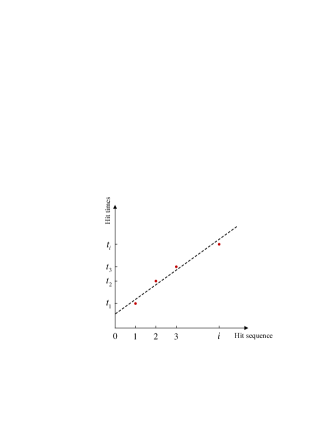
Figure 3: Linear regression model.

$$\left\{\begin{aligned} \hat{\alpha}&=\overline{t}-\hat{\beta}\cdot\overline{i}\\ \hat{\beta}&=\frac{\overline{i\cdot t}-\overline{i}\cdot\overline{t}}{\overline{i^{2}}-(\overline{i})^{2}},\end{aligned}\right.$$ (19)

TABLE II: Comparison of estimator properties ($\hat{\mu}$).

  $\hat{\mu}$ $\mbox{Bias}(\hat{\mu})$ $\mbox{Var}(\hat{\mu})$ $\mbox{MSE}(\hat{\mu})$ $\hat{\mu}_{\mbox{\tiny NE}}=1$ $1-{1\over p}$ $0$ $\frac{(1-p)^{2}}{p^{2}}$ $\hat{\mu}_{\mbox{\tiny MME}}=\hat{\mu}_{\mbox{\tiny MLE}}=\frac{t_{n}-t_{1}}{n-1}$ $0$ $\frac{1-p}{p^{2}(n-1)}$ $\frac{1-p}{p^{2}(n-1)}$ $\hat{\mu}_{\mbox{\tiny LRE}}=\frac{\overline{i\cdot t}-\overline{i}\cdot\overline{t}}{\overline{i^{2}}-(\overline{i})^{2}}$ $0$ $\frac{6(n^{2}+1)(1-p)}{5n(n^{2}-1)p^{2}}$ $\frac{6(n^{2}+1)(1-p)}{5n(n^{2}-1)p^{2}}$  

where the bar symbols denote the average values

$$\left\{\begin{aligned} \overline{i}&=\frac{1}{n}\sum\limits_{i=1}^{n}i,\ \ \ \overline{i^{2}}=\frac{1}{n}\sum\limits_{i=1}^{n}i^{2}\\ \overline{t}&=\frac{1}{n}\sum\limits_{i=1}^{n}t_{i},\ \ \overline{i\cdot t}=\frac{1}{n}\sum\limits_{i=1}^{n}i\cdot t_{i}.\end{aligned}\right.$$ (20)

We then design a linear regression estimator (LRE), i.e.,

$$\hat{\mu}_{\mbox{\tiny LRE}}=\hat{\beta}=\hat{t_{1}}-\hat{t_{0}}.$$ (21)

Thus, the LRE of $t_{0}$ is

$$\hat{t_{0}}_{\mbox{\tiny LRE}}=t_{1}-\hat{\mu}_{\mbox{\tiny LRE}}=t_{1}-\frac{\overline{i\cdot t}-\overline{i}\cdot\overline{t}}{\overline{i^{2}}-(\overline{i})^{2}}.$$ (22)

There is another way to estimate $t_{0}$, which uses the point of interception shown in Fig. 3 as the estimation of $t_{0}$, i.e.,

$$\hat{t_{0}}^{{}^{\prime}}_{\mbox{\tiny LRE}}=\hat{\alpha}=\overline{t}-\hat{\mu}_{\mbox{\tiny LRE}}\cdot\overline{i}.$$ (23)

However, we find that the mean squared error of $\hat{t_{0}}^{{}^{\prime}}_{\mbox{\tiny LRE}}$ increases when $n$ increases. That is, the performance of the estimator worsens with the increasing number of hits, which makes this estimator undesirable.

2.5 Comparison of Estimators

TABLE III: Comparison of estimator properties ($\hat{t_{0}}$).

  $\hat{t_{0}}$ $\mbox{Bias}(\hat{t_{0}})$ $\mbox{Var}(\hat{t_{0}})$ $\mbox{MSE}(\hat{t_{0}})$ $\hat{t_{0}}_{\mbox{\tiny NE}}=t_{1}-\hat{\mu}_{\mbox{\tiny NE}}$ $\frac{1-p}{p}$ $\frac{1-p}{p^{2}}$ $\frac{(1-p)(2-p)}{p^{2}}\ \ \ \ \ \ \ \ \ \ \ \ \ \ \ (\approx\frac{2(1-p)}{p^{2}},\ \mbox{when}\ p\ll 1)$ $\hat{t_{0}}_{\mbox{\tiny MME}}=\hat{t_{0}}_{\mbox{\tiny MLE}}=t_{1}-\hat{\mu}_{\mbox{\tiny MME}}$ $0$ $\frac{1-p}{p^{2}}\cdot\frac{n}{n-1}$ $\frac{1-p}{p^{2}}\cdot\frac{n}{n-1}\ \ \ \ \ \ \ \ \ \ \ \ \ \ \ \ (\approx\frac{1-p}{p^{2}},\ \mbox{when}\ n\gg 1)$ $\hat{t_{0}}_{\mbox{\tiny LRE}}=t_{1}-\hat{\mu}_{\mbox{\tiny LRE}}$ $0$ $\frac{1-p}{p^{2}}\cdot\frac{5n^{3}+6n^{2}-5n+6}{5n(n^{2}-1)}$ $\frac{1-p}{p^{2}}\cdot\frac{5n^{3}+6n^{2}-5n+6}{5n(n^{2}-1)}\ \ (\approx\frac{1-p}{p^{2}},\ \mbox{when}\ n\gg 1)$  

To compare the performance of the naive estimator and our proposed estimators, we compute the bias, the variance, and the mean squared error (MSE). For estimating $\mu$,

$$\left\{\begin{array}[]{l l}\mbox{Bias}(\hat{\mu})\!\!\!\!&=\,\mbox{E}(\hat{\mu})-\mu\\ \mbox{Var}(\hat{\mu})\!\!\!\!&=\,\mbox{E}\,[(\hat{\mu}-\mbox{E}(\hat{\mu}))^{2}]\\ \mbox{MSE}(\hat{\mu})\!\!\!\!&=\,\mbox{E}\,[(\hat{\mu}-\mu)^{2}]=\mbox{Bias}^{2}(\hat{\mu})+\mbox{Var}(\hat{\mu}).\\ \end{array}\right.$$ (24)

Here, the bias denotes the average deviation of the estimator from the true value; the variance indicates the distance between the estimator and its mean; and the MSE characterizes the closeness of the estimated value to the true value. A smaller MSE indicates a better estimator. Table II summarizes the results of NE, MME (or MLE), and LRE for estimating $\mu$. The details of the derivations of Table II are given in Appendix A. It is noted that MME and LRE are unbiased, while NE is biased. Moreover, MME and LRE have a smaller MSE than NE if $n>$ 2 and $p<$ 0.5, a condition that is usually satisfied. Specifically, when $n\rightarrow\infty$, $\mbox{MSE}(\hat{\mu}_{\mbox{\tiny MME}})\rightarrow 0$ and $\mbox{MSE}(\hat{\mu}_{\mbox{\tiny LRE}})\rightarrow 0$, but $\mbox{MSE}(\hat{\mu}_{\mbox{\tiny NE}})\rightarrow(1-p)^{2}/p^{2}$. It is also observed that MME is slightly better than LRE in terms of MSE when $n>$ 2.

Similarly, we compute the bias, the variance, and the MSE of the estimators for estimating $t_{0}$ in Table III. The details of the derivations of Table III are given in Appendix B. We also observe that MME (or MLE) and LRE are unbiased, whereas NE is biased. Moreover, $\mbox{MSE}(\hat{t_{0}}_{\mbox{\tiny MME}})$ and $\mbox{MSE}(\hat{t_{0}}_{\mbox{\tiny LRE}})$ are smaller than $\mbox{MSE}(\hat{t_{0}}_{\mbox{\tiny NE}})$, and $\mbox{MSE}(\hat{t_{0}}_{\mbox{\tiny MME}})$ is the smallest when $n>$ 3 and $p<$ 0.5. Specifically, in practice, Darknet only covers a relatively small portion of the IPv4 address space (i.e., $\omega\ll\Omega$), which leads to $p\ll 1$. Thus, we have the following theorem:

Theorem 1

When the Darknet observes a sufficient number of hits (i.e., $n\gg 1$) and $p\ll 1$,

$$\mbox{MSE}(\hat{t_{0}}_{\mbox{\tiny MME}})\approx\mbox{MSE}(\hat{t_{0}}_{\mbox{\tiny LRE}})\approx\frac{1}{2}\mbox{MSE}(\hat{t_{0}}_{\mbox{\tiny NE}}).$$ (25)

That is, the MSE of our proposed estimators is almost half of that of the naive estimator. That is, our proposed estimators are nearly twice as accurate as the naive estimator in estimating the host infection time.

3 Estimating the Worm Infection Sequence

In this section, we extend our proposed estimators for inferring the worm infection sequence.

3.1 Algorithm

Our algorithm is that we first estimate the infection time of each infected host. Then, we reconstruct the infection sequence based on these infection times. That is, if $\hat{t_{\mbox{\tiny 0}}}_{\mbox{\tiny A}}<\hat{t_{\mbox{\tiny 0}}}_{\mbox{\tiny B}}$, we infer that host A is infected before host B. It is noted that the algorithm used in [25] to infer the worm infection sequence can be regarded as using this approach with the naive estimator.

The naive estimator, however, can potentially fail to infer the worm infection sequence in some cases. Fig. 4 shows an example, where hosts A and B get infected at $t_{\mbox{\tiny 0A}}$ and $t_{\mbox{\tiny 0B}}$, respectively, and $t_{\mbox{\tiny 0A}}<t_{\mbox{\tiny 0B}}$. Moreover, these two infected hosts have scanning rates $s_{\mbox{\tiny A}}<s_{\mbox{\tiny B}}$ such that Darknet observes $t_{\mbox{\tiny 1A}}>t_{\mbox{\tiny 1B}}$. If the naive estimator is used, $\hat{t_{\mbox{\tiny 0}}}_{\mbox{\tiny A}}>\hat{t_{\mbox{\tiny 0}}}_{\mbox{\tiny B}}$, which means that host A is incorrectly inferred to be infected after host B. Intuitively, if our proposed estimators are applied, it is possible to obtain $\hat{t_{\mbox{\tiny 0}}}_{\mbox{\tiny A}}<\hat{t_{\mbox{\tiny 0}}}_{\mbox{\tiny B}}$ and thus recover the real infection sequence.

Figure 4: A scenario of the worm infection sequence.

3.2 Performance Analysis

To analytically show that our estimators are more accurate than the naive estimator in estimating the worm infection sequence, we formulate the problem as a detection problem. Specifically, in Fig. 4, suppose that host B is infected after host A (i.e., $t_{\mbox{\tiny 0A}}<t_{\mbox{\tiny 0B}}$). If $\hat{t_{\mbox{\tiny 0}}}_{\mbox{\tiny A}}<\hat{t_{\mbox{\tiny 0}}}_{\mbox{\tiny B}}$, we call it “success” detection; otherwise, if $\hat{t_{\mbox{\tiny 0}}}_{\mbox{\tiny A}}>\hat{t_{\mbox{\tiny 0}}}_{\mbox{\tiny B}}$, we call it “error” detection. We intend to calculate the probability of error detection for different estimators.

Note that $\delta_{\mbox{\tiny 0A}}=t_{\mbox{\tiny 1A}}-t_{\mbox{\tiny 0A}}$ and $\delta_{\mbox{\tiny 0B}}=t_{\mbox{\tiny 1B}}-t_{\mbox{\tiny 0B}}$ follow the geometric distribution (i.e., Equation (3)) with parameter $p_{\mbox{\tiny A}}$ and $p_{\mbox{\tiny B}}$, respectively. Here, $p_{\mbox{\tiny A}}$ (or $p_{\mbox{\tiny B}}$) is the probability that at least one scan from host A (or B) hits the Darknet in a time unit and follows Equation (1) for random scanning and Equation (2) for localized scanning. Moreover, $p_{\mbox{\tiny A}}$ (or $p_{\mbox{\tiny B}}$) depends on $s_{\mbox{\tiny A}}$ (or $s_{\mbox{\tiny B}}$) so that if $s_{\mbox{\tiny A}}<s_{\mbox{\tiny B}}$, then $p_{\mbox{\tiny A}}<p_{\mbox{\tiny B}}$. Since $\omega\ll\Omega$, we have $p_{\mbox{\tiny A}}\ll 1$ and $p_{\mbox{\tiny B}}\ll 1$. Hence, for simplicity we use the continuous-time analysis and apply the exponential distribution to approximate the geometric distribution for $\delta_{\mbox{\tiny 0A}}$ and $\delta_{\mbox{\tiny 0B}}$ [31], i.e.,

$$f(x;\lambda)=\left\{\begin{array}[]{l l}\lambda e^{-\lambda x},&\quad x\geq 0\\ 0,&\quad x<0,\\ \end{array}\right.$$ (26)

where $\lambda=p_{\mbox{\tiny A}}$ or $p_{\mbox{\tiny B}}$.

                 

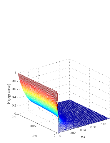
(a) $\mbox{Pr}_{\mbox{\tiny NE}}(\mbox{error})$.

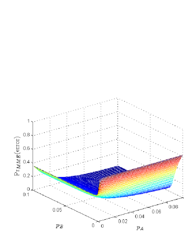
(b) $\mbox{Pr}_{\mbox{\tiny MME}}(\mbox{error})$.

Figure 5: Analytical results of $\mbox{Pr}(\mbox{error})$ when changing $p_{\mbox{\tiny A}}$ and $p_{\mbox{\tiny B}}$ ($\tau$ = 50 time units).

To calculate the probability of error detection for different estimators, we first define a new random variable

$$Z=\delta_{\mbox{\tiny 0A}}-\delta_{\mbox{\tiny 0B}},$$ (27)

and calculate its probability density function (pdf) $f_{\mbox{\tiny Z}}(z)$. From Equation (26), we can obtain the pdf of $\delta_{\mbox{\tiny 0B}}^{\prime}=-\delta_{\mbox{\tiny 0B}}$, which is

$$f_{\delta_{\mbox{\tiny 0B}}^{\prime}}(x)=\left\{\begin{array}[]{l l}p_{\mbox{\tiny B}}\,e^{p_{\mbox{\tiny B}}x},&\quad x\leq 0\\ 0,&\quad x>0.\\ \end{array}\right.$$ (28)

Since $\delta_{\mbox{\tiny 0A}}$ and $\delta_{\mbox{\tiny 0B}}^{\prime}$ are independent, the pdf of $Z=\delta_{\mbox{\tiny 0A}}+\delta_{\mbox{\tiny 0B}}^{\prime}$ is given by the convolution of $f_{\delta_{\mbox{\tiny 0A}}}(x)$ and $f_{\delta_{\mbox{\tiny 0B}}^{\prime}}(x)$, i.e.,

$$f_{\mbox{\tiny Z}}(z)=\int_{-\infty}^{+\infty}f_{\delta_{\mbox{\tiny 0A}}}(x)f_{\delta_{\mbox{\tiny 0B}}^{\prime}}(z-x)\,dx.$$ (29)

For $z\geq 0$, this yields

$$f_{\mbox{\tiny Z}}(z) = \int_{z}^{+\infty}p_{\mbox{\tiny A}}\,e^{-p_{\mbox{\tiny A}}x}\cdot p_{\mbox{\tiny B}}\,e^{p_{\mbox{\tiny B}}(z-x)}\,dx$$ (30)

$$= \textstyle\frac{p_{\mbox{\tiny A}}p_{\mbox{\tiny B}}}{p_{\mbox{\tiny A}}+p_{\mbox{\tiny B}}}\,e^{-p_{\mbox{\tiny A}}z}.$$

For $z<0$, we obtain

$$f_{\mbox{\tiny Z}}(z) = \int_{0}^{+\infty}p_{\mbox{\tiny A}}\,e^{-p_{\mbox{\tiny A}}x}\cdot p_{\mbox{\tiny B}}\,e^{p_{\mbox{\tiny B}}(z-x)}\,dx$$ (31)

$$= \textstyle\frac{p_{\mbox{\tiny A}}p_{\mbox{\tiny B}}}{p_{\mbox{\tiny A}}+p_{\mbox{\tiny B}}}\,e^{p_{\mbox{\tiny B}}z}.$$

Hence,

$$f_{\mbox{\tiny Z}}(z)=\left\{\begin{array}[]{l l}\frac{p_{\mbox{\tiny A}}p_{\mbox{\tiny B}}}{p_{\mbox{\tiny A}}+p_{\mbox{\tiny B}}}\,e^{-p_{\mbox{\tiny A}}z},&z\geq 0\\ \frac{p_{\mbox{\tiny A}}p_{\mbox{\tiny B}}}{p_{\mbox{\tiny A}}+p_{\mbox{\tiny B}}}\,e^{p_{\mbox{\tiny B}}z},&z<0.\\ \end{array}\right.$$ (32)

                          

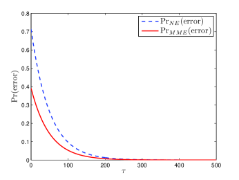
(a) $\mbox{Pr}(\mbox{error})$ ($p_{\mbox{\tiny A}}=0.02$ and $p_{\mbox{\tiny B}}=0.05$).

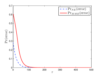
(b) $\mbox{Pr}(\mbox{error})$ ($p_{\mbox{\tiny A}}=0.05$ and $p_{\mbox{\tiny B}}=0.02$).

Figure 6: Analytical results of $\mbox{Pr}(\mbox{error})$ when changing $\tau$.

3.2.1 Naive Estimator

The naive estimator uses $\hat{t_{\mbox{\tiny 0}}}=t_{\mbox{\tiny 1}}-1$ to estimate $t_{\mbox{\tiny 0}}$. Thus, the probability of error detection is

$$\mbox{Pr}_{\mbox{\tiny NE}}(\mbox{error})=\mbox{Pr}(t_{\mbox{\tiny 1A}}-1>t_{\mbox{\tiny 1B}}-1)=\mbox{Pr}(\delta_{\mbox{\tiny 0A}}>\tau+\delta_{\mbox{\tiny 0B}}),$$ (33)

where $\tau=t_{\mbox{\tiny 0B}}-t_{\mbox{\tiny 0A}}$, the time interval between the infection of host A and host B; and $\tau>0$. We then have

$$\mbox{Pr}_{\mbox{\tiny NE}}(\mbox{error}) = \mbox{Pr}(\delta_{\mbox{\tiny 0A}}-\delta_{\mbox{\tiny 0B}}>\tau)$$ (34)

$$= \mbox{Pr}(Z>\tau)$$

$$= \int_{\tau}^{+\infty}\textstyle\frac{p_{\mbox{\tiny A}}p_{\mbox{\tiny B}}}{p_{\mbox{\tiny A}}+p_{\mbox{\tiny B}}}\,e^{-p_{\mbox{\tiny A}}z}\,dz$$

$$= \textstyle\frac{p_{\mbox{\tiny B}}}{p_{\mbox{\tiny A}}+p_{\mbox{\tiny B}}}\,e^{-p_{\mbox{\tiny A}}\tau}.$$

Note that another way to derive $\mbox{Pr}_{\mbox{\tiny NE}}(\mbox{error})$ is based on the memoryless property of the exponential distribution and $\mbox{Pr}(\delta_{\mbox{\tiny 0A}}>\delta_{\mbox{\tiny 0B}})=p_{\mbox{\tiny B}}/(p_{\mbox{\tiny A}}+p_{\mbox{\tiny B}})$, i.e.,

$$\mbox{Pr}_{\mbox{\tiny NE}}(\mbox{error})=\mbox{Pr}(\delta_{\mbox{\tiny 0A}}>\tau+\delta_{\mbox{\tiny 0B}})=\mbox{Pr}(\delta_{\mbox{\tiny 0A}}>\tau)\mbox{Pr}(\delta_{\mbox{\tiny 0A}}>\delta_{\mbox{\tiny 0B}}),$$ (35)

which leads to the same result.

3.2.2 Proposed Estimators

We assume that Darknet observes a sufficient number of scans from hosts A and B so that our proposed estimators can estimate $\mu_{\mbox{\tiny A}}$ (i.e., $\frac{1}{p_{\mbox{\tiny A}}}$) and $\mu_{\mbox{\tiny B}}$ (i.e., $\frac{1}{p_{\mbox{\tiny B}}}$) accurately. Then, the probability of error detection of our proposed estimators is

$$\mbox{Pr}_{\mbox{\tiny MME}}(\mbox{error}) = \mbox{Pr}_{\mbox{\tiny MLE}}(\mbox{error})=\mbox{Pr}_{\mbox{\tiny LRE}}(\mbox{error})$$ (36)

$$= \mbox{Pr}(t_{\mbox{\tiny 1A}}-\textstyle{1\over p_{\mbox{\tiny A}}}>t_{\mbox{\tiny 1B}}-{1\over p_{\mbox{\tiny B}}})$$

$$= \mbox{Pr}(\delta_{\mbox{\tiny 0A}}-\delta_{\mbox{\tiny 0B}}>\tau+\textstyle{1\over p_{\mbox{\tiny A}}}-\textstyle{1\over p_{\mbox{\tiny B}}})$$

$$= \textstyle\mbox{Pr}(Z>\tau+\frac{p_{\mbox{\tiny B}}-p_{\mbox{\tiny A}}}{p_{\mbox{\tiny A}}p_{\mbox{\tiny B}}})$$

$$= \int_{\tau+\frac{p_{\mbox{\tiny B}}-p_{\mbox{\tiny A}}}{p_{\mbox{\tiny A}}p_{\mbox{\tiny B}}}}^{+\infty}f_{\mbox{\tiny Z}}(z)\,dz.$$

When $\tau+\frac{p_{\mbox{\tiny B}}-p_{\mbox{\tiny A}}}{p_{\mbox{\tiny A}}p_{\mbox{\tiny B}}}\geq 0$,

$$\mbox{Pr}_{\mbox{\tiny MME}}(\mbox{error}) = \int_{\tau+\frac{p_{\mbox{\tiny B}}-p_{\mbox{\tiny A}}}{p_{\mbox{\tiny A}}p_{\mbox{\tiny B}}}}^{+\infty}\textstyle\frac{p_{\mbox{\tiny A}}p_{\mbox{\tiny B}}}{p_{\mbox{\tiny A}}+p_{\mbox{\tiny B}}}\,e^{-p_{\mbox{\tiny A}}z}\,dz$$ (37)

$$= \textstyle\frac{p_{\mbox{\tiny B}}}{p_{\mbox{\tiny A}}+p_{\mbox{\tiny B}}}\,e^{-p_{\mbox{\tiny A}}\big{(}\tau+\frac{p_{\mbox{\tiny B}}-p_{\mbox{\tiny A}}}{p_{\mbox{\tiny A}}p_{\mbox{\tiny B}}}\big{)}}.$$

When $\tau+\frac{p_{\mbox{\tiny B}}-p_{\mbox{\tiny A}}}{p_{\mbox{\tiny A}}p_{\mbox{\tiny B}}}<0$,

$$\mbox{Pr}_{\mbox{\tiny MME}}(\mbox{error}) = \int_{\tau+\frac{p_{\mbox{\tiny B}}-p_{\mbox{\tiny A}}}{p_{\mbox{\tiny A}}p_{\mbox{\tiny B}}}}^{0}\textstyle\frac{p_{\mbox{\tiny A}}p_{\mbox{\tiny B}}}{p_{\mbox{\tiny A}}+p_{\mbox{\tiny B}}}\,e^{p_{\mbox{\tiny B}}z}\,dz+$$ (38)

$$\int_{0}^{+\infty}\textstyle\frac{p_{\mbox{\tiny A}}p_{\mbox{\tiny B}}}{p_{\mbox{\tiny A}}+p_{\mbox{\tiny B}}}\,e^{-p_{\mbox{\tiny A}}z}\,dz$$

$$= \!\!\!\!\textstyle\frac{1}{p_{\mbox{\tiny A}}+p_{\mbox{\tiny B}}}\Big{(}p_{\mbox{\tiny A}}+p_{\mbox{\tiny B}}-p_{\mbox{\tiny A}}\,e^{p_{\mbox{\tiny B}}\big{(}\tau+\frac{p_{\mbox{\tiny B}}-p_{\mbox{\tiny A}}}{p_{\mbox{\tiny A}}p_{\mbox{\tiny B}}}\big{)}}\Big{)}.$$

3.2.3 Performance Comparison

Since $\mbox{Pr}_{\mbox{\tiny NE}}(\mbox{error})=\mbox{Pr}(Z>\tau)$ and $\mbox{Pr}_{\mbox{\tiny MME}}(\mbox{error})=\textstyle\mbox{Pr}\big{(}Z>\tau+\frac{p_{\mbox{\tiny B}}-p_{\mbox{\tiny A}}}{p_{\mbox{\tiny A}}p_{\mbox{\tiny B}}}\big{)}$, for a given $\tau$ ($\tau>0$), comparing Equation (34) with Equations (37) and (38),

$$\left\{\begin{array}[]{l l}\mbox{Pr}_{\mbox{\tiny NE}}(\mbox{error})>\mbox{Pr}_{\mbox{\tiny MME}}(\mbox{error}),&p_{\mbox{\tiny A}}<p_{\mbox{\tiny B}}\\ \mbox{Pr}_{\mbox{\tiny NE}}(\mbox{error})<\mbox{Pr}_{\mbox{\tiny MME}}(\mbox{error}),&p_{\mbox{\tiny A}}>p_{\mbox{\tiny B}}.\\ \end{array}\right.$$ (39)

Hence, it is unclear which estimator is better based on the expressions of $\mbox{Pr}_{\mbox{\tiny NE}}(\mbox{error})$ and $\mbox{Pr}_{\mbox{\tiny MME}}(\mbox{error})$. However, we can compare the performance of our estimators with the naive estimator through numerical analysis. We first demonstrate the probabilities of error detection (i.e., $\mbox{Pr}_{\mbox{\tiny NE}}(\mbox{error})$ and $\mbox{Pr}_{\mbox{\tiny MME}}(\mbox{error})$) as the functions of $p_{\mbox{\tiny A}}$ and $p_{\mbox{\tiny B}}$ in Fig. 5, where $\tau$ = 50 time units. It can be seen that for the naive estimator, when host A hits the Darknet with a very low probability, $\mbox{Pr}_{\mbox{\tiny NE}}(\mbox{error})$ is almost 1 regardless of $p_{\mbox{\tiny B}}$. However, the worst case of $\mbox{Pr}_{\mbox{\tiny MME}}(\mbox{error})$ is slightly above 0.6 when $p_{\mbox{\tiny B}}$ is small. Moreover, we show the probabilities of error detection as a function of $\tau$ with a given pair of $p_{\mbox{\tiny A}}$ and $p_{\mbox{\tiny B}}$ in Fig. 6. The performance of two estimators improves as $\tau$ increases. Furthermore, the sum of the integral $\int_{0}^{500}\mbox{Pr}_{\mbox{\tiny NE}}(\mbox{error})\,d\tau$ of the two figures is 41.43, while the sum of the integral $\int_{0}^{500}\mbox{Pr}_{\mbox{\tiny MME}}(\mbox{error})\,d\tau$ in these two cases is only 34.76. This shows that the improvement gain of our estimators over the naive estimator when $p_{\mbox{\tiny A}}<p_{\mbox{\tiny B}}$ outweighs the degradation suffered when $p_{\mbox{\tiny A}}>p_{\mbox{\tiny B}}$, indicating the benefits of applying our estimators.

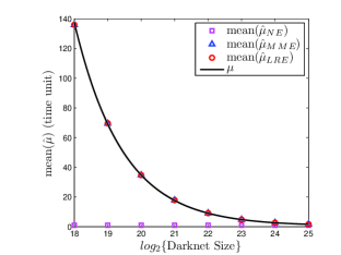
(a) Comparison of $\hat{\mu}$.

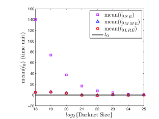
(b) Comparison of $\hat{t_{0}}$.

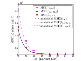
(c) Comparison of $\mbox{MSE}(\hat{t_{0}})$.

Figure 7: Simulation results of changing the Darknet size for random scanning (all cases are for scanning rate: 358 scans/min, observation window size: 800 mins).

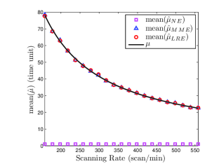
(a) Comparison of $\hat{\mu}$.

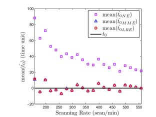
(b) Comparison of $\hat{t_{0}}$.

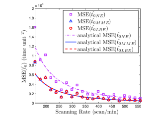
(c) Comparison of $\mbox{MSE}(\hat{t_{0}})$.

Figure 8: Simulation results of changing the scanning rate for random scanning (all cases are for Darknet size: $2^{20}$ IP addresses, observation window size: 800 mins).

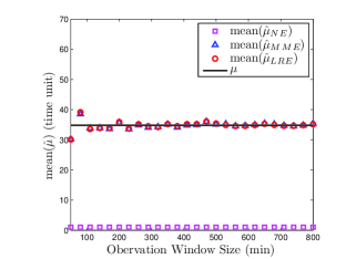
(a) Comparison of $\hat{\mu}$.

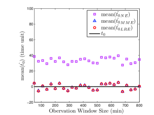
(b) Comparison of $\hat{t_{0}}$.

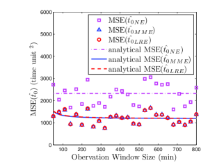
(c) Comparison of $\mbox{MSE}(\hat{t_{0}})$.

Figure 9: Simulation results of changing the observation window size for random scanning (all cases are for scanning rate: 358 scans/min, Darknet size: $2^{20}$ IP addresses).

(a) Comparison of $\mbox{MSE}(\hat{t_{0}})$.

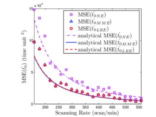
(b) Comparison of $\mbox{MSE}(\hat{t_{0}})$.

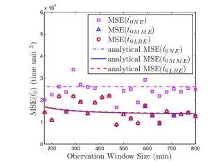
(c) Comparison of $\mbox{MSE}(\hat{t_{0}})$.

Figure 10: (a) Simulation results of changing the Darknet size for localized scanning ($p_{a}$ = 0.7, scanning rate: 358 scans/min, observation window size: 800 mins). (b) Simulation results of changing the scanning rate for localized scanning ($p_{a}$ = 0.7, Darknet size: $2^{20}$ IP addresses, observation window size: 800 mins). (c) Simulation results of changing the observation window size for localized scanning ($p_{a}$ = 0.7, scanning rate: 358 scans/min, Darknet size: $2^{20}$ IP addresses).

Note that $p_{\mbox{\tiny A}}$, $p_{\mbox{\tiny B}}$, and $\tau$ can be random variables. To evaluate the overall performance of each estimator, we consider the average probability of error detection over $p_{\mbox{\tiny A}}$, $p_{\mbox{\tiny B}}$, and $\tau$, i.e.,

$$\mbox{E}\,[\mbox{Pr}(\mbox{error})]=\int_{\tau}\int_{p_{\mbox{\tiny A}}}\int_{p_{\mbox{\tiny B}}}\mbox{Pr}(\mbox{error})\cdot f(p_{\mbox{\tiny A}},p_{\mbox{\tiny B}},\tau)\,\,d\,p_{\mbox{\tiny B}}\,d\,p_{\mbox{\tiny A}}\,d\tau.$$ (40)

Since $p_{\mbox{\tiny A}}$, $p_{\mbox{\tiny B}}$, and $\tau$ are independent,

$$f(p_{\mbox{\tiny A}},p_{\mbox{\tiny B}},\tau)=f(p_{\mbox{\tiny A}})\cdot f(p_{\mbox{\tiny B}})\cdot f(\tau).$$ (41)

We then consider some cases in which we are interested and apply the numerical integration toolbox in Matlab [32] to calculate the triple integration. For example, we assume that $s_{\mbox{\tiny A}}$ and $s_{\mbox{\tiny B}}$ follow a normal distribution $N(u,\sigma^{2})$ and $\tau$ is uniform over $(0,\tau_{1}]$. We find that when $u$, $\sigma^{2}$, and $\tau_{1}$ are set to realistic values, we always have

$$\mbox{E}\,[\mbox{Pr}_{\mbox{\tiny NE}}(\mbox{error})]>\mbox{E}\,[\mbox{Pr}_{\mbox{\tiny MME}}(\mbox{error})].$$ (42)

That is, our proposed estimators perform better than NE on average, which will further be verified in Section 4 through simulations.

Moreover, in Fig. 5(a), it can be seen that the majority of detection error for the naive estimator comes from the case that $p_{\mbox{\tiny A}}<p_{\mbox{\tiny B}}$. Specifically, it is obvious to derive the following theorem from Equations (34) and (37).

Theorem 2

When $p_{\mbox{\tiny A}}<p_{\mbox{\tiny B}}$,

$$\mbox{Pr}_{\mbox{\tiny MME}}(\mbox{error}) = \mbox{Pr}_{\mbox{\tiny MLE}}(\mbox{error})=\mbox{Pr}_{\mbox{\tiny LRE}}(\mbox{error})$$ (43)

$$= \mbox{Pr}_{\mbox{\tiny NE}}(\mbox{error})\cdot e^{-\big{(}1-\frac{p_{\mbox{\tiny A}}}{p_{\mbox{\tiny B}}}\big{)}}.$$

That is, the error probability is decreased by a factor of $e^{-\big{(}1-\frac{p_{\mbox{\tiny A}}}{p_{\mbox{\tiny B}}}\big{)}}$ by applying our estimators as compared with the naive estimator.

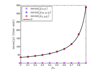
(a) Comparison of $\hat{\mu}$.

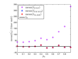
(b) Comparison of $\hat{t_{0}}$.

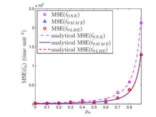
(c) Comparison of $\mbox{MSE}(\hat{t_{0}})$.

Figure 11: Simulation results of changing $p_{a}$ for localized scanning (all cases are for scanning rate: 358 scans/min, Darknet size: $2^{20}$ IP addresses, observation window size: 800 mins).

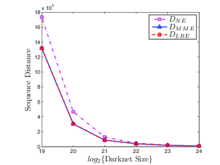
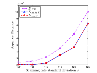
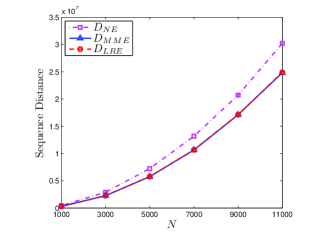
Figure 12: Simulation results of the sequence distance for random scanning. (a) Changing the Darknet size ($N$ = 1,000, observation window size: 1,600 mins, scanning rate: $N(358,115^{2})$). (b) Changing the scanning rate standard deviation ($N$ = 1,000, observation window size: 1,600 mins, Darknet size: $2^{20}$ IP addresses). (c) Changing the length of the infection sequence considered (observation window size: 1,600 mins, Darknet size: $2^{20}$ IP addresses, scanning rate: $N(358,115^{2})$).

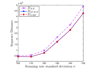
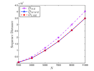
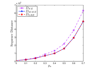
Figure 13: Simulation results of the sequence distance for localized scanning. (a) Changing the scanning rate standard deviation ($p_{a}$ = 0.7, $N$ = 1,000, observation window size: 1,000 mins, Darknet size: $2^{24}$ IP addresses). (b) Changing the length of the infection sequence considered ($p_{a}$ = 0.7, observation window size: 1,000 mins, Darknet size: $2^{24}$ IP addresses, scanning rate: $N(358,115^{2})$). (c) Changing the $p_{a}$ ($N$ = 1,000, observation window size: 1,000 mins, Darknet size: $2^{24}$ IP addresses, scanning rate: $N(358,115^{2})$).

4 Simulation Results

In this section, we use simulations to verify our analytical results and then apply estimators to identify the patient zero or the hitlist. As far as we know, there is no publicly available data to show the real worm infection sequence. That is, there is no dataset available with the real infection sequence to serve as the ground truth and a comparison basis for performance evaluation. Therefore, we apply empirical simulations to provide the simulated worm infection time and infection sequence.

4.1 Estimating the Host Infection Time

We evaluate the performance of estimators in estimating the host infection time. For the case of random-scanning worms, we simulate the behavior of a host infected by the Code Red v2 worm. The host is infected at time tick 0 and uses a constant scanning rate. The time unit is set to 20 seconds. The Darknet records hit times during an observation window. We consider the effects of the Darknet size, the scanning rate, and the observation window size on the performance of the estimators. The results are averaged over 100 independent runs. Fig. 7 compares the performance of NE, MME, and LRE with different Darknet sizes from $2^{18}$ to $2^{25}$, a scanning rate of 358 scans/min, and an observation window size of 800 mins. The three sub-figures show the mean of estimators for $\mu$, the mean of estimators for $t_{0}$, and the MSE of estimators for $t_{0}$. Fig. 8 compares the three estimators with different scanning rates from 158 scans/min to 558 scans/min, a Darknet size of $2^{20}$, and an observation window size of 800 mins. Similarly, Fig. 9 is with different observation window sizes from 50 mins to 800 mins, a scanning rate of 358 scans/min, and a Darknet size of $2^{20}$. It is observed that for all cases, our proposed estimators have a better performance (i.e., unbiasedness and smaller MSE) than the naive estimator in estimating the host infection time. Specifically, the simulation results verify Theorem 1, i.e., that the MSE of our estimators is almost half of that of the naive estimator, when the observation window size is sufficiently large (e.g., $>$ 200 mins).

Next, we study a host infected by localized-scanning worms and adopt the same simulation parameters and settings as the above. The main difference is that here the host preferentially searches for vulnerable hosts in the “local” address space with a probability $p_{a}$. In Fig. 10, $p_{a}$ is set to 0.7, and we compare MSE($\hat{t_{0}}$) for different estimators. We find that the results are similar to those for the random-scanning case shown in Fig.s 7-9. The MSE($\hat{t_{0}}$) in Fig. 10, however, is larger for all cases since the localized-scanning worm hits the Darknet less frequently than the random-scanning worm. In Fig. 11, we compare the performance of NE, MME, and LRE with different $p_{a}$ from 0 to 0.9, a scanning rate of 358 scans/min, a Darknet size of $2^{20}$, and an observation window size of 800 mins. Similarly, the results show that our estimators are unbiased and the MSE of our estimators is almost half of that of the naive estimator.

                 

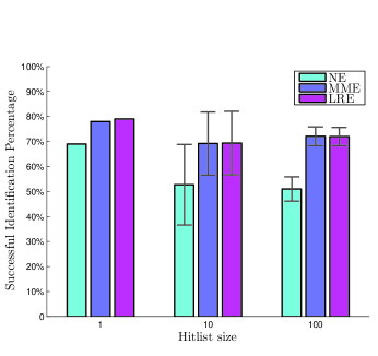
(a) Random scanning.

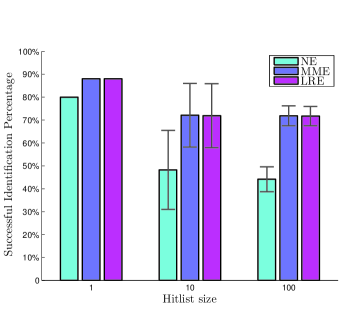
(b) Localized scanning.

Figure 14: Comparison of estimators when changing the hitlist size. (a) Random scanning (all cases are for Darknet size: $2^{20}$ IP addresses, observation window size: 1000 mins, hitlist hosts scanning rate: $N(50,20^{2})$, other hosts scanning rate: $N(358,110^{2})$). (b) Localized scanning (all cases are for $p_{a}$ = 0.7, Darknet size: $2^{24}$ IP addresses, observation window size: 1000 mins, hitlist hosts scanning rate: $N(50,20^{2})$, other hosts scanning rate: $N(358,110^{2})$).

4.2 Estimating the Worm Infection Sequence

We evaluate the performance of our algorithms in estimating the worm infection sequence and simulate the propagation of the Code Red v2 worm. The simulator is extended from the code provided by [33], where the parameter setting is based on the worm characteristics. The Code Red worm has a vulnerable population of 360,000. Different infected hosts may have different scanning rates. Thus, we assign a scanning rate (scans/min) from a normal distribution $N(358,\sigma^{2})$ to a newly infected host. Moreover, we start our simulation at time tick 0 from one infected host. The time unit is set to 20 seconds. Detailed information about how the parameters are chosen can be found in Section VII of [22]. Each point in Fig. 12 is averaged over 20 independent runs. Table IV gives the results of a sample run with a Darknet size of $2^{20}$, an observation window size of 1,600 mins, and $\sigma$ = 110. In the table, $S_{i}$ is the actual infection sequence (i.e., $S_{i}=i$), whereas $\hat{S_{i}}$ is the estimated sequence. In this example, we find that MME and LRE can pinpoint the patient zero successfully, while NE fails.

TABLE IV: A sample run of simulations for random scanning.

  $S_{i}$ $\hat{S_{i}}_{\mbox{\tiny NE}}$ $\hat{S_{i}}_{\mbox{\tiny MME}}$ $\hat{S_{i}}_{\mbox{\tiny LRE}}$ $t_{0}$ $\hat{t_{0}}_{\mbox{\tiny NE}}$ $\hat{t_{0}}_{\mbox{\tiny MME}}$ $\hat{t_{0}}_{\mbox{\tiny LRE}}$ 1 2 1 1 0 114 20 20 2 1 2 2 85 98 74 73 3 3 3 3 105 165 116 116 : : : : : : : : 520 498 533 534 593 622 589 589 521 433 488 477 594 611 581 580 : : : : : : : :  

To compare the performance of estimators quantitatively, we consider a simple $l_{1}$ sequence distance, i.e.,

$$D=\sum\limits_{i=1}^{N}{\Big{|}{S_{i}-\hat{S_{i}}}\Big{|}},$$ (44)

where $N$ is the length of the infection sequence considered. Note that the smaller the sequence distance is, the better the estimator performance will be. Fig. 12(a) shows the sequence distances of NE, MME, and LRE with varying Darknet sizes from $2^{19}$ to $2^{24}$, an observation window size of 1,600 mins, $N$ = 1,000, and $\sigma$ = 115. It is observed that when the Darknet size increases, the performance of all estimators improves dramatically. Moreover, the performance of MME and LRE is always better than that of NE. For example, when the Darknet size equals $2^{19}$, MME and LRE improve the inference accuracy by 24%, compared with NE. Fig. 12(b) demonstrates the sequence distances of these three estimators by changing the standard deviation of the scanning rate (i.e., $\sigma$) from 100 to 125. In the figure, the Darknet size is $2^{20}$, the observation window size is 1,600 mins, and $N$ = 1,000. It is noted that when $\sigma$ increases, the performance of all estimators deteriorates. The performance of MME and LRE, however, is always better than that of NE. For example, when $\sigma$ = 120, MME and LRE reduce the sequence distance by 30%, compared with NE. In Fig. 12(c), we increase the length of the infection sequence considered, $N$, from 1,000 to 11,000. Here the Darknet size is $2^{20}$, the observation window size is 1,600 mins, and $\sigma$ = 115. It is intuitive that the sequence distances of all estimators become larger as $N$ increases. However, MME and LRE are always better than NE.

Next, we extend our simulator to imitate the spread of localized-scanning worms. Specifically, we consider /8 localized-scanning worms and a centralized /8 Darknet with $2^{24}$ IP addresses. We still use the Code Red v2 worm parameters and the same setting as random scanning, except that the observation window size is 1,000 mins (this is because localized-scanning worms spread faster). The distribution of vulnerable hosts is extracted from the dataset provided by DShield [34]. DShield obtains the information of vulnerable hosts by aggregating logs from more than 1,600 intrusion detection systems distributed throughout the Internet. Specifically, we use the dataset with port 80 (HTTP) that is exploited by the Code Red v2 worm to generate the vulnerable-hosts distribution. Each point in Fig. 13 is averaged over 20 independent runs. Fig. 13 compares the sequence distances of different estimators for localized scanning. Specifically, the results in Fig. 13(a) and (b) are similar to those in Fig. 12(b) and (c). In Fig. 13(c), we compare the performance of the estimators by increasing $p_{a}$ from 0 to 0.7. Here, $N$ = 1,000, and $\sigma$ = 115. It is observed that the sequence distances of all estimators increase as $p_{a}$ becomes larger. However, our estimators are always better than NE. For example, when $p_{a}$ = 0.5, MME and LRE increase the inference accuracy by 27%, compared with NE.

Therefore, our proposed estimators perform much better than the naive estimator for both random-scanning and localized-scanning worms in estimating the worm infection sequence.

4.3 Identifying the Patient Zero or the Hitlist

As discussed in Section 1, a smart worm can assign lower scanning rates to the initially infected host(s) and higher scanning rates to other infected hosts. In this way, the Darknet might observe later infected hosts first, and therefore the smart worm would weaken the performance of the naive estimator. In Fig. 14, we compare the performance of estimators in identifying the hitlist of such a smart worm. Specifically, the worm assigns scanning rates from $N(50,20^{2})$ to the host(s) on the hitlist and scanning rates from $N(358,110^{2})$ to other infected hosts. Then, we calculate the percentage of the host(s) on the hitlist that are successfully identified by an estimator. For example, if the size of the hitlist is 100 and 50 hosts that belong to the hitlist are identified among the first 100 hosts of the estimated infection sequence, the successful identification percentage of the estimator is 50%. The results are averaged over 100 independent runs. Fig. 14(a) shows the case of random scanning, where the Darkent size is $2^{20}$ and the observation window size is 1,000 mins. It is seen that our estimators have a higher successful identification percentage and a smaller variance than the naive estimator. For instance, when the size of the hitlist is 1 (i.e., the worm starts from the patient zero), MME and LRE can pinpoint the patient zero around 80% of the time, while NE can detect it only 70% of the time. When the size of the hitlist is 10 or 100, compared with NE, our proposed estimators increase the number of successfully identified hosts from 5 to 7 or 51 to 72, and reduce the variance from 2.6 to 1.6 or 23 to 13, respectively. Fig. 14(b) shows the results of localized scanning, where the Darkent size is $2^{24}$ and $p_{a}$ = 0.7, and all other parameters are the same as the case of random scanning. The results are similar to those in Fig. 14(a). Therefore, the simulation results demonstrate that our proposed estimators are much more effective in identifying the histlist of the smart worm than the naive estimator.

5 Discussions

In this section, we first analyze the chance that Darknet misses an infected host and then discuss the limitations and the extensions of our proposed estimators.

5.1 Host Missing Probability

By applying Darknet observations, we have made an assumption: The infected host will hit the Darknet. Then, an intuitive question would be: What is the probability that the Darknet misses an infected host within a given observation window?

We consider the case of localized scanning and regard random scanning as a special case of localized scanning when $p_{a}$ = 0. The probability for a scan from an infected host to hit the Darknet is $(1-p_{a})\cdot\omega/\Omega$; and then the probability that the Darknet misses observing the host in a time unit is $(1-(1-p_{a})\cdot{\omega}/{\Omega})^{s}$. Thus, the host missing probability (i.e., the probability that the Darknet misses the infected host in a $k$ time units observation window) is

$$\mbox{Pr}_{\mbox{\tiny LS}}(\mbox{missing})=\Big{(}1-(1-p_{a})\cdot\frac{\omega}{\Omega}\Big{)}^{s\cdot k}.$$ (45)

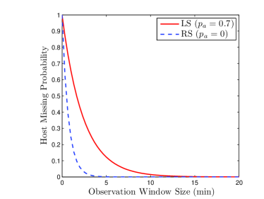
Figure 15: Host missing probability ($p_{a}$ = 0.7, Darknet size: $2^{24}$ IP addresses, scanning rate: 358 scans/min).

In Fig. 15, we show the host missing probability as the observation window size changes. In this example, we set $\omega$ = $2^{24}$, time unit = 20 seconds, and $s$ = 358 scans/min. We find that if $p_{a}$ = 0.7, the infected host will almost hit the Darknet for sure when the observation window size is larger than 20 mins. If $p_{a}$ = 0, which is the case of random scanning, a 5-min observation window is sufficient to guarantee the capture of the infected host. Therefore, in our previous analysis and simulation, the assumption that the Darknet can observe scans from the infected host, especially at the early stage, is reasonable. Moreover, our estimator can still work even for self-stopping worms [35].

5.2 Estimator Limitations and Extensions

Our proposed estimators are built based on some assumptions listed in Section 2. Attackers that design future worms may exploit these assumptions to weaken the accuracy of our estimators. In the following, we discuss some limitations of our estimators and the potential extensions.

5.2.1 Darknet Avoidance

The majority of active worms up to date do not attempt to avoid the detection of Darknet. As a result, CAIDA’s network telescopes have been observing many active Internet worms such as Code Red, Slammer, Witty, and even recently the Conficker worm (also known as the April Fool’s worm). Most worms apply random scanning and localized scanning, and Darknet can observe the traffic from such worms.

Recent work, however, has shown that attackers can potentially detect the locations of Darknet or network sensors [36]. Thus, a future worm can be specially designed to avoid scanning the address space of the Darknet. The countermeasure against such an intelligent worm is to apply the distributed Darknet instead of the centralized Darknet [23]. That is, unused IP addresses in many subnets are used to observe worm traffic, which is then reported to a collection center for further processing. A prototype of distributed Darknet has been designed and evaluated in [37].

5.2.2 Scanning Rate Variation

Although there have been no observations of worms that use scanning rate variation mechanisms (i.e., the scanning rate of an individual infected host is time-variant) [29], future worms may employ such schemes to invalidate our basic assumption and thus weaken the performance of our estimators. Changing the scanning rate, however, introduces additional complexity to worm design and can slow down worm spreading. Moreover, if the change of scanning rates is relatively slow, our estimators can be enhanced with the change-point detection [38] to detect and track when the scanning rate has a significant change and then apply the early observations to derive the infection time of an infected host.

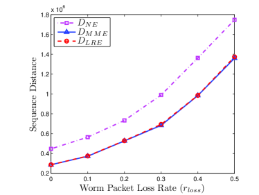
Figure 16: Simulation results of the sequence distances of different estimators varying with the worm packet loss rate. ($N$ = 1,000, observation window size: 1,600 mins, scanning rate: $N(358,115^{2})$, Darknet size: $2^{20}$ IP addresses).

5.2.3 Measurement Errors

The measurement errors can affect the performance of estimators. There are two types of measurement errors. The false positive denotes that Darknet incorrectly classifies the traffic from a benign host as worm traffic, whereas the false negative is that Darknet incorrectly classifies worm traffic as benign traffic or misses worm traffic due to congestion or device malfunction.

For the false positives, most of time we can distinguish worm traffic from other traffic. First, our estimation techniques are used as a form of post-mortem analysis on worm records logged by Darknet. As a result, we can limit our analysis to the records logged during the outbreak of the worm when it is most rampant. More importantly, worm packages always contain information about infection vectors that distinguish worm traffic from other traffic. For example, the Witty worm uses a source port of 4,000 to attack Internet Security Systems firewall products [16]. It is very unlikely that a benign host uses a source port of 4,000. By filtering the records based on infection vectors specific to the worm under investigation, we can eliminate most of the effects of false positives on Darknet observations.

False negatives are much harder to eliminate. A packet towards Darknet may be lost due to congestion caused by the worm (such as the Slammer worm [1]) or the malfunction of Darknet monitoring devices. To study the effects of false negatives, we modify our simulator to mimic the packet loss and evaluate the performance of our estimators under false negatives. Here we assume that the loss rate of the worm packets towards Darknet (denoted as $r_{\mbox{\scriptsize loss}}$) is the same for each infected host. Fig. 16 shows how the sequence distances of different estimators vary with the worm packet loss rate. The results are averaged over 20 independent runs. It is intuitive that when the packet loss rate becomes larger, the performance of all estimators worsens. Our proposed estimators, however, always perform much better than NE. For example, compared with NE, our estimators (i.e., MME and LRE) improve the inference accuracy by 28% when $r_{\mbox{\scriptsize loss}}$ = 0.4. A mechanism to recover from worm-induced congestion has been proposed in [29], which estimates the packet loss rates of infected hosts based on Darknet observations and BGP atoms. This method can be incorporated into our estimators to enhance their robustness against worm-induced congestion.

6 Related Work

Under the framework of Internet worm tomography, several works have applied Darknet observations to infer the characteristics of worms. For example, Chen et al. studied how the Darknet can be used to monitor, detect, and defend against Internet worms [17]. Moore et al. applied network telescope observations and least squares fitting methods to infer the number of infected hosts and scanning rates of infected hosts [23]. Some works have researched on how to use Darknet observations to detect the appearance of worms [18, 22, 20, 21]. For instance, Zou et al. used a Kalman filter to infer the infection rate of a worm and then detect the worm [22]. Moreover, the Darknet observations have been used to study the feature of a specific worm, such as Code Red [15], Slammer [1], and Witty [16].

Internet worm tomography has been applied to infer worm temporal behaviors. For example, Kumar et al. used network telescope data and analyzed the pseudo-random number generator to reconstruct the “who infected whom” infection tree of the Witty worm [24]. Hamadeh et al. further described a general framework to recover the infection sequence for both TCP and UDP scanning worms from network telescope data [39]. Rajab et al. applied the same data and studied the “infection and detection times” to infer the worm infection sequence [25]. Different from the above works, in this work we employ advanced statistical estimation techniques to Internet worm tomography.

7 Conclusions

In this paper, we have attempted to understand the temporal characteristics of Internet worms through both analysis and simulation under the framework of Internet worm tomography. Specifically, we have proposed method of moments, maximum likelihood, and linear regression estimators to infer the host infection time and reconstruct the worm infection sequence. We have shown analytically and empirically that the mean squared error of our proposed estimators can be almost half of that of the naive estimator in estimating the host infection time. Moreover, we have formulated the problem of estimating the worm infection sequence as a detection problem and have calculated the probability of error detection for different estimators. We have demonstrated empirically that our estimation techniques perform much better than the algorithm used in [25] in estimating the worm infection sequence and in identifying the hitlist for both random-scanning and localized-scanning worms.

Appendix A Table II: Estimator Properties ($\hat{\mu}$)

We calculate the bias, the variance, and the MSE of different estimators for estimating $\mu$.

A.1 Naive Estimator

Since $\hat{\mu}_{\mbox{\tiny NE}}=1$, the bias of NE is

$$\mbox{Bias}(\hat{\mu}_{\mbox{\tiny NE}})=\mbox{E}(\hat{\mu}_{\mbox{\tiny NE}})-\mu=1-\textstyle{1\over p}.$$ (A.46)

Note that $\hat{\mu}_{\mbox{\tiny NE}}$ is constant. Thus, the variance of NE is

$$\mbox{Var}(\hat{\mu}_{\mbox{\tiny NE}})=\mbox{E}\,[(\hat{\mu}_{\mbox{\tiny NE}}-\mbox{E}(\hat{\mu}_{\mbox{\tiny NE}}))^{2}]=0.$$ (A.47)

Therefore,

$$\mbox{MSE}(\hat{\mu}_{\mbox{\tiny NE}})=\mbox{Bias}^{2}(\hat{\mu}_{\mbox{\tiny NE}})+\mbox{Var}(\hat{\mu}_{\mbox{\tiny NE}})=\textstyle\frac{(1-p)^{2}}{p^{2}}.$$ (A.48)

A.2 Method of Moments Estimator / Maximum Likelihood Estimator

Since $\mbox{E}(\delta_{i})=\mu$ for $i=1,2,\cdots,n-1$ and Equations (8) and (14) hold, the bias of $\hat{\mu}_{\mbox{\tiny MME}}$ (or $\hat{\mu}_{\mbox{\tiny MLE}}$) is calculated as

$$\mbox{Bias}(\hat{\mu}_{\mbox{\tiny MME}})=\textstyle\mbox{E}\Big{(}{1\over n-1}{\sum\limits_{i=1}^{n-1}{\delta_{i}}}\Big{)}-\mu=0,$$ (A.49)

which is unbiased. Note that $\mbox{Var}(\delta_{i})=\frac{1-p}{p^{2}}$ for $i=1,2,\cdots,n-1$ and $\delta_{i}$’s are independent. Thus, we have

$$\mbox{Var}(\hat{\mu}_{\mbox{\tiny MME}})=\textstyle\mbox{Var}\Big{(}{1\over n-1}{\sum\limits_{i=1}^{n-1}{\delta_{i}}}\Big{)}=\textstyle\frac{1-p}{p^{2}(n-1)}.$$ (A.50)

Therefore, the MSE of $\hat{\mu}_{\mbox{\tiny MME}}$ (or $\hat{\mu}_{\mbox{\tiny MLE}}$) is

$$\mbox{MSE}(\hat{\mu}_{\mbox{\tiny MME}})=\mbox{Bias}^{2}(\hat{\mu}_{\mbox{\tiny MME}})+\mbox{Var}(\hat{\mu}_{\mbox{\tiny MME}})=\textstyle\frac{1-p}{p^{2}(n-1)}.$$ (A.51)

It is noted that for an unbiased estimator, the MSE is identical to its variance.

A.3 Linear Regression Estimator

Note that $\hat{\mu}_{\mbox{\tiny LRE}}=\frac{\overline{i\cdot t}-\overline{i}\cdot\overline{t}}{\overline{i^{2}}-(\overline{i})^{2}}$. From Equation (20) and $t_{i}=t_{0}+\sum_{j=0}^{i-1}{\delta_{j}}$, $i=1,2,\cdots,n$, we have

$$\overline{i\cdot t} = \frac{1}{n}\sum\limits_{i=1}^{n}i\cdot t_{i}$$ (A.52)

$$= \frac{n+1}{2}t_{0}+\frac{1}{n}\sum_{i=0}^{n-1}{\sum_{j=i+1}^{n}{j\cdot\delta_{i}}}$$

$$= \frac{n+1}{2}t_{0}+\sum_{i=0}^{n-1}{\frac{(n-i)(n+i+1)}{2n}\delta_{i}}$$

and

$$\overline{i}\cdot\overline{t}=\overline{i}\cdot\frac{1}{n}\sum_{i=1}^{n}{t_{i}}=\overline{i}\cdot t_{0}+\overline{i}\cdot\sum_{i=0}^{n-1}{\frac{n-i}{n}\delta_{i}}.$$ (A.53)

Since $\overline{i}=\frac{n+1}{2}$ and $\overline{i^{2}}=\frac{(n+1)(2n+1)}{6}$,

$$\overline{i\cdot t}-\overline{i}\cdot\overline{t}=\sum_{i=1}^{n-1}{\frac{i(n-i)}{2n}\delta_{i}}$$ (A.54)

and

$$\overline{i^{2}}-\left(\overline{i}\right)^{2}=\frac{n^{2}-1}{12}.$$ (A.55)

Note that $\mbox{E}(\delta_{i})=\mu$ and $\mbox{Var}(\delta_{i})=\frac{1-p}{p^{2}}$, $i=0,1,\cdots,n-1$, and $\delta_{i}$’s are independent. Moreover, $\sum_{i=1}^{n}{i^{3}}=\left(\frac{n(n+1)}{2}\right)^{2}$ and $\sum_{i=1}^{n}{i^{4}}=\frac{1}{30}(6n^{5}+15n^{4}+10n^{3}-n)$. Then, we have

$$\mbox{E}(\overline{i\cdot t}-\overline{i}\cdot\overline{t})=\sum_{i=1}^{n-1}{\frac{i(n-i)}{2n}\mu}=\frac{n^{2}-1}{12}\mu$$ (A.56)

and

$$\mbox{Var}(\overline{i\cdot t}-\overline{i}\cdot\overline{t}) = \sum_{i=1}^{n-1}{\left(\frac{i(n-i)}{2n}\right)^{2}\cdot\frac{1-p}{p^{2}}}$$ (A.57)

$$= \frac{1-p}{4n^{2}p^{2}}\left(n^{2}\sum_{i=1}^{n-1}{i^{2}}-2n\sum_{i=1}^{n-1}{i^{3}}+\sum_{i=1}^{n-1}{i^{4}}\right)$$

$$= \frac{1-p}{p^{2}}\cdot\frac{n^{4}-1}{120n}.$$

Therefore, the bias of $\hat{\mu}_{\mbox{\tiny LRE}}$ can be calculated as

$$\mbox{Bias}(\hat{\mu}_{\mbox{\tiny LRE}})=\textstyle\mbox{E}\Big{(}\frac{\overline{i\cdot t}-\overline{i}\cdot\overline{t}}{\overline{i^{2}}-(\overline{i})^{2}}\Big{)}-\mu=0,$$ (A.58)

which is unbiased. Moreover, the variance and the MSE of $\hat{\mu}_{\mbox{\tiny LRE}}$ are

$$\mbox{MSE}(\hat{\mu}_{\mbox{\tiny LRE}}) = \mbox{Var}(\hat{\mu}_{\mbox{\tiny LRE}})$$ (A.59)

$$= \textstyle\mbox{Var}\Big{(}\frac{\overline{i\cdot t}-\overline{i}\cdot\overline{t}}{\overline{i^{2}}-(\overline{i})^{2}}\Big{)}$$

$$= \textstyle\frac{6(n^{2}+1)(1-p)}{5n(n^{2}-1)p^{2}}.$$

Appendix B Table III: Estimator Properties ($\hat{t_{0}}$)

We calculate the bias, the variance, and the MSE of different estimators for estimating $t_{0}$.

B.1 Naive Estimator

Since $\hat{t_{0}}_{\mbox{\tiny NE}}=t_{1}-\hat{\mu}_{\mbox{\tiny NE}}=t_{0}+\delta_{0}-1$, $\mbox{E}(\delta_{0})=\frac{1}{p}$, and $\mbox{Var}(\delta_{0})=\frac{1-p}{p^{2}}$,

$$\mbox{Bias}(\hat{t_{0}}_{\mbox{\tiny NE}}) = t_{0}+\mbox{E}(\delta_{0})-1-t_{0}=\textstyle\frac{1-p}{p}$$ (B.60)

$$\mbox{Var}(\hat{t_{0}}_{\mbox{\tiny NE}}) = \mbox{Var}(t_{0}+\delta_{0}-1)=\textstyle\frac{1-p}{p^{2}}$$ (B.61)

$$\mbox{MSE}(\hat{t_{0}}_{\mbox{\tiny NE}}) = \mbox{Bias}^{2}(\hat{t_{0}}_{\mbox{\tiny NE}})+\mbox{Var}(\hat{t_{0}}_{\mbox{\tiny NE}})$$ (B.62)

$$= \textstyle\frac{(1-p)(2-p)}{p^{2}}.$$

Note that when $p\ll 1$, $\mbox{MSE}(\hat{t_{0}}_{\mbox{\tiny NE}})\approx\textstyle\frac{2(1-p)}{p^{2}}$.

B.2 Method of Moments Estimator / Maximum Likelihood Estimator

Note that $\hat{t_{0}}_{\mbox{\tiny MME}}=\hat{t_{0}}_{\mbox{\tiny MLE}}=t_{0}+\delta_{0}-\hat{\mu}_{\mbox{\tiny MME}}$ and $\mbox{E}(\delta_{0})=\mbox{E}(\hat{\mu}_{\mbox{\tiny MME}})=\mu$. Thus,

$$\mbox{Bias}(\hat{t_{0}}_{\mbox{\tiny MME}})=t_{0}+\mbox{E}(\delta_{0})-\mbox{E}(\hat{\mu}_{\mbox{\tiny MME}})-t_{0}=0$$ (B.63)

$$\mbox{MSE}(\hat{t_{0}}_{\mbox{\tiny MME}})=\mbox{Var}(\hat{t_{0}}_{\mbox{\tiny MME}})=\mbox{Var}(\delta_{0}-\hat{\mu}_{\mbox{\tiny MME}}).$$ (B.64)

Since $\hat{\mu}_{\mbox{\tiny MME}}={1\over n-1}{\sum_{i=1}^{n-1}{\delta_{i}}}$ that is independent of $\delta_{0}$,

$$\mbox{MSE}(\hat{t_{0}}_{\mbox{\tiny MME}}) = \mbox{Var}(\hat{t_{0}}_{\mbox{\tiny MME}})$$ (B.65)

$$= \mbox{Var}(\delta_{0})+\mbox{Var}(\hat{\mu}_{\mbox{\tiny MME}})$$

$$= \textstyle\frac{1-p}{p^{2}}\cdot\frac{n}{n-1},$$

based on Equation (A.50) and $\mbox{Var}(\delta_{0})=\frac{1-p}{p^{2}}$. Note that when $n\gg 1$, $\mbox{MSE}(\hat{t_{0}}_{\mbox{\tiny MME}})\approx\textstyle\frac{1-p}{p^{2}}$.

B.3 Linear Regression Estimator

Since $\hat{t_{0}}_{\mbox{\tiny LRE}}=t_{0}+\delta_{0}-\hat{\mu}_{\mbox{\tiny LRE}}$ and $\mbox{E}(\delta_{0})=\mbox{E}(\hat{\mu}_{\mbox{\tiny LRE}})=\mu$,

$$\mbox{Bias}(\hat{t_{0}}_{\mbox{\tiny LRE}})=t_{0}+\mbox{E}(\delta_{0})-\mbox{E}(\hat{\mu}_{\mbox{\tiny LRE}})-t_{0}=0$$ (B.66)

$$\mbox{MSE}(\hat{t_{0}}_{\mbox{\tiny LRE}})=\mbox{Var}(\hat{t_{0}}_{\mbox{\tiny LRE}})=\mbox{Var}(\delta_{0}-\hat{\mu}_{\mbox{\tiny LRE}}).$$ (B.67)

Note that from Equations (A.54) and (A.55), $\hat{\mu}_{\mbox{\tiny LRE}}=\frac{12}{n^{2}-1}\sum_{i=1}^{n-1}{\frac{i(n-i)}{2n}\delta_{i}}$ that is independent of $\delta_{0}$. Hence,

$$\mbox{MSE}(\hat{t_{0}}_{\mbox{\tiny LRE}}) = \mbox{Var}(\hat{t_{0}}_{\mbox{\tiny LRE}})$$ (B.68)

$$= \mbox{Var}(\delta_{0})+\mbox{Var}(\hat{\mu}_{\mbox{\tiny LRE}})$$

$$= \textstyle\frac{1-p}{p^{2}}\cdot\frac{5n^{3}+6n^{2}-5n+6}{5n(n^{2}-1)},$$

based on Equation (A.59) and $\mbox{Var}(\delta_{0})=\frac{1-p}{p^{2}}$. Note that when $n\gg 1$, $\mbox{MSE}(\hat{t_{0}}_{\mbox{\tiny LRE}})\approx\textstyle\frac{1-p}{p^{2}}$.

References

- [1] D. Moore, V. Paxson, S. Savage, C. Shannon, S. Staniford, and N. Weaver, “Inside the Slammer Worm,” IEEE Security and Privacy, vol. 1, no. 4, pp. 33–39, Jul. 2003.
- [2] N. Weaver, S. Staniford, and V. Paxson, “Very Fast Containment of Scanning Worms,” in Proc. 13th Usenix Security Conference, Aug. 2004.
- [3] J. Jung, V. Paxson, A. Berger, and H. Balakrishnan, “Fast Portscan Detection Using Sequential Hypothesis Testing,” in Proc. IEEE Symposium on Security and Privacy, May 2004.
- [4] M. M. Williamson, “Throttling Viruses: Restricting Propagation to Defeat Mobile Malicious Code,” in Proc. 18th Annual Computer Security Applications Conference, Dec. 2002.
- [5] S. A. Khayam, H. Radha, and D. Loguinov, “Worm Detection at Network Endpoints Using Information-Theoretic Traffic Perturbations,” in Proc. IEEE International Conference on Communications, May 2008.
- [6] Y. Xie, V. Sekar, D. A. Maltz, M. K. Reiter, and H. Zhang, “Worm Origin Identification Using Random Walks,” in Proc. IEEE Symposium on Security and Privacy, May 2005.
- [7] X. Chen and J. Heidemann, “Detecting Early Worm Propagation through Packet Matching,” Technical Report ISI-TR-2004-585, Feb. 2004.
- [8] A. Lakhina, M. Crovella, and C. Diot, “Mining Anomalies Using Traffic Feature Distributions,” in Proc. ACM SIGCOMM, Aug. 2005.
- [9] Darknet. [Online]. Available: http://www.cymru.com/Darknet/.
- [10] Network Telescope. [Online]. Available: http://www.caida.org/research/security/telescope/.
- [11] Honeypots: Tracking Hackers. [Online]. Available: http://www.tracking-hackers.com/.
- [12] Internet Motion Sensor. [Online]. Available: http://ims.eecs.umich.edu/.
- [13] Internet Sink. [Online]. Available: http://wail.cs.wisc.edu/anomaly.html.
- [14] D. Moore, C. Shannon, D. J. Brown, G. M. Voelker, and S. Savage, “Inferring Internet Denial-of-Service Activity,” in ACM Transactions on Computer Systems (TOCS), vol. 24, no. 2, May 2006, pp. 115–139.
- [15] D. Moore, C. Shannon, and J. Brown, “Code-Red: a Case Study on the Spread and Victims of an Internet Worm,” in Proc. ACM SIGCOMM/USENIX Internet Measurement Workshop, Nov. 2002.
- [16] C. Shannon and D. Moore, “The Spread of the Witty Worm,” in IEEE Security and Privacy, vol. 2, no. 4, Jul-Aug 2004, pp. 46–50.
- [17] Z. Chen, L. Gao, and K. Kwiat, “Modeling the Spread of Active Worms,” in Proc. IEEE INFOCOM, vol. 3, Apr. 2003, pp. 1890–1900.
- [18] J. Wu, S. Vangala, L. Gao, and K. Kwiat, “An Effective Architecture and Algorithm for Detecting Worms with Various Scan Techniques,” NDSS, 2004.
- [19] D. W. Richardson, S. D. Gribble, and E. D. Lazowska, “The Limits of Global Scanning Worm Detectors in the Presence of Background Noise,” in Proc. ACM workshop on Rapid malcode, Nov. 2005.
- [20] T. Bu, A. Chen, S. Wiel, and T. Woo, “Design and Evaluation of a Fast and Robust Worm Detection Algorithm,” in Proc. IEEE INFOCOM, Apr. 2006.
- [21] S. Soltani, S. A. Khayam, and H. Radha, “Detecting Malware Outbreaks Using a Statistical Model of Blackhole Traffic,” in Proc. IEEE International Conference on Communications, May 2008.
- [22] C. C. Zou, W. Gong, D. Towsley, and L. Gao, “The Monitoring and Early Detection of Internet Worms,” IEEE/ACM Transactions on Networking, vol. 13, no. 5, pp. 967–974, Oct. 2005.
- [23] D. Moore, C. Shannon, G. M. Voelker, and S. Savage, “Network Telescopes: Technical Report,” Technical Report, Jul. 2004.
- [24] A. Kumar, V. Paxson, and N. Weaver, “Exploiting Underlying Structure for Detailed Reconstruction of an Internet-scale Event,” in Proc. Internet Measurement Conference, 2005.
- [25] M. A. Rajab, F. Monrose, and A. Terzis, “Worm Evolution Tracking via Timing Analysis,” in Proc. Workshop on Rapid Malcode (WORM), Nov. 2005.
- [26] Q. Wang, Z. Chen, K. Makki, N. Pissinou, and C. Chen, “Inferring Internet Worm Temporal Characteristics,” in Proc. IEEE GLOBECOM, Dec. 2008.
- [27] R. Caceres, N. G. Duffield, J. Horowitz, and D. Towsley, “Multicast-based Inference of Network-internal Loss Characteristics,” IEEE Transactions on Information Theory, vol. 45, no. 7, pp. 2462–2480, Nov. 1999.
- [28] M. Coates, A. Hero, R. Nowak, and B. Yu, “Internet Tomography,” IEEE Signal Processing Magazine, pp. 47–65, May 2002.
- [29] S. Wei and J. Mirkovic, “Correcting Congestion-Based Error in Network Telescope’s Observations of Worm Dynamics,” in Proc. Internet Measurement Conference, Oct. 2008.
- [30] Z. Chen, C. Chen, and C. Ji, “Understanding Localized-Scanning Worms,” in Proc. IEEE IPCCC, Apr. 2007.
- [31] R. Jain, The Art of Computer Systems Performance Analysis. John Willy & Sons, Inc., 1991.
- [32] Numerical Integration Toolbox. [Online]. Available: http://www.math.umd.edu/users/jmr/241/mfiles/nit/.
-
[33]
C. C. Zou. Internet Worm Propagation
Simulator. [Online].
Available: http://www.cs.ucf.edu/~czou/research/wormSimulat-ion/simulator-codered-100run.cpp. - [34] Distributed Intrusion Detection System (DShield). [Online]. Available: http://www.dshield.org/.
- [35] J. Ma, G. M. Voelker, and S. Savage, “Self-stopping Worms,” in Proc. ACM Workshop on Rapid Malcode, Nov. 2005.
- [36] J. Bethencourt, J. Franklin, and M. Vernon, “Mapping Internet Sensors with Probe Response Attacks,” in Proc. 14th USENIX Security Symposium, Aug. 2005.
- [37] M. Bailey, E. Cooke, F. Jahanian, J. Nazario, and D. Watson, “The Internet Motion Sensor: A Distributed Blackhole Monitoring System,” in Proc. of Network and Distributed System Security Symposium (NDSS’05), Feb. 2005.
- [38] M. Basseville and I. V. Nikiforov, Detection of Abrupt Changes - Theory and Application. Prentice-Hall, Inc., 1993.
- [39] I. Hamadeh and G. Kesidis, “Toward a Framework for Forensic Analysis of Scanning Worms,” in Proc. International Conference on Emerging Trends in Information and Communication Security, Jun. 2006.