How to avoid potential pitfalls in recurrence plot based data analysis

Abstract

Recurrence plots and recurrence quantification analysis have become popular in the last two decades. Recurrence based methods have on the one hand a deep foundation in the theory of dynamical systems and are on the other hand powerful tools for the investigation of a variety of problems. The increasing interest encompasses the growing risk of misuse and uncritical application of these methods. Therefore, we point out potential problems and pitfalls related to different aspects of the application of recurrence plots and recurrence quantification analysis.

1 Introduction

Since its introduction in 1987 by Eckmann et al. [1987], and the development of different quantification approaches, recurrence plots (RPs) have been widely used for the investigation of complex systems in a variety of different disciplines, as physiology, ecology, finance or earth sciences [e.g., Marwan, 2008; Schinkel et al., 2007; Zbilut et al., 2004; Facchini et al., 2007; Belaire-Franch, 2004; Pecar, 2003; Trauth et al., 2003; Čermák, 2009]. RPs may attract attention because of their ability to produce beautiful or fancy pictures, as in the case of the colourful representations of fractal sets Mandelbrot [1982]. The recent remarkable increase of applications can be traced down in part to several free software packages available for calculating recurrence plots and the corresponding recurrence quantification analysis (RQA). Since these methods are also claimed to be very powerful even for short and non-stationary data, we should be careful not to consider them as a kind of a magic tool, which works on all kinds of data. Owing to the fact that these methods are indeed in some sense powerful and rather adaptable to various problems, it is really important that the user knows how these methods work and has understood the ideas behind the RP and the measures of complexity derived from it. Any uncritical application will lead to serious pitfalls and mis-interpretations. As the number of applicants increases, the risk of careless application of RPs and RQA grows.

In this article we try to highlight some of the pitfalls which can occur during the application of RPs and RQA and present future directions of research for a deep theoretical understanding of the method.

2 Recurrence plots and recurrence quantification

Although similar methods already existed before, the RP, $R_{i,j}=\Theta(\varepsilon-||\vec{x}_{i}-\vec{x}_{j}||)$, for the analysis of the dynamics of a dynamical system by using its phase space trajectory was introduced by Eckmann et al. [1987]. This method can be used in order to visualise the recurrence of a state, i.e., all the times when this state will recur. In the 1990’s, a heuristic approach of quantification RPs by its line structures has led to the recurrence quantification analysis (RQA) Webber Jr. & Zbilut [1994]; Marwan et al. [2002b]. In this approach, the density of recurrence points as well as the histograms $P(l)$ of the lengths $l$ of the diagonal and vertical lines in the RP are quantified. The density of recurrence points (recurrence rate) coincides with the definition of the correlation dimension Grassberger & Procaccia [1983]. Moreover, RPs contain much more information about the dynamics of the systems: dynamical invariants like Rényi entropy or correlation dimensions can be derived from the structures in RPs [Faure & Korn, 1998; Thiel et al., 2004], RPs can be used to study synchronisation Romano et al. [2005]; Senthilkumar et al. [2006] or to construct surrogate time series Thiel et al. [2008] and long time series from ensemble measurements Komalapriya et al. [2010]. For a comprehensive introduction we point to Marwan et al. [2007].

3 Pitfalls

3.1 Parameter choice for recurrence analysis

RP and RQA depend on some parameters which should be properly chosen. For the actual recurrence analysis, a recurrence threshold is necessary. This measure is probably the most crucial one and is discussed in the next subsection.

As already mentioned, the quantification of recurrence structures depends on lines in the RP; by defining a minimal length of such lines, it is possible to adjust the sensitivity of line based recurrence measures. In Subsect. 3.3 and 3.4 we will come back to this parameter.

If we start our recurrence analysis from a time series, we have first to reconstruct a phase space by using a proper embedding, e.g., time-delay embedding Packard et al. [1980]. This involves the proper setting of two additional parameters: the embedding dimension $m$ and the time-delay $\tau$. Although the estimation of dynamical invariants does not depend on the embedding Thiel et al. [2004], the RQA measures depend on the embedding. Standard approaches for finding optimal embedding parameters, like false nearest neighbours for embedding dimension and auto-correlation or mutual information for time-delay, can be widely found in the literature [e.g., Kantz & Schreiber, 1997]. However, it is recommended to visually cross-check the embedding parameters by looking at the resulting RP. Non-optimal embedding parameters can cause many interruptions of diagonal lines, small blocks, or even diagonal lines perpendicular to the LOI (this corresponds to parallel trajectory segments running in opposite time direction; Fig. 1). The experience has shown that the delay is sometimes overestimated by auto-correlation and mutual information. The embedding dimension has also to be considered with care, as it artificially increases diagonal lines (will be discussed in Subsect. 3.3) Marwan et al. [2007].

In general, it is recommended to study the sensitivity (or robustness) of the results of the recurrence analysis on the parameters (recurrence threshold, embedding parameters).

Although not really a parameter, it is worth to briefly discuss the different recurrence definitions. The most frequently used definition is the to consider neighbours in the phase space which are smaller than a threshold value (the recurrence threshold). Distances can be calculated using different norms, like Maximum or Euclidean norm Marwan et al. [2007]. Maximum norm is sometimes preferred because of its better computational efficiency (only minor differences in the results when compared to Euclidean norm). Another definition of recurrence considers a fixed amount nearest neighbours. This recurrence criterion is used when the number of neighbours is important. Pitfalls related to these recurrence criteria are also discussed in Subsect. 3.7. More interesting are combinations of the above criteria with dynamical properties of the phase space trajectory, e.g., perpendicular RPs (Subsect. 3.3), or recurrence based on order patterns Groth [2005]. Order patterns are representations of the local rank order of a given number $d$ of values of the time series (order pattern dimension). As the number of order patterns is equal to $d!$, the dimension should not be chosen too large, because many order patterns will appear rather seldom and the RP will be sparse. Even $d=4$ is often already not appropriate, therefore, $d=3$ is the best choice in most cases (depending on the problem of interest, $d=2$ may also be appropriate).

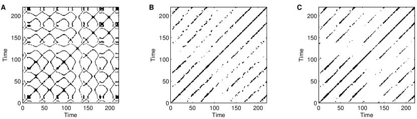
Figure 1: Recurrence plots of the Rössler oscillator with parameters $a=b=0.25$ and $c=40$ using different embedding: (A) $m=1$, $\tau=1$, (B) $m=3$, $\tau=12$, (C) $m=3$, $\tau=6$ (adaptive recurrence threshold to ensure (A) $RR=0.1$, (B, C) $RR=0.05$). Non-optimal embedding can cause line structures perpendicular to the main diagonal, wobbly or interrupted lines (A, B).

3.2 Recurrence threshold selection

The recurrence threshold $\varepsilon$ is a crucial parameter in the RP analysis. Although several works have contributed to this discussion [e.g., Thiel et al., 2002; Matassini et al., 2002; Marwan et al., 2007; Schinkel et al., 2008], a general and systematic study on the recurrence threshold selection remains an open task for future work. Nevertheless, recurrence threshold selection is a trade-off of to have a small threshold as possible but at the same time a sufficient number of recurrences and recurrence structures.

However, the diversity of applicability of RP based methods causes a number of different criteria for the selection of the threshold: studying dynamical properties (dynamical invariants, synchronisation) requires a very small threshold Marwan et al. [2007]; Donner et al. [2010]; twin surrogates or trajectory reconstruction methods may require larger thresholds Hirata et al. [2008]; noise corrupted observation data requires even larger thresholds Thiel et al. [2002]; for studying dynamical transitions, the threshold selection can be even without much importance, because the relative change of the RQA measures does not depend too much on it in a certain range; for the detection of certain signals a specific fraction of the phase space diameter (or standard deviation of the time series) can be required Schinkel et al. [2008].

Several “rules of thumb” for the choice of $\varepsilon$ have been advocated in the literature, e.g., a few per cent of the maximum phase space diameter [Mindlin & Gilmore, 1992], a value that should not exceed 10% of the mean or the maximum phase space diameter [Koebbe & Mayer-Kress, 1992; Zbilut & Webber Jr., 1992], or that the recurrence rate $RR=\sum_{i,j}R_{i,j}/N^{2}$ is approximately 1% Zbilut et al. [2002]. A recently proposed criterion employing the relationship between recurrence rate and $\varepsilon$ defines an optimal value by using the position of the maximum of the first derivative of the recurrence rate $\frac{dRR}{d\varepsilon}$ Gao & Jin [2009]. Such approach can produce ambiguous and highly unstable results, as slight variations in $\varepsilon$ (as possible by minor errors in finding this value or by nonstationary time series) cause high variation in the recurrence structure. Next, the position of the maximum of $\frac{dRR}{d\varepsilon}$ depends strongly on the chosen norm and embedding, and may lead to an overestimation of an optimal $\varepsilon$. And, finally, there are systems which can have more than one maximum Donner et al. [2010].

Another criterion for the choice of $\varepsilon$ takes into account that a measurement of a process is a composition of the real signal and some observational noise with standard deviation $\sigma$ Thiel et al. [2002]. In order to get similar results as for the noise-free situation, $\varepsilon$ has to be chosen such that it is five times larger than the standard deviation of the observational noise, i.e., $\varepsilon>5\,\sigma$. Although this criterion holds for a wide class of processes, it is difficult to estimate the amount of observational noise in the signal.

For (quasi-)periodic processes, it has been suggested to use the diagonal structures within the RP in order to find the optimal $\varepsilon$ Matassini et al. [2002]. In this approach, the density distribution of recurrence points along the diagonals parallel to the LOI is investigated on dependence of $\varepsilon$ in order to minimise the fragmentation and thickness of the diagonal lines with respect to the threshold. However, this choice of $\varepsilon$ may not preserve the important distribution of the diagonal lines in the RP if observational noise is present (the estimated threshold can be underestimated).

The selection of an optimal recurrence threshold $\varepsilon$ is not straightforward and depends on the particular problem and question.

3.3 Indicators of determinism

The length of a diagonal line in the RP corresponds to the time the system evolves very similar as during another time, i.e., a segment of the phase space trajectory runs parallel and within an $\varepsilon$-tube of another segment of the phase space trajectory. Deterministic systems are often characterised by repeated similar state evolution (corresponding to a local predictability), yielding in a large number of diagonal lines in the RP. In contrast, systems with independent subsequent values, like white noise, have RPs with mostly single points. Therefore, the fraction of recurrence points forming such diagonal lines (of length $l\geq l_{\min}$)

$$DET=\frac{\sum_{l\geq l_{\min}}lP(l)}{\sum_{i,j}R_{i,j}}$$ (1)

can be calculated and is, therefore, called determinism in the RQA. Somehow this measure can be interpreted as an indication of determinism in the data. But we should be careful in using the term determinism in a more general or mathematical sense. In a deterministic system we can calculate the same exact state by using given initial conditions, i.e., there is no stochastic process involved. Different methods can be used to test for determinism in time series, e.g., a combined modelling-surrogate approach Small & Tse [2003] or an analysis of the directionality of the phase space trajectory Kaplan & Glass [1992].

High values of $DET$ might be an indication of determinism in the studied system, but it is just a necessary condition, not a sufficient one. Even for non-deterministic processes we can find longer diagonal lines in the RP, resulting in increased $DET$ values. For example, the following (non-deterministic) auto-regressive process $x_{i}=0.8x_{i-1}+0.3x_{i-2}-0.25x_{i-3}+0.9\xi$ (where $\xi$ is white Gaussian noise) has a $DET$ value of 0.6 (embedding dimension $m=4$, delay $\tau=4$, and fixed recurrence rate of 0.1). As it was shown in Thiel et al. [2003], stochastic processes can have RPs containing longer diagonal lines just by chance (although very rare). Moreover, due to embedding we introduce correlations in the RP and, therefore, also uncorrelated data (e.g. from white noise process) have spurious diagonal lines Thiel et al. [2006]; Marwan et al. [2007] (Fig. 2). Moreover, data pre-processing like low-passfiltering (smoothing) is frequently used. Such pre-processing can also introduce spurious line structures in the RP. Therefore, from just a high value of the RQA measure $DET$ we have to be careful in infering that the studied system would be deterministic. For such conclusion we need at least one further criterion included in the RP: the directionality of the trajectory Kaplan & Glass [1992]. One possible solution is to use iso-directional RPs Horai et al. [2002] or perpendicular RPs Choi et al. [1999]; if then the measure reaches $DET\approx 1$ for a very small recurrence density (i.e. $RR<0.05$), the underlying system will be a deterministic one (like a periodic or chaotic system).

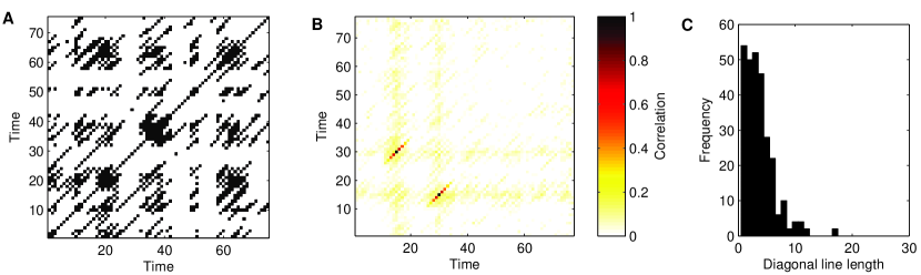
Figure 2: (A) Recurrence plot of one realisation of Gaussian white noise, calculated using embeddeding dimension $m=6$, delay $\tau=1$, and a recurrence threshold of $\varepsilon=0.2$. The embedding causes a number of long lines. (B) Correlation between a single recurrence point at $(15,30)$ and other recurrence points in the RP of white noise demonstrating the effect of embedding for a bogusly creation of long diagonal lines (estimated from 1,000 realisations). (C) The histogram of line lengths found in the RP shown in (A). The maximum length is $L_{\max}=17$, a value, which would not be uncommon for a deterministic process.

3.4 Indicators of periodic systems

As explained in the previous section, deterministic systems cause a high value in the RQA measure $DET$. This measure has been successfully used to detect transitions in the dynamics of complex systems Trulla et al. [1996]. A frequently used example in order to present this ability is the study of the different dynamical regimes of the logistic map, where $DET$ is able to detect the periodic windows (by values $DET=1$). Therefore, it is often claimed that this measure is able to detect chaos-period transitions.

However, we can also find such high $DET$ values for non-periodic, but chaotic systems. For example, the Rössler system Rössler [1976],

$$\left(\frac{dx}{dt},\,\frac{dy}{dt},\,\frac{dz}{dt}\right)=\bigl{(}-y-z,\ x+0.25y,\ 0.25+z(x-c)\bigr{)},$$ (2)

exhibits in the parameter interval $c\in[35,\,45]$ a transition from periodic to chaotic states (Fig. 3A). But due to the smooth phase space trajectory and high sampling frequency (sampling time $\Delta t=0.1$), the RP for the chaotic trajectory consists almost exclusively on diagonal line structures (Fig. 4), resulting in a high value of $DET$, i.e., $DET\approx 1$ (Fig. 3B).

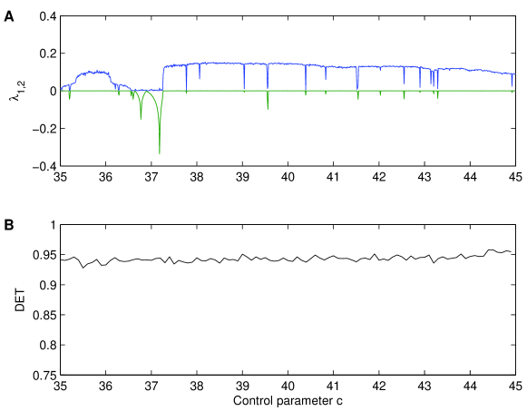
Figure 3: (A) 1st and 2nd positive Lyapunov exponents of the Rössler oscillator with parameters $a=b=0.25$ and $c\in[35,\,45]$. A periodic window occurs between $c=36.56$ and $c=37.25$. However, the $DET$ measures reveals an almost constant very high value of approximately $DET=0.94$. Used RP parameters: dimension $m=3$, delay $\tau=6$, adaptive recurrence threshold to ensure a $RR=0.05$.

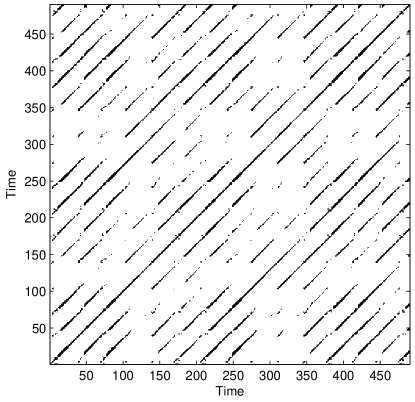
Figure 4: Recurrence plot of the Rössler oscillator with parameters $a=b=0.25$ and $c=40$. For this parameters, the Rössler system is in a chaotic regime ($\lambda_{1}=0.14$), but the RP consists almost only on diagonal lines. Used RP parameters: dimension $m=3$, delay $\tau=6$, adaptive recurrence threshold to ensure a $RR=0.05$.

A very high value of $DET$ is not a clear or even sufficient indication of a periodic system. High values can be caused by very smooth phase space trajectories. This should also be considered when looking for indications of unstable periodic orbits (UPOs), where $DET$ or mean and maximal line lengths $L$ and $L_{\max}$ may not be sufficient. A solution could be to increase the minimal length $l_{\min}$ of a diagonal recurrence structure which is considered to be a line. However, a better solution is to look at the cumulative distribution of the diagonal line lengths and estimate the $K_{2}$ entropy (but this requires much longer time series, cf. Subsect. 3.9). Recent work has shown that measures coming from complex network theory, like clustering coefficient, applied to recurrence matrices are more powerful and reliable for the detection of periodic dynamics Marwan et al. [2009]; Zou et al. [subm.]; Donner et al. [XXXX].

3.5 Indicators of chaos

The RP visualises the recurrence structure of the considered system (based on the phase space trajectory). The basic idea behind RPs comes, in general, from the study of chaos. Therefore it can be considered as a nonlinear tool for data analysis. But this cannot be a criterion to understand complex structures in the RP or high values of RQA measures as indicators of chaos or nonlinearity in the dynamical system.

As mentioned above, uncorrelated stochastic systems have mostly short or almost no diagonal line structures in their RPs, whereas deterministic and regular systems, like periodic processes, have mostly long and continuous diagonal line structures. Chaotic processes have also diagonal, but shorter lines, and can have single recurrence points. Nevertheless, only by looking at the appearance of an RP it is difficult (almost impossible) to infer about the type of dynamics; only periodic and white noise processes can be identified with some certainty.

The alternative is to look at the RQA measures quantifying the structures in an RP which are related to some dynamical characteristics of the system. As diagonal lines in the RP correspond to parallel running trajectory segments, it is clear that the length of these lines is somehow related to the divergence behaviour of the dynamical system. Divergence rate of phase space trajectories is measured by the Lyapunov exponent. In fact, the lengths of the diagonal lines are directly related to dynamical invariants as $K_{2}$ entropy or $D_{2}$ correlation dimension Faure & Korn [1998]; Thiel et al. [2004]. The $K_{2}$ entropy is the lower limit of the sum of the positive Lyapunov exponents.

For example, RQA measures based on the length of the diagonal lines, like determinism $DET$ and mean line length $L$, also depend on the type of the dynamics of the systems (rather low values for uncorrelated stochastic (white noise) systems, higher values for more regular, correlated and also chaotic systems). It has been suggested to measure the length of the longest diagonal line $L_{\max}$ and interpret its inverse $DIV=1/L_{\max}$ as an estimator of the maximal Lyapunov exponent Trulla et al. [1996]. However, this interpretation incorporates high potential of erroneous conclusions derived from RQA.

First, the main diagonal in the RP (i.e., the line of identity, LOI) is naturally the longest diagonal line, wherefore it is usually excluded from the analysis. However, due to the tangential motion of the phase space trajectory, subsequent phase space vectors are often also considered as recurrence points (known as sojourn points) Marwan et al. [2007]. These recurrence points lead to further continuous diagonal lines directly close to the LOI. Without excluding an appropriate corridor along the LOI (the Theiler window), $L_{\max}$ will be artificially large ($\approx N$) and $DIV$ too small.

Second, as explained above, even white noise can have long diagonal lines Thiel et al. [2003], leading to a small $DIV$ value just by chance (Fig. 2). Although the probability for the occurrence of such long lines is rather small, the probability that lines of length two occur in RPs of stochastic processes is, on the contrary, rather high. Only one line of length two is enough to get a finite value of $DIV$ which might be mis-interpreted as a finite Lyapunov exponent and that the system would be chaotic instead stochastic.

Therefore, we have to be careful in interpreting the RQA measures themselves as indicators of chaos. Moreover, such conclusion cannot be drawn by applying a simple surrogate test where the data points are simply shuffled (such a test would only destroy the correlation structure within the data, and, thus, the frequency information).

RP or RQA alone cannot be used to infer nonlinearity from a time series. For this purpose, advanced surrogate techniques are more appropriate Schreiber & Schmitz [2000]; Rapp et al. [2001].

3.6 Discrimination analysis and detection of deterministic signals

RQA is also a powerful tool in order to distinguish between different types of signals, different groups of dynamical regimes etc. [e.g., Zbilut et al., 1998; Marwan et al., 2002b; Facchini et al., 2007; Litak et al., 2010]. However, the selection of applicable RQA measures is a crucial task. Not all measures will be useful for all questions. Their application needs justification in terms of the purpose of the intended analysis. For example, for processes which does not contain laminar regimes, or if we are not interested in the detection of such laminar regimes, it would not make sense to use RQA measures basing on vertical recurrence structures (like laminarity or trapping time) Marwan & Kurths [2009].

3.7 Indicators of nonstationarity and transition analysis

RQA is powerful for the analysis of slight changes and transitions in the dynamics of a complex system. For this purpose we need a time-dependend RQA (a RQA series) what can be realised in two ways (Fig. 5):

(1) The RP is covered with small overlapping windows of size $w$ spreading along the LOI and in which the RQA will be calculated, $R_{i,j}|_{i,j=k}^{k+w-1}$.

(2) The time series (or phase space trajectory) is divided into overlapping segments $x_{i}|_{i=k}^{k+w-1}$ from which RPs and subsequent RQA will be calculated separately.

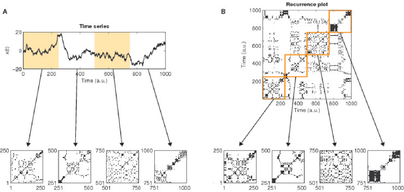
Figure 5: Two possibilities of windowed RQA: (A) Windowing of time series and (B) windowing of RP. The example is an auto-regressive process: $x_{i}=0.95x_{i-1}+0.05x_{i-2}+0.9\xi$ (where $\xi$ is white Gaussian noise), the RP is calculated using a constant number of neighbours (10% of all points) and without embedding. The sub-RPs at the bottom clearly demonstrate the differences between the two approaches.

Such time dependent approach can also be used to analyse the stationarity of the dynamical system.

Here we should note the following important points. The time scale of the RQA values depends on the choice which point in the window should be considered as the corresponding time point. Selecting the first point $k$ of the window as the time point of the RQA measures allows to directly transfer the time scale of the time series to the RQA series. However, the window reaches into the future of the current time point and, thus, the RQA measures represent a state which lies in the future. Variations in the RQA measures can be misinterpreted as early signs of later state transitions (like a prediction). A better choice is therefore to select the centre of the window as the current time point of the RQA. Then the RQA considers states in the past and in the future. If strict causality is required (crucial when attempting to detect subtle changes in the dynamics just prior the onset of dramatic state changes), it might be even useful to select the end point of the window as the current time point of the RQA (using embedding we have to add $(m-1)\tau-1$). For most applications the centre point should be appropriate.

Another important issue can rise from the different windowing methods (1) or (2), which are only equivalent when we do not normalise the time series (or its pieces) from which the RP is calculated and when we chose a fixed threshold recurrence criterion. If we normalise the time series just before the RP calculation, we get differently normalised segments resulting in different sub-RPs (and thus different RQA results) than such derived directly by moving windows from the RP of the entire time series (Fig. 5 and Tab. 3.7). A similar problem arises when we use a fixed number of nearest neighbours for the definition of recurrence, because it is a big difference considering the entire time series in order to find the $k$ nearest neighbours or just a small piece of it. Nevertheless, both approaches (1) and (2) can be useful and depend on the given question. If we know that the time series shows some nonstationarities or trends which are not of interest, then approach (2) can help to find transitions neglecting these nonstationarities. But, if we are interested in the detection of the overall changes (e.g., to test for nonstationarity), we should keep the numerical conditions for the entire available time constant and chose approach (1). Anyway, for each RQA we should explicitly state how the windowing procedure has been performed.

Selected RQA measures derived from windowing of time series (left) and windowing of RP (right) of an auto-regressive process and windowing as shown in Fig. 5. Window 1–250 251–500 501–750 751–1000 $RR$ 0.10 0.10 0.10 0.10 $DET$ 0.62 0.74 0.48 0.79 $L$ 3.13 3.69 2.75 3.75   Window 1–250 251–500 501–750 751–1000 $RR$ 0.18 0.12 0.20 0.19 $DET$ 0.81 0.81 0.69 0.95 $L$ 3.78 4.27 2.90 9.50

The choice of the window size itself needs the same attention. Because the RQA measures are statistical measures derived from histograms, the window should be large enough to cover a sufficient number of recurrence lines or orbits. A too small window can pretend strong fluctuations in the RQA measures just by weak statistical significance (the RQA measure $TREND$ is very sensitive to the window size and can reveal even contrary results, cp. Fig. 7B). Therefore, conclusions about nonstationarity of the system should be drawn with much care. Moreover, statements on stationarity of the system itself are questionable at all (if not enough knowledge about the system is available), because detected nonstationarity in an observed finite time series does not mean automatically nonstationarity in the underlying system. For example, an auto-regressive process is stationary by definition, but its RP and RQA can reveal a nonstationary signal (Figs. 6 and 7).

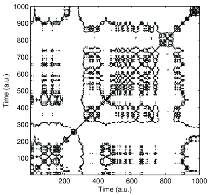
Figure 6: RP of the same auto-regressive process as presented in Fig. 5, which is by definition stationary. The RP is calculated using maximum norm, $\varepsilon=2$ and without embedding.

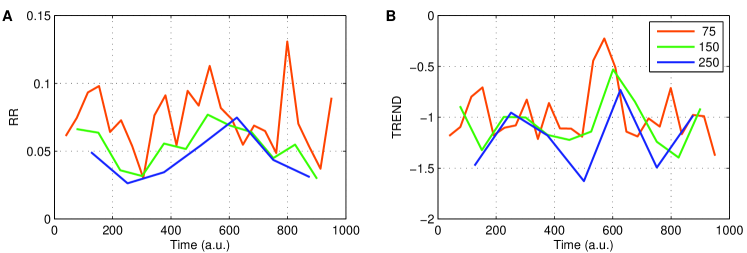
Figure 7: Two exemplary RQA measures, (A) recurrence rate $RR$ and (B) paling trend ($TREND$), of the auto-regressive process as presented in Fig. 5 for three different window sizes $w$ ($w=75,150,250$). (A) The strong variation in $RR$ pretends a nonstationarity in the signal. (B) $TREND$ depends rather strongly on $w$, resulting in contrary outcomes, e.g., revealing high values for $w=250$, but small values for $w=75$ at the same time period $t=700\ldots 800$. The RQA is calculated using maximum norm, $\varepsilon=0.3$ and without embedding (the windows are moved by $w/2$, i.e., 50% overlap; the RQA time point is set to the centre of the RQA window).

3.8 Significance of RQA measures

Related to the preceding issue on windowed RQA is the question on the significance of the RQA variation. A sub-optimal scaling of the variation of the RQA measures can mislead to conclusions that the studied system has changed its regime or that it would be nonstationary (Fig. 8A, B). Therefore, it is strongly recommended to cross-check the scaling of the presentation and to present confidence intervals (Fig. 8C, D). Confidence intervals can be calculated in various ways, but we should avoid to derive them by simply shuffling the original data. One approach could be a bootstrap resampling of the line structures in the RP Marwan et al. [2008]; Schinkel et al. [2009]. Another approach fits the probability of serial dependences (diagonal lines) to a binomial distribution Hirata & Aihara [XXXX]. Whatever approach we chose, the estimation of the confidence intervals is not a trivial task, but in the future the standard software for RQA should include such tests.

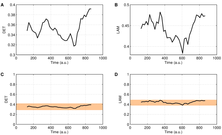
Figure 8: Two exemplary RQA measures, (A, C) determinism $DET$ and (B, D) laminarity ($LAM$), of the auto-regressive process as presented in Fig. 5. (A, B) The scaling of the $y$-axis is affecting a strong variation in the RQA measures – a potential of wrong conclusions. (C, D) Considering a 5% confidence interval of the RQA measures (details can be found in Marwan et al. [2008]) and a better value range for the $y$-axis, we cannot infer that the values of the RQA measures as shown in (A) and (B) significantly vary. The RQA is calculated using a window size of $w=250$ and a window step of $ws=20$, using maximum norm, $\varepsilon=0.3$ and without embedding (the RQA time point is set to the centre of the RQA window). $LAM$ is the fraction of recurrence points forming vertical lines in an RP (analogously as $DET$ for the diagonal lines).

A common statement on recurrence analysis is that it is useful to analyse short data series. But we have to ask, how short is short? The required length for the estimation of dynamical invariants will be discussed in the following Subsect. Applying RQA analysis we should be aware that the RQA measures are statistical measures (like an average) and need some minimal length that a variation can be considered to be significant.

3.9 Dynamical invariants from short time series

An RP analysis is appropriate for analysing short and nonstationary time series, as it is often stated in many reports Fabretti & Ausloos [2005]; Schinkel et al. [2007]; Zbilut et al. [1998]. However, this statement holds actually only for the heuristic measures of complexity as introduced for the RQA or for the detection of differences or transitions in data series. If we are interested in the dynamical invariants derived from RPs, the length $N$ of the time series becomes a more crucial part like it is for the standard methods of nonlinear data analysis.

The derivations of dimensions ($D_{1}$, $D_{2}$) and dynamical invariants (like $K_{2}$) from the RPs hold only in the limit $N\rightarrow\infty$ and small $\varepsilon$ ($\varepsilon\rightarrow 0$). Nevertheless, an estimation of dynamical invariants from shorter time series can be feasible. We have to regard the following factors if discussing the time series length: the number of orbits representing stretching, the number of recurrences filling out a sufficient part of the attractor, and the number of data points necessary for an acceptable phase space reconstruction Wolf et al. [1985]. Since these factors may require different minimal lengths, the largest of these lengths should be considered.

For example, numerical considerations for the estimation of the attractor (correlation) dimension $D_{2}$ using the Grassberger-Procaccia algorithm Grassberger & Procaccia [1983] lead to the requirement $\log N>\frac{D_{2}}{2}\log(\frac{1}{\varrho})$ (where $\varrho=\frac{S}{\varepsilon}$ is the fraction the recurrence neighbourhood of size $\varepsilon$ covers on the entire phase space of diameter $S$) Eckmann & Ruelle [1998]. Considering a $\varrho=0.1$ and a decimal logarithm, for finding a $D_{2}=10$ we need at least $N=100,000$ data points. Furthermore, a $\varrho=0.1$ is actually too large and we need much smaller $\varepsilon$, which consequently provokes that again a larger $N$ is required.

For Lyapunov exponents (and analogously for $K_{2}$), a rough estimate based on the mentioned requirements suggests minimal time series lengths of $10^{D_{2}}$ to $30^{D_{2}}$ (with attractor dimension $D_{2}$) Wolf et al. [1985]. Accordingly, a system with $D_{2}=3$ requires 1000–30,000 data points (a more strict consideration even requires $\log N>D_{2}\log(\frac{1}{\varrho})$ Eckmann & Ruelle [1998]).

Therefore, too guarantee useful results we need long time series. If we calculate dimensions or $K_{2}$ from short time series the results are probably worthless.

3.10 Synchronisation and line of synchronisation

Cross recurrence plots (CRPs) can be used for the investigation of the simultaneous evolution of two different phase space trajectories Marwan et al. [2002a]; Marwan & Kurths [2002]; Zolotova et al. [2009]; Ihrke et al. [2009]. The line of identity (LOI) in the RP becomes a line of synchronisation (LOS) in the CRP. Two more-or-less identical systems but with differences on the time-scale will reveal a bowed LOS Marwan et al. [2002a]; Marwan & Kurths [2005]. An off-set of the LOS away from the main diagonal is an indication of a phase shift or a delay between the two considered systems.

However, because this method tests if the two trajectories visit the same region in the phase space, it can be used only to study complete synchronisation (CS) or a kind of a generalised correlation (although with possible delays), or to get the relation between the transformations between their time-scales. Moreover, the data under consideration should be from the same (or a very comparable) process and, actually, should represent the same observable. Therefore, the reconstructed phase space should be the same.

For the study of the LOS the distance matrix may be more appropriate because it contains more information, especially if the data series show nonstationarities. Then, the LOS can be found by using efficient algorithms like dynamic time warping Sakoe & Chiba [1978]. Nevertheless, it is always very important to check if the found LOS makes sense; for instance, it is possible to find several LOS (cp. Application in magneto-stratigraphy in Marwan et al. [2007]).

3.11 Macrostructures and sampling

For the visual interpretation of an RP and also for a reliable RQA we should remember that our data are discretised time or data series. The sampling of the signal has an importance which should not be underestimated. If the sampling frequency is just one magnitude higher than the system’s main frequencies, and their ratio is not a multiple of an integer (i.e., we have an intrinsic phase error), an interference triggered by the sampling of the continuous signal can produce large empty regions in the recurrence matrix, although they should be there Facchini et al. [2005]; Facchini & Kantz [2007]. Nonstationarities or modulations in frequency or phase cause non-trivial gaps or macrostructures in the recurrence matrix (Fig. 9). We should be aware that such gaps can occur in particular when we use a low sampling frequency. The recurrence structure of interest can appear rather different; diagonal lines can vanish or can be reduced to just single points yielding in biased RQA measures (Fig. 10).

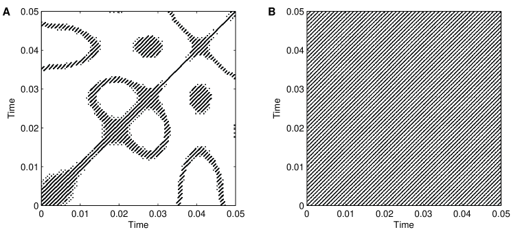
Figure 9: RP of a modulated harmonic oscillation $\sin(2\pi 1000(\pi+t)+2\pi\sin(2\pi 44t)t)$. (A) Non-trivial macrostructures (gaps) in the RP due to the interference of the sampling frequency of 1 kHz and the frequency of the modulated harmonic signal. (B) Corresponding RP as shown in (A), but for a higher sampling frequency of 10 kHz. As expected, the entire RP now consists of the periodic line structures due to the oscillation. Used RP parameters: dimension $m=3$, delay $\tau=1$, recurrence threshold $\varepsilon=0.05\sigma$, $L_{\infty}$-norm.

Nevertheless, tiny modulations in frequency or phase in oscillating signals can be detected by RPs, which are non-detectable by standard methods (spectral or wavelet analysis). This turns RPs to a powerful tool for the analysis of slight modulations in oscillatory signals like audio signals.

Please note that macrostructures are also an apparent problem when displaying large RPs on a computer screen (and up to a certain amount on print outs). The resolution of modern computer screens is around 72 ppi (points per inch, 72 ppi corresponds to around 28 points per centimetre). The presentation of RPs in a window of, e.g., 6 inch allows only the display of around 430 points. Larger RPs will be rendered using downsampling or interpolation, resulting in similar interference effects and artificial secondary macrostructures as described above; such macrostructures will even change for different window sizes (Fig. 11). Therefore, we should take care in visual interpretation of patterns found in large RPs which are represented on computer screens.

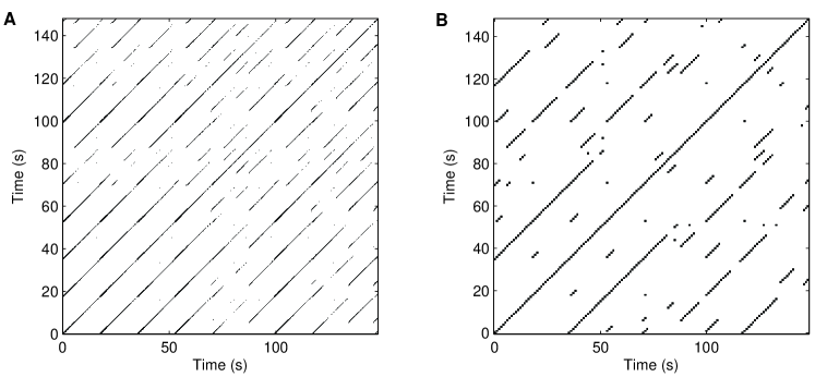
Figure 10: RP of the $x$-component of the Rössler oscillator, Eq. (2), with parameters $a=b=0.2,c=5.7$. The sampling time is (A) $\Delta t=0.05$ and (B) $\Delta t=1$. The embedding was chosen in both settings to be equivalent: dimension in (A) and (B) is $m=3$, the delay in (A) $\tau=20$, but in (B) $\tau=1$; recurrence threshold $\varepsilon=1.5$ (maximum norm). Due to the low sampling in (B), many diagonal lines vanish.

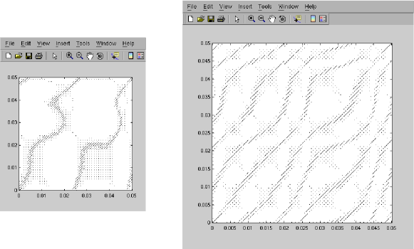
Figure 11: Screenshot of the RP as shown in Fig. 9B for two different window sizes of display on a computer screen (using Matlab^®). Although the RP consists only on continuous diagonal lines as represented in Fig. 9B, its size ($N=5511$) exceeds the screen resolution and requires downsampling, leading to artifical macrostructures.

4 Conclusions

We have illustrated several problems regarding the application of recurrence plots (RPs) and recurrence quantification analysis (RQA) which need our attention in order to avoid wrong results. The uncritical application of these methods can yield to serious pitfalls. Therefore, it is important to understand the basic principles and ideas behind the measures of complexity forming the RQA and the different techniques to study the numerous phenomena of complex systems, like transitions, synchronisation, etc. Nevertheless, the recurrence plot based techniques are still a rather young field in nonlinear time series analysis, and many open questions remain. For example, systematic research is necessary to define reliable criteria for the selection of the recurrence threshold, and the estimation of the confidence of the RQA measures will be a hot topic in the near future.

Acknowledgments The work has been supported by the Potsdam Research Cluster for Georisk Analysis, Environmental Change and Sustainability (PROGRESS).

References

- Belaire-Franch [2004] Belaire-Franch, J. [2004] “Testing for non-linearity in an artificial financial market: a recurrence quantification approach,” Journal of Economic Behavior & Organization 54, 483–494, 10.1016/j.jebo.2003.05.001.
- Čermák [2009] Čermák, V. [2009] “Recurrence Quantification Analysis of Borehole Temperatures: Evidence of Fluid Convection,” International Journal of Bifurcation and Chaos 19, 889–902, 10.1142/S0218127409023366.
- Choi et al. [1999] Choi, J. M., Bae, B. H. & Kim, S. Y. [1999] “Divergence in perpendicular recurrence plot; quantification of dynamical divergence from short chaotic time series,” Physics Letters A 263, 299–306, 10.1016/S0375-9601(99)00751-3.
- Donner et al. [XXXX] Donner, R. V., Small, M., Donges, J. F., Marwan, N., Zou, Y. & Kurths, J. [XXXX] “Recurrence-based time series analysis by means of complex network methods,” International Journal of Bifurcation and Chaos (this special issue).
- Donner et al. [2010] Donner, R. V., Zou, Y., Donges, J. F., Marwan, N. & Kurths, J. [2010] “Ambiguities in recurrence-based complex network representations of time series,” Physical Review E 81, 015101(R), 10.1103/PhysRevE.81.015101.
- Eckmann et al. [1987] Eckmann, J.-P., Oliffson Kamphorst, S. & Ruelle, D. [1987] “Recurrence Plots of Dynamical Systems,” Europhysics Letters 5, 973–977.
- Eckmann & Ruelle [1998] Eckmann, J.-P. & Ruelle, D. [1998] “Fundamental limitations for estimating dimensions and Lyapunov exponents in dynamical systems,” Physica D 56, 185–187, 10.1016/0167-2789(92)90023-G.
- Fabretti & Ausloos [2005] Fabretti, A. & Ausloos, M. [2005] “Recurrence plot and recurrence quantification analysis techniques for detecting a critical regime. Examples from financial market indices,” International Journal of Modern Physics C 16, 671–706, 10.1142/S0129183105007492.
- Facchini & Kantz [2007] Facchini, A. & Kantz, H. [2007] “Curved structures in recurrence plots: The role of the sampling time,” Physical Review E 75, 036215, 10.1103/PhysRevE.75.036215.
- Facchini et al. [2005] Facchini, A., Kantz, H. & Tiezzi, E. B. P. [2005] “Recurrence plot analysis of nonstationary data: The understanding of curved patterns,” Physical Review E 72, 021915, 10.1103/PhysRevE.72.021915.
- Facchini et al. [2007] Facchini, A., Mocenni, C., Marwan, N., Vicino, A. & Tiezzi, E. B. P. [2007] “Nonlinear time series analysis of dissolved oxygen in the Orbetello Lagoon (Italy),” Ecological Modelling 203, 339–348, 10.1016/j.ecolmodel.2006.12.001.
- Faure & Korn [1998] Faure, P. & Korn, H. [1998] “A new method to estimate the Kolmogorov entropy from recurrence plots: its application to neuronal signals,” Physica D 122, 265–279, 10.1016/S0167-2789(98)00177-8.
- Gao & Jin [2009] Gao, Z. & Jin, N. [2009] “Flow-pattern identification and nonlinear dynamics of gas-liquid two-phase flow in complex networks,” Physical Review E 79, 066303, 10.1103/PhysRevE.79.066303.
- Grassberger & Procaccia [1983] Grassberger, P. & Procaccia, I. [1983] “Characterization of strange attractors,” Physical Review Letters 50, 346–349, 10.1103/PhysRevLett.50.346.
- Groth [2005] Groth, A. [2005] “Visualization of coupling in time series by order recurrence plots,” Physical Review E 72, 046220, 10.1103/PhysRevE.72.046220.
- Hirata & Aihara [XXXX] Hirata, Y. & Aihara, K. [XXXX] “Statistical tests for serial dependence and laminarity on recurrence plots,” International Journal of Bifurcation and Chaos (this special issue).
- Hirata et al. [2008] Hirata, Y., Horai, S. & Aihara, K. [2008] “Reproduction of distance matrices from recurrence plots and its applications,” European Physical Journal – Special Topics 164, 13–22, 10.1140/ep jst/e2008-00830-8.
- Horai et al. [2002] Horai, S., Yamada, T. & Aihara, K. [2002] “Determinism Analysis with Iso-Directional Recurrence Plots,” IEEE Transactions - Institute of Electrical Engineers of Japan C 122, 141–147.
- Ihrke et al. [2009] Ihrke, M., Schrobsdorff, H. & Herrmann, J. M. [2009] “Recurrence-Based Synchronization of Single Trials for EEG-Data Analysis,” Lecture Notes in Computer Science: Intelligent Data Engineering and Automated Learning – IDEAL 2009 5788, 118–125, 10.1007/978-3-642-04394-9.
- Kantz & Schreiber [1997] Kantz, H. & Schreiber, T. [1997] Nonlinear Time Series Analysis (University Press, Cambridge).
- Kaplan & Glass [1992] Kaplan, D. T. & Glass, L. [1992] “Direct test for determinism in a time series,” Physical Review Letters 68, 427–430.
- Koebbe & Mayer-Kress [1992] Koebbe, M. & Mayer-Kress, G. [1992] “Use of Recurrence Plots in the Analysis of Time-Series Data,” Proceedings of SFI Studies in the Science of Complexity, eds. Casdagli, M. & Eubank, S. (Addison-Wesley, Redwood City), pp. 361–378.
- Komalapriya et al. [2010] Komalapriya, C., Romano, M. C., Thiel, M., Marwan, N., Kurths, J., Kiss, I. Z. & Hudson, J. L. [2010] “An automated algorithm for the generation of dynamically reconstructed trajectories,” Chaos 20, 013107, 10.1063/1.3279680.
- Litak et al. [2010] Litak, G., Wiercigroch, M., Horton, B. W. & Xu, X. [2010] “Transient chaotic behaviour versus periodic motion of a parametric pendulum by recurrence plots,” ZAMM – Journal of Applied Mathematics and Mechanics/ Zeitschrift f r Angewandte Mathematik und Mechanik 90, 33–41, 10.1002/zamm.200900290.
- Mandelbrot [1982] Mandelbrot, B. B. [1982] The fractal geometry of nature (Freeman, San Francisco).
- Marwan [2008] Marwan, N. [2008] “A Historical Review of Recurrence Plots,” European Physical Journal – Special Topics 164, 3–12, 10.1140/epjst/e2008-00829-1.
- Marwan et al. [2009] Marwan, N., Donges, J. F., Zou, Y., Donner, R. V. & Kurths, J. [2009] “Complex network approach for recurrence analysis of time series,” Physics Letters A 373, 4246–4254, 10.1016/j.physleta.2009.09.042.
- Marwan & Kurths [2002] Marwan, N. & Kurths, J. [2002] “Nonlinear analysis of bivariate data with cross recurrence plots,” Physics Letters A 302, 299–307, 10.1016/S0375-9601(02)01170-2.
- Marwan & Kurths [2005] Marwan, N. & Kurths, J. [2005] “Line structures in recurrence plots,” Physics Letters A 336, 349–357, 10.1016/j.physleta.2004.12.056.
- Marwan & Kurths [2009] Marwan, N. & Kurths, J. [2009] “Comment on “Stochastic analysis of recurrence plots with applications to the detection of deterministic signals” by Rohde et al. [Physica D 237 (2008) 619–629],” Physica D 238, 1711–1715, 10.1016/j.physd.2009.04.018.
- Marwan et al. [2007] Marwan, N., Romano, M. C., Thiel, M. & Kurths, J. [2007] “Recurrence Plots for the Analysis of Complex Systems,” Physics Reports 438, 237–329, 10.1016/j.physrep.2006.11.001.
- Marwan et al. [2008] Marwan, N., Schinkel, S. & Kurths, J. [2008] “Significance for a recurrence based transition analysis,” Proceedings of the International Symposium on Nonlinear Theory and its Applications (NOLTA2008), Budapest (Budapest, Hungary), pp. 412–415.
- Marwan et al. [2002a] Marwan, N., Thiel, M. & Nowaczyk, N. R. [2002a] “Cross Recurrence Plot Based Synchronization of Time Series,” Nonlinear Processes in Geophysics 9, 325–331.
- Marwan et al. [2002b] Marwan, N., Wessel, N., Meyerfeldt, U., Schirdewan, A. & Kurths, J. [2002b] “Recurrence Plot Based Measures of Complexity and its Application to Heart Rate Variability Data,” Physical Review E 66, 026702, 10.1103/PhysRevE.66.026702.
- Matassini et al. [2002] Matassini, L., Kantz, H., Hołyst, J. A. & Hegger, R. [2002] “Optimizing of recurrence plots for noise reduction,” Physical Review E 65, 021102, 10.1103/PhysRevE.65.021102.
- Mindlin & Gilmore [1992] Mindlin, G. M. & Gilmore, R. [1992] “Topological analysis and synthesis of chaotic time series,” Physica D 58, 229–242, 10.1016/0167-2789(92)90111-Y.
- Packard et al. [1980] Packard, N. H., Crutchfield, J. P., Farmer, J. D. & Shaw, R. S. [1980] “Geometry from a Time Series,” Physical Review Letters 45, 712–716, 10.1103/PhysRevLett.45.712.
- Pecar [2003] Pecar, B. [2003] “The use of Visual Recurrence Analysis and Hurst exponents as qualitative tools for analysing financial time series,” .
- Rapp et al. [2001] Rapp, P. E., Cellucci, C. J., Korslund, K. E., Watanabe, T. A. & Jimenez-Montano, M. A. [2001] “Effective normalization of complexity measurements for epoch length and sampling frequency,” Physical Review E 64, 16209, 10.1103/PhysRevE.64.016209.
- Romano et al. [2005] Romano, M. C., Thiel, M., Kurths, J., Kiss, I. Z. & Hudson, J. [2005] “Detection of synchronization for non-phase-coherent and non-stationary data,” Europhysics Letters 71, 466–472, 10.1209/epl/i2005-10095-1.
- Rössler [1976] Rössler, O. E. [1976] “An equation for continuous chaos,” Physics Letters A 57, 397–398, 10.1016/0375-9601(76)90101-8.
- Sakoe & Chiba [1978] Sakoe, H. & Chiba, S. [1978] “Dynamic Programming Algorithm Optimization for Spoken Word Recognition,” IEEE Transactions on Acoustics, Speech and Signal Processing ASSP-26, 43–49.
- Schinkel et al. [2008] Schinkel, S., Dimigen, O. & Marwan, N. [2008] “Selection of recurrence threshold for signal detection,” European Physical Journal – Special Topics 164, 45–53, 10.1140/epjst/e2008-00833-5.
- Schinkel et al. [2009] Schinkel, S., Marwan, N., Dimigen, O. & Kurths, J. [2009] “Confidence bounds of recurrence-based complexity measures,” Physics Letters A 373, 2245–2250, 10.1016/j.physleta.2009.04.045.
- Schinkel et al. [2007] Schinkel, S., Marwan, N. & Kurths, J. [2007] “Order patterns recurrence plots in the anaylsis of ERP data,” Cognitive Neurodynamics 1, 317–325, 10.1007/s11571-007-9023-z.
- Schreiber & Schmitz [2000] Schreiber, T. & Schmitz, A. [2000] “Surrogate time series,” Physica D 142, 346–382, 10.1016/S0167-2789(00)00043-9.
- Senthilkumar et al. [2006] Senthilkumar, D. V., Lakshmanan, M. & Kurths, J. [2006] “Phase synchronization in time-delay systems,” Physical Review E 74, 035205, 10.1103/PhysRevE.74.035205.
- Small & Tse [2003] Small, M. & Tse, C. K. [2003] “Detecting Determinism in Time Series: The Method of Surrogate Data,” IEEE Transactions on Circuits and Systems: Fundamental Theory and Applications 50, 663–672.
- Thiel et al. [2003] Thiel, M., Romano, M. C. & Kurths, J. [2003] “Analytical Description of Recurrence Plots of white noise and chaotic processes,” Izvestija vyssich ucebnych zavedenij/ Prikladnaja nelinejnaja dinamika – Applied Nonlinear Dynamics 11, 20–30.
- Thiel et al. [2006] Thiel, M., Romano, M. C. & Kurths, J. [2006] “Spurious Structures in Recurrence Plots Induced by Embedding,” Nonlinear Dynamics 44, 299–305, 10.1007/s11071-006-2010-9.
- Thiel et al. [2002] Thiel, M., Romano, M. C., Kurths, J., Meucci, R., Allaria, E. & Arecchi, F. T. [2002] “Influence of observational noise on the recurrence quantification analysis,” Physica D 171, 138–152, 10.1016/S0167-2789(02)00586-9.
- Thiel et al. [2008] Thiel, M., Romano, M. C., Kurths, J., Rolfs, M. & Kliegl, R. [2008] “Generating surrogates from recurrences,” Philosophical Transactions of the Royal Society A 366, 545–557, 10.1098/rsta.2007.2109.
- Thiel et al. [2004] Thiel, M., Romano, M. C., Read, P. L. & Kurths, J. [2004] “Estimation of dynamical invariants without embedding by recurrence plots,” Chaos 14, 234–243, 10.1063/1.1667633.
- Trauth et al. [2003] Trauth, M. H., Bookhagen, B., Marwan, N. & Strecker, M. R. [2003] “Multiple landslide clusters record Quaternary climate changes in the northwestern Argentine Andes,” Palaeogeography Palaeoclimatology Palaeoecology 194, 109–121, 10.1016/S0031-0182(03)00273-6.
- Trulla et al. [1996] Trulla, L. L., Giuliani, A., Zbilut, J. P. & Webber Jr., C. L. [1996] “Recurrence quantification analysis of the logistic equation with transients,” Physics Letters A 223, 255–260, 10.1016/S0375-9601(96)00741-4.
- Webber Jr. & Zbilut [1994] Webber Jr., C. L. & Zbilut, J. P. [1994] “Dynamical assessment of physiological systems and states using recurrence plot strategies,” Journal of Applied Physiology 76, 965–973.
- Wolf et al. [1985] Wolf, A., Swift, J. B., Swinney, H. L. & Vastano, J. A. [1985] “Determining Lyapunov Exponents from a Time Series,” Physica D 16, 285–317, 10.1016/0167-2789(85)90011-9.
- Zbilut et al. [2004] Zbilut, J. P., Giuliani, A., Colosimo, A., Mitchell, J. C., Colafranceschi, M., Marwan, N., Uversky, V. N. & Webber Jr., C. L. [2004] “Charge and Hydrophobicity Patterning along the Sequence Predicts the Folding Mechanism and Aggregation of Proteins: A Computational Approach,” Journal of Proteome Research 3, 1243–1253, 10.1021/pr049883+.
- Zbilut et al. [1998] Zbilut, J. P., Giuliani, A. & Webber Jr., C. L. [1998] “Detecting deterministic signals in exceptionally noisy environments using cross-recurrence quantification,” Physics Letters A 246, 122–128, 10.1016/S0375-9601(98)00457-5.
- Zbilut & Webber Jr. [1992] Zbilut, J. P. & Webber Jr., C. L. [1992] “Embeddings and delays as derived from quantification of recurrence plots,” Physics Letters A 171, 199–203, 10.1016/0375-9601(92)90426-M.
- Zbilut et al. [2002] Zbilut, J. P., Zaldívar-Comenges, J.-M. & Strozzi, F. [2002] “Recurrence quantification based Liapunov exponents for monitoring divergence in experimental data,” Physics Letters A 297, 173–181, 10.1016/S0375-9601(02)00436-X.
- Zolotova et al. [2009] Zolotova, N. V., Ponyavin, D. I., Marwan, N. & Kurths, J. [2009] “Long-term asymmetry in the wings of the butterfly diagram,” Astronomy & Astrophysics 505, 197–201, 10.1051/0004-6361/200811430.
- Zou et al. [subm.] Zou, Y., Donner, R. V., Donges, J. F., Marwan, N. & Kurths, J. [subm.] “Identifying shrimps in continuous dynamical systems using recurrence-based methods,” Physical Review E .