Optimal Path Planning under Temporal Logic Constraints

Abstract

In this paper we present a method for automatically generating optimal robot trajectories satisfying high level mission specifications. The motion of the robot in the environment is modeled as a general transition system, enhanced with weighted transitions. The mission is specified by a general linear temporal logic formula. In addition, we require that an optimizing proposition must be repeatedly satisfied. The cost function that we seek to minimize is the maximum time between satisfying instances of the optimizing proposition. For every environment model, and for every formula, our method computes a robot trajectory which minimizes the cost function.

The problem is motivated by applications in robotic monitoring and data gathering. In this setting, the optimizing proposition is satisfied at all locations where data can be uploaded, and the entire formula specifies a complex (and infinite horizon) data collection mission. Our method utilizes Büchi automata to produce an automaton (which can be thought of as a graph) whose runs satisfy the temporal logic specification. We then present a graph algorithm which computes a path corresponding to the optimal robot trajectory. We also present an implementation for a robot performing a data gathering mission in a road network.

I Introduction

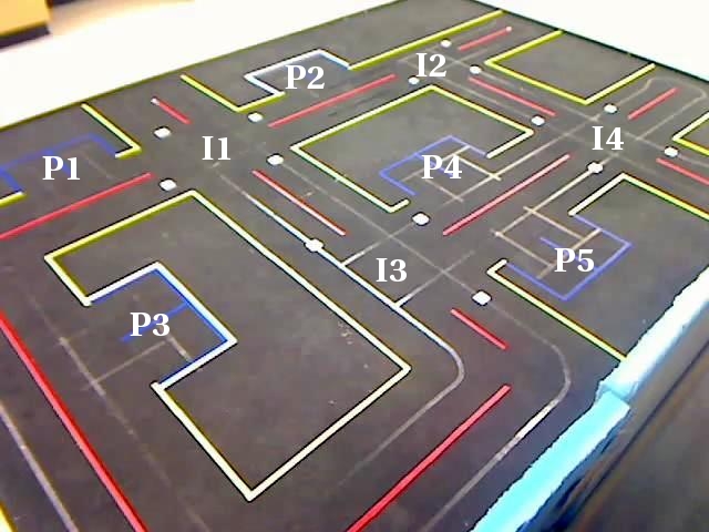
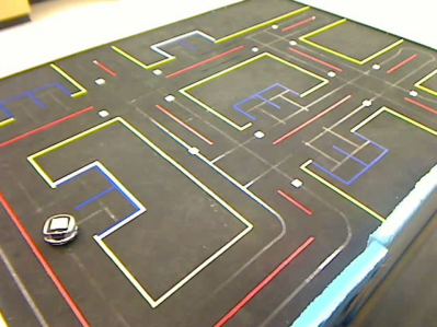
The goal of this paper is to plan the optimal motion of a robot subject to temporal logic constraints. This is an important problem in many applications where the robot has to perform a sequence of operations subject to external constraints. For example, in a persistent data gathering task the robot is tasked to gather data at several locations and then visit a different set of upload sites to transmit the data. Referring to Fig. 1, we would like to enable tasks such as “Repeatedly gather data at locations P1, P4, and P5. Upload data at either P2 or P3 after each data-gather. Follow the road rules, and avoid the road connecting I4 to I2.” We wish to determine robot motion that completes the task, and minimizes a cost function, such as the maximum time between data uploads.

Recently there has been an increased interest in using temporal logic to specify mission plans for robots [1, 2, 3, 4, 5, 6, 7]. Temporal logic is appealing because it provides a formal high level language in which to describe a complex mission. In addition, tools from model checking [8, 9, 10, 11] can be used to verify the existence of a robot trajectory satisfying the specification, and can produce a satisfying trajectory. However, frequently there are multiple robot trajectories that satisfy a given specification. In this case, one would like to choose the “optimal” trajectory according to a cost function. The current tools from model checking do not provide a method for doing this. In this paper we consider linear temporal logic specifications, and a particular form of cost function, and provide a method for computing optimal trajectories.

Figure 1: An environment consisting of roads, intersections and parking lots. An example mission in the environment is “Repeatedly gather data at locations P1, P4, and P5. Upload data at either P2 or P3 after each data-gather. Follow the road rules, and avoid the road connecting I4 to I2.”

The problem considered in this paper is related to the vehicle routing problem (VRP) [12]. The VRP is a generalization of the traveling salesman problem (TSP) in which the goal is to plan routes for vehicles to service customers. Vehicle routing extends the TSP by considering aspects such as multiple vehicles, vehicles with capacity constraints, and vehicles that must depart and return to specified depot locations. In [13], the authors consider a vehicle routing problem with metric temporal logic constraints. The goal is to minimize a cost function of the vehicle paths (such as total distance traveled). The authors present a method for computing an optimal solution by converting the problem to a mixed integer linear program (MILP). However, their method only applies to specifications where the temporal operators are applied only to atomic propositions. Thus, the method does not apply to persistent monitoring and data gathering problems, which have specifications of the form “always eventually.” In addition, the approach that we present in this paper leads to an optimization problem on a graph, rather than a MILP.

The contribution of this paper is to present a cost function for which we can determine an optimal robot trajectory that satisfies a general linear temporal logic formula. The cost function is motivated by problems in monitoring and data gathering, and it seeks to minimize the time between satisfying instances of a single optimizing proposition. Our solution, summarized in the Optimal-Run algorithm of Section IV, operates as follows. We represent the robot and environment as a weighted transition system. Then, we convert the linear temporal logic specification to a Büchi automaton. We synchronize the transition system with the Büchi automaton creating a product automaton. In this automaton a satisfying run is any run which visits a set of accepting state infinitely often. We show that there exists an optimal run that is in “prefix-suffix” structure, implying that we can search for runs with a finite transient, followed by a periodic steady-state. Thus, we create a polynomial time graph algorithm based on solutions of bottleneck shortest path problems to find an optimal cycle containing an accepting state. We implement our solution on the physical testbed shown in Fig. 1. We believe that optimizations of this type may be useful for a broader class of problems than the one considered here.

For simplicity of the presentation, we assume that the robot moves among the vertices of an environment modeled as a graph. However, by using feedback controllers for facet reachability and invariance in polytopes [14, 15, 16] the method developed in this paper can be easily applied for motion planning and control of a robot with “realistic” continuous dynamics (e.g., unicycle) traversing an environment partitioned using popular partitioning schemes such as triangulations and rectangular partitions.

The organization of the paper is as follows. In Section II we present preliminary results in temporal logic. In Section III we formally state the robot motion planning problem, and in Section IV we present our solution. In Section V we present results from a motion planning experiment for one robot in a road network environment. Finally in Section VI we present some promising future directions.

II Preliminaries

In this section we briefly review some aspects of linear temporal logic (LTL). LTL considers a finite set of variables $\Pi$, each of which can be either true or false. The variables $\alpha_{i}\in\Pi$ are called atomic propositions. In the context of robots, propositions can capture properties such as “the robot is located in region $1$”, or “the robot is recharging.”

Given a system model, LTL allows us to express the time evolution of the state of the system. We consider a type of finite model called the weighted transition system.

Definition II.1 (Weighted Transition System)

A weighted transition system is a tuple $\mathcal{T}:=(Q,q_{0},R,\Pi,\mathcal{L},w)$, consisting of (i) a finite set of states $Q$; (ii) an initial state $q_{0}\in Q$; (iii) a transition relation $R\subseteq Q\times Q$; (iv) a set of atomic propositions $\Pi$; (v) a labeling function $\mathcal{L}:Q\to 2^{\Pi}$; (vi) a weight function $w:R\to{\mathbb{R}}_{>0}$.

We assume that the transition system is non-blocking, implying that there is a transition from each state. The transition relation has the expected definition: given that the system is in state $q_{1}\in Q$ at time $t_{1}$, the system is in state $q_{2}$ at time $t_{1}+w\big{(}(q_{1},q_{2}))$ if and only if $(q_{1},q_{2})\in R$. The labeling function defines for each state $q\in Q$, the set $\mathcal{L}(q)$ of all atomic propositions valid in $q$. For example, the proposition “the robot is recharging” will be valid for all states $q\in Q$ containing recharging stations.

For our transition system we can define a run $r_{\mathcal{T}}$ to be an infinite sequence of states $q_{0}q_{1}q_{2}\ldots$ such that $q_{0}\in Q_{0}$, $q_{i}\in Q$, for all $i$, and $(q_{i},q_{i+1})\in R$, for all $i$. A run $r_{\mathcal{T}}$ defines a word $\mathcal{L}(q_{0})\mathcal{L}(q_{1})\mathcal{L}(q_{2})\ldots$ consisting of sets of atomic propositions valid at each state. An example of a weighted transition system is given in Fig. 2.

Figure 2: An example of a weighted transition system. A correct run of the system is for instance $q_{0}q_{2}q_{1}q_{0}q_{2}q_{3}q_{0}\ldots$, producing the word $\emptyset\{\text{gather}\}\{\text{upload}\}\emptyset\{\text{gather}\}\{\text{upload,recharge}\}\emptyset\ldots$.

Definition II.2 (Formula of LTL)

An LTL formula $\phi$ over the atomic propositions $\Pi$ is defined inductively as follows:

$$\phi::=\top\mid\alpha\mid\phi\lor\phi\mid\lnot\,\phi\mid\mathbf{X}\,\phi\mid\phi\,\mathcal{U}\,\phi$$

where $\top$ is a predicate true in each state of a system, $\alpha\in\Pi$ is an atomic proposition, $\neg$ (negation) and $\vee$ (disjunction) are standard Boolean connectives, and $\mathbf{X}$ and $\mathcal{U}$ are temporal operators.

LTL formulas are interpreted over infinite runs, as those generated by the transition system $\mathcal{T}$ from Def. II.1. Informally, $\mathbf{X}\,\alpha$ states that at the next state of a run, proposition $\alpha$ is true (i.e., $\alpha\in\mathcal{L}(q_{1})$). In contrast, $\alpha_{1}\,\mathcal{U}\,\alpha_{2}$ states that there is a future moment when proposition $\alpha_{2}$ is true, and proposition $\alpha_{1}$ is true at least until $\alpha_{2}$ is true. From these temporal operators we can construct two other useful operators Eventually (i.e., future), $\mathbf{F}$ defined as $\mathbf{F}\,\phi:=\top\,\mathcal{U}\,\phi$, and Always (i.e., globally), $\mathbf{G}$, defined as $\mathbf{G}\,\phi:=\lnot\,\mathbf{F}\,\lnot\,\phi$. The formula $\mathbf{G}\,\alpha$ states that proposition $\alpha$ holds at all states of the run, and $\mathbf{F}\,\alpha$ states that $\alpha$ holds at some future time instance.

An LTL formula can be represented in an automata-theoretic setting as Büchi automaton, defined as follows:

Definition II.3 (Büchi Automaton)

A Büchi automaton is a tuple $\mathcal{B}:=(S,S_{0},\Sigma,\delta,F)$, consisting of (i) a finite set of states $S$; (ii) a set of initial states $S_{0}\subseteq S$; (iii) an input alphabet $\Sigma$; (iv) a non-deterministic transition relation $\delta\subseteq S\times\Sigma\times S$; (v) a set of accepting (final) states $F\subseteq S$.

The semantics of Büchi automata are defined over infinite input words. Setting the input alphabet $\Sigma=2^{\Pi}$, the semantics are defined over the words consisting of sets of atomic propositions, i.e. those produced by a run of the transition system. Let $\omega=\omega_{0}\omega_{1}\omega_{2}\ldots$ be an infinite input word of automaton $\mathcal{B}$, where $\omega_{i}\in\Sigma$ for each $i\in\mathbb{N}$ (for example, the input $\omega=\mathcal{L}(q_{0})\mathcal{L}(q_{1})\mathcal{L}(q_{2})\ldots$ could be a word produced by a run $q_{0}q_{1}q_{2}\ldots$ of the transition system $\mathcal{T}$).

A run of the Büchi automaton over an input word $\omega=\omega_{0}\omega_{1}\omega_{2}\ldots$ is a sequence $r_{\mathcal{B}}=s_{0}s_{1}s_{2}\ldots$, such that $s_{0}\in S_{0}$, and $(s_{i},\omega_{i},s_{i+1})\in\delta$, for all $i\in\mathbb{N}$.

Definition II.4 (Büchi Acceptance)

A word $\omega$ is accepted by the Büchi automaton $\mathcal{B}$ if and only if there exists $r_{\mathcal{B}}$ over $\omega$ so that $\inf(r_{\mathcal{B}})\cap F\neq\emptyset$, where $\inf(r_{\mathcal{B}})$ denotes the set of states appearing infinitely often in run $r_{\mathcal{B}}$.

The Büchi automaton allows us to determine whether or not the word produced by a run of the transition system satisfies an LTL formula. More precisely, for any LTL formula $\phi$ over a set of atomic propositions $\Pi$, there exists a Büchi automaton $\mathcal{B}_{\phi}$ with input alphabet $2^{\Pi}$ accepting all and only the infinite words satisfying formula $\phi$ [8]. Translation algorithms were proposed in [17] and efficient implementations were developed in [18, 19]. The size of the obtained Büchi automaton is, in general, exponential with respect to the size of the formula. However, the exponential complexity is in practice not restrictive as the LTL formulas are typically quite small. An example of a Büchi automaton is given in Figure 3.

Figure 3: A Büchi automaton corresponding to LTL formula $(\mathbf{G}\,\mathbf{F}\,\mathrm{gather}\wedge\mathbf{G}\,\mathbf{F}\,\mathrm{upload})$ over the alphabet $\Pi$. The illustration of the automaton is simplified. In fact, each transition labeled with $\top$ represents $|2^{\Pi}|$ transitions labeled with all different subsets of atomic propositions. Similarly, a transition labeled with $\mathrm{gather}$ represent $|2^{\Pi}|/2$ transitions labeled with all subsets of atomic propositions containing the proposition $\mathrm{gather}$, etc.

III Problem Statement and Approach

Consider a single robot in an arbitrary environment, represented as a transition system (as defined in Section II) $\mathcal{T}=(Q,q_{0},R,\Pi,\mathcal{L},w)$. A run in the transition system starting at $q_{0}$ defines a corresponding trajectory of the robot in the environment. The time to take transition $(q_{1},q_{2})\in R$ (i.e., the time for the robot to travel from $q_{1}$ to $q_{2}$ in the environment) is given by $w(q_{1},q_{2})$.

To define our problem, we assume that there is an atomic proposition $\pi\in\Pi$, called the optimizing proposition. We consider LTL formulas of the form

$$\phi:=\varphi\land\mathbf{G}\,\mathbf{F}\,\pi.$$ (1)

The formula $\varphi$ can be any LTL formula over $\Pi$. The second part of the formula specifies that the proposition $\pi$ must be satisfied infinitely often, and will simply ensure well-posedness of our optimization.

Let each run of $\mathcal{T}$ start at time $t=0$, and assume that there is at least one run satisfying LTL formula (1). For each satisfying run $r_{\mathcal{T}}=q_{0}q_{1}q_{2}\ldots$, there is a corresponding word of sets of atomic propositions $\omega=\omega_{0}\omega_{1}\omega_{2}\ldots$, where $\omega_{i}=\mathcal{L}(q_{i})$. Associated with $r_{\mathcal{T}}$ there is a sequence of time instances $\mathbb{T}:=t_{0},t_{1},t_{2},\ldots$, where $t_{0}=0$, and $t_{i}$ denotes the time at which state $q_{i}$ is reached ($t_{i+1}=t_{i}+w(q_{i},q_{i+1})$). From this time sequence we can extract all time instances at which the proposition $\pi$ is satisfied. We let $\mathbb{T}_{\pi}$ denote the sequence of satisfying instances of the proposition $\pi$.

Our goal is to synthesize an infinite run $r_{\mathcal{T}}$ (i.e., a robot trajectory) satisfying LTL formula (1), and minimizing the cost function

$$\mathcal{C}(r_{\mathcal{T}})=\limsup_{i\to+\infty}\left(\mathbb{T}_{\pi}(i+1)-\mathbb{T}_{\pi}(i)\right),$$ (2)

where $\mathbb{T}_{\pi}(i)$ is the $i$th satisfying time instance of proposition $\pi$. Note that a finite cost in (2) enforces that $\mathbf{G}\,\mathbf{F}\,\pi$ is satisfied. Thus, the specification appears in $\phi$ merely to ensure that any satisfying run has finite cost. In summary, our goal is the following:

Problem Statement III.1

Determine an algorithm that takes as input a weighted transition system $\mathcal{T}$, an LTL formula $\phi$ in form (1), and an optimizing proposition $\pi$, and outputs a run $r_{\mathcal{T}}$ minimizing the cost $\mathcal{C}(r_{\mathcal{T}})$ in (2).

We now make a few remarks, motivating this problem.

Remarks III.2 (Comments on problem statement)

Cost function form: The transition system produces infinite runs. Thus, cost function (2) evaluates the steady-state time between satisfying instances of $\pi$. In the upcoming sections we design an algorithm that produces runs which reach steady-state in finite time. Thus, the runs produced will achieve the cost in (2) in finite time.

Expressivity of LTL formula (1): Many interesting LTL specifications can be cast in the form of (1). For example, suppose that we want to minimize the time between satisfying instances of a disjunction of propositions $\vee_{i}\alpha_{i}$. We can write this in the formula (1) by defining a new proposition $\pi$ which is satisfied at each state in which a $\alpha_{i}$ is satisfied.

In addition, the LTL formula $\varphi$ in (1) allows us to specify various rich robot motion requirements. An example of such is global absence ($\mathbf{G}\,\neg\psi$, globally keep avoiding $\psi$), response ($\mathbf{G}\,(\psi_{1}\Rightarrow\mathbf{F}\,\psi_{2})$, whenever $\psi_{1}$ holds true, $\psi_{2}$ will happen in future), reactivity ($\mathbf{G}\,\mathbf{F}\,\psi_{1}\Rightarrow\mathbf{G}\,\mathbf{F}\,\psi_{2}$, if $\psi_{1}$ holds in future for any time point, $\psi_{2}$ has to happen in future for any time point as well), sequencing ($\psi_{1}\,\mathcal{U}\,\psi_{2}\,\mathcal{U}\,\psi_{3}$, $\psi_{1}$ holds until $\psi_{2}$ happens, which holds until $\psi_{3}$ happens), and many others. For concrete examples, see Section V. $\square$

IV Problem Solution

In this section we describe our solution to Problem III.1. We leverage ideas from the automata-theoretic approach to model checking.

IV-A The Product Automaton

Consider the weighted transition system $\mathcal{T}=(Q,q_{0},R,\Pi,\mathcal{L},w)$, and a proposition $\pi\in\Pi$. In addition, consider an LTL formula $\phi=\varphi\land\mathbf{G}\,\mathbf{F}\,\pi$ over $\Pi$ in form (1), translated into a Büchi automaton $\mathcal{B}_{\phi}=(S,S_{0},2^{\Pi},\delta,F)$. With these two components, we define a new object, which we call the product automaton, that is suitably defined for our problem.

Definition IV.1 (Product Automaton)

The product automaton $\mathcal{P}=\mathcal{T}\times\mathcal{B}_{\phi}$ between the transition system $\mathcal{T}$ and the Büchi automaton $\mathcal{B}_{\phi}$ is defined as the tuple $\mathcal{P}:=(S_{\mathcal{P}},S_{\mathcal{P},0},\delta_{\mathcal{P}},F_{\mathcal{P}},w_{\mathcal{P}},S_{\mathcal{P},\pi})$, consisting of

1. a finite set of states $S_{\mathcal{P}}=Q\times S$,

2. a set of initial states $S_{\mathcal{P},0}=\{q_{0}\}\times S_{0}$,

3. a transition relation $\delta_{\mathcal{P}}\subseteq S_{\mathcal{P}}\times S_{\mathcal{P}}$, where $\big{(}(q,s),(\bar{q},\bar{s})\big{)}\in\delta_{\mathcal{P}}$ if and only if $(q,\bar{q})\in R$ and $(s,\mathcal{L}(q),\bar{s})\in\delta$.

4. a set of accepting (final) states $F_{\mathcal{P}}=Q\times F$.

5. a weight function $w_{\mathcal{P}}:\delta_{\mathcal{P}}\to{\mathbb{R}}_{>0}$, where $w_{\mathcal{P}}\big{(}(q,s),(\bar{q},\bar{s})\big{)}=w(q,\bar{q})$, for all $\big{(}(q,s),(\bar{q},\bar{s})\big{)}\in\delta_{\mathcal{P}}$.

6. a set of states $S_{\mathcal{P},\pi}\subseteq S_{\mathcal{P}}$ in which the proposition $\pi$ holds true. Thus, $(q,s)\in S_{\mathcal{P},\pi}$ if and only if $\pi\in\mathcal{L}(q)$.

The product automaton (as defined above) can be seen as a Büchi automaton with a trivial input alphabet. Since the alphabet is trivial, we omit it. Thus, we say that a run $r_{\mathcal{P}}$ in product automaton $\mathcal{P}$ is accepting if $\inf(r_{\mathcal{P}})\cap F_{\mathcal{P}}\neq\emptyset$. An example product automaton is illustrated in Fig. 4.

Figure 4: Product automaton between the transition system in Figure 2 and the Büchi automaton in Figure 3.

As in the transition system, we associate with each run $r_{\mathcal{P}}=p_{0}p_{1}p_{2}\ldots$, a sequence of time instances $\mathbb{T}_{\mathcal{P}}:=t_{0}t_{1}t_{2}\ldots$, where $t_{0}=0$, and $t_{i}$ denotes the time at which the $i$th vertex in the run is reached ($t_{i+1}=t_{i}+w_{\mathcal{P}}(p_{i},p_{i+1})$). From this time sequence we can extract a sequence $\mathbb{T}_{\mathcal{P},\pi}$, containing time instances $t_{i}$, where $p_{i}\in S_{\mathcal{P},\pi}$ (i.e. $\mathbb{T}_{\mathcal{P},\pi}$ is a sequence of satisfying instances of the optimizing proposition $\pi$ in $\mathcal{T}$). The cost of a run $r_{\mathcal{P}}$ on the product automaton $\mathcal{P}$ (which corresponds to cost function (2) on transition system $\mathcal{T}$) is

$$\mathcal{C}_{\mathcal{P}}(r_{\mathcal{P}})=\limsup_{i\to+\infty}\left(\mathbb{T}_{\mathcal{P},\pi}(i+1)-\mathbb{T}_{\mathcal{P},\pi}(i)\right).$$ (3)

The product automaton can also be viewed as a weighted graph, where the states define vertices of the graph and the transitions define the edges. Thus, we at times refer to runs of the product automaton as paths. A finite path is then a finite fragment of an infinite path.

Each accepting run of the product automaton can be projected to a run of the transition system satisfying the LTL formula. Formally, we have the following.

Proposition IV.2 (Product Run Projection, [8])

For any accepting run $r_{\mathcal{P}}=(q_{0},s_{0})(q_{1},s_{1})(q_{2},s_{2})\ldots$ of the product automaton $\mathcal{P}$, the sequence $r_{\mathcal{T}}=q_{0}q_{1}q_{2}\ldots$ is a run of $\mathcal{T}$ satisfying $\phi$. Furthermore, the values of cost functions $\mathcal{C}_{\mathcal{P}}$ and $\mathcal{C}$ are equal for runs $r_{\mathcal{P}}$ and $r_{\mathcal{T}}$, respectively.

Similarly, if $r_{\mathcal{T}}=q_{0}q_{1}q_{2}\ldots$ is a run of $\mathcal{T}$ satisfying $\phi$, then there exists an accepting run $r_{\mathcal{P}}=(q_{0},s_{0})(q_{1},s_{1})(q_{2},s_{2})\ldots$ of the product automaton $\mathcal{P}$, such that the values of cost functions $\mathcal{C}$ and $\mathcal{C}_{\mathcal{P}}$ are equal.

Finally, we need to discuss the structure of an accepting run of a product automaton $\mathcal{P}$.

Definition IV.3 (Prefix-Suffix Structure)

A prefix of an accepting run is a finite path from an initial state to an accepting state $f\in F_{\mathcal{P}}$ containing no other occurrence of $f$. A periodic suffix is an infinite run originating at the accepting state $f$ reached by the prefix, and periodically repeating a finite path originating and ending at $f$, and containing no other occurrence of $f$ (but possibly containing other vertices in $F_{\mathcal{P}}$). An accepting run is in prefix-suffix structure if it consists of a prefix followed by a periodic suffix.

Intuitively, the prefix can be thought of as the transient, while the suffix is the steady-state periodic behavior.

Lemma IV.4 (Prefix-Suffix Structure)

At least one of the accepting runs $r_{\mathcal{P}}$ of $\mathcal{P}$ that minimizes cost function $\mathcal{C}_{\mathcal{P}}(r_{\mathcal{P}})$ is in prefix-suffix structure.

Proof: Let $r_{\mathcal{P}}$ be an accepting run that minimizes cost function $\mathcal{C}_{\mathcal{P}}(r_{\mathcal{P}})$ and is not in prefix-suffix structure. We will prove the existence of an accepting run $\rho_{\mathcal{P}}$ in prefix-suffix structure, such that $\mathcal{C}_{\mathcal{P}}(\rho_{\mathcal{P}})\leq\mathcal{C}_{\mathcal{P}}(r_{\mathcal{P}})$. The idea behind the proof is that an accepting state must occur infinitely many times on $r_{\mathcal{P}}$. We then show that we can extract a finite path starting and ending at this accepting state which can be repeated to form a periodic suffix whose cost is no larger than $\mathcal{C}_{\mathcal{P}}(r_{\mathcal{P}})$.

To begin, there exists a state $f\in F_{\mathcal{P}}$ occurring on $r_{\mathcal{P}}$ infinitely many times. Run $r_{\mathcal{P}}$ consists of a prefix $r_{\mathcal{P}}^{\mathrm{fin}}$ ending at state $f$ followed by an infinite, non-periodic suffix $r_{\mathcal{P}}^{\mathrm{suf}}$ originating at the state $f$ reached by the prefix. The suffix $r_{\mathcal{P}}^{\mathrm{suf}}$ can be viewed as infinite number of finite paths of form $fp_{1}p_{2}\ldots p_{n}f$, where $p_{i}\neq f$ for any $i\in\{1,\ldots,n\}$. Let $\mathcal{R}$ denote the set of all finite paths of the mentioned form occurring on the suffix $r_{\mathcal{P}}^{\mathrm{suf}}$.

Note, that each path in the set $\mathcal{R}$ has to contain at least one occurrence of a state from $S_{\mathcal{P},\pi}$. To see this, assume by way of contradiction that there is a path $fp_{1}p_{2}\ldots p_{n}f$ that does not contain any state from $S_{P,\pi}$. The prefix $r_{\mathcal{P}}^{\mathrm{fin}}$ followed by infinitely many repetitions of this path is indeed an accepting run of $\mathcal{P}$. However, if projected into run of $\mathcal{T}$, formula $\mathbf{G}\,\mathbf{F}\,\pi$ and thus also formula $\phi$ is violated, contradicting Proposition IV.2.

Similarly as for infinite paths, we associate with each finite path of length $n$ a sequence of time instances $\mathbb{T}_{\mathcal{P}}:=t_{0}t_{1}t_{2}\ldots t_{n}$, where $t_{0}=0$, and $t_{i}$ denotes the time at which the $i$th vertex in the run is reached ($t_{i+1}=t_{i}+w_{\mathcal{P}}(p_{i},p_{i+1})$). From this time sequence we can extract a sequence $\mathbb{T}_{\mathcal{P},\pi}$, containing time instances $t_{i}$, where $p_{i}\in S_{\mathcal{P},\pi}$.

For each finite path $r\in\mathcal{R}$ with $n$ states and $k$ occurrences of a state from $S_{\mathcal{P},\pi}$ we define the following three costs

• $c^{f\leadsto}(r)=\mathbb{T}_{\mathcal{P},\pi}(0)-\mathbb{T}_{\mathcal{P}}(0)$

• $c(r)=\max_{i\in\{0,\ldots,k-1\}}\left(\mathbb{T}_{\mathcal{P},\pi}(i+1)-\mathbb{T}_{\mathcal{P},\pi}(i)\right)$

• $c^{\,\leadsto f}(r)=\mathbb{T}_{\mathcal{P}}(n)-\mathbb{T}_{\mathcal{P},\pi}(k)$.

Further, we define an equivalence relation $\sim$ over $\mathcal{R}$ as follows. Let $r_{1},r_{2}\in\mathcal{R}$. $r_{1}\sim r_{2}$ if and only if

• $c^{f\leadsto}(r_{1})=c^{f\leadsto}(r_{2})$,

• $c(r_{1})=c(r_{2})$, and

• $c^{\,\leadsto f}(r_{1})=c^{\,\leadsto f}(r_{2})$.

Costs $c^{f\leadsto}$, $c$, and $c^{\leadsto f}$ can be extended to $c^{f\leadsto}_{\sim}$, $c_{\sim}$, and $c^{\leadsto f}_{\sim}$ in a natural way. For example, we define $c^{f\leadsto}_{\sim}([r]_{\sim})=c^{f\leadsto}(r)$, where $r\in[r]_{\sim}$. The other two costs are defined analogously.

Let us extract a set $\mathcal{R}^{\mathrm{inf}}/_{\sim}$ from the set of equivalence classes $\mathcal{R}/_{\sim}$ such that each class in $\mathcal{R}^{\mathrm{inf}}/_{\sim}$ is infinite or contains a finite path that is repeated in $r_{\mathcal{P}}$ infinitely many times. As a consequence, for each class $[r]_{\sim}$ in $\mathcal{R}^{\mathrm{inf}}/_{\sim}$, it holds that $c_{\sim}([r]_{\sim})\leq\mathcal{C}_{\mathcal{P}}(r_{\mathcal{P}})$. The set $\mathcal{R}/_{\sim}$ is finite, because there is only a finite number of different values of costs. Furthermore, accepting run $r_{\mathcal{P}}$ is infinite and thus $\mathcal{R}^{\mathrm{inf}}/_{\sim}$ is nonempty.

Let $[\rho]_{\sim}\in\mathcal{R}^{\mathrm{inf}}/_{\sim}$ now be a class such that $c^{f\leadsto}_{\sim}([\rho]_{\sim})$ is minimal among the classes from $\mathcal{R}^{\mathrm{inf}}/_{\sim}$.

Each time a finite path in $[\rho]_{\sim}$ appears in $r_{\mathcal{P}}$, it is followed by another finite path. Consider, that infinitely many times the “following” path comes from a class $([r]_{\sim})\in\mathcal{R}^{\mathrm{inf}}/_{\sim}$. Then, we must have $c^{\leadsto f}([\rho]_{\sim})+c^{f\leadsto}([r]_{\sim})\leq\mathcal{C}_{\mathcal{P}}(r_{\mathcal{P}})$. But, $c^{f\leadsto}([r]_{\sim})\geq c^{\leadsto f}([\rho]_{\sim})$, and thus $c^{\leadsto f}([\rho]_{\sim})+c^{f\leadsto}([\rho]_{\sim})\leq\mathcal{C}_{\mathcal{P}}(r_{\mathcal{P}})$.

Thus we can build the run $\rho_{\mathcal{P}}$ as the prefix $r_{\mathcal{P}}^{\mathrm{fin}}$ followed by a periodic suffix $\rho_{\mathcal{P}}^{\mathrm{suf}}$, which is obtained by infinitely many repetitions of an arbitrary path $\rho\in[\rho]_{\sim}$. $\rho_{\mathcal{P}}$ is in prefix-suffix structure and for its suffix $\rho_{\mathcal{P}}^{\mathrm{suf}}$ it also holds $\mathcal{C}_{\mathcal{P}}(\rho_{\mathcal{P}})=\max_{i\in\mathbb{N}}\big{(}\mathbb{T}_{\mathcal{P},\pi}(i+1)-\mathbb{T}_{\mathcal{P},\pi}(i+1)\big{)}=\max\big{(}c(\rho),c^{f\leadsto}(\rho)+c^{\leadsto f}(\rho)\big{)}\leq\mathcal{C}_{\mathcal{P}}(r_{\mathcal{P}})$.   

Definition IV.5 (Suffix Cost)

The cost of the suffix $p_{0}p_{1}\ldots p_{n}p_{0}p_{1}\ldots$ of a run $r_{\mathcal{P}}$ is defined as follows. Let $t_{0,0},t_{0,1},\ldots,t_{0,n},t_{1,0},t_{1,1}\ldots$ be the sequence of times at which the vertices of the suffix are reached on run $r_{\mathcal{P}}$. Extract the sub-sequence $\mathbb{T}_{\mathcal{P}}^{\mathrm{suf}}$ of times $t_{i,j}$, where $p_{j}\in S_{\mathcal{P},\pi}$ (i.e. the satisfying instances of proposition $\pi$ in transition system $\mathcal{T}$). Then, the cost of the suffix is

$$\mathcal{C}_{\mathcal{P}}^{\mathrm{suf}}(r_{\mathcal{P}})=\max_{i\in\mathbb{N}}(\mathbb{T}_{\mathcal{P}}^{\mathrm{suf}}(i+1)-\mathbb{T}_{\mathcal{P}}^{\mathrm{suf}}(i)).$$

From the definition of the product automaton cost $\mathcal{C}_{\mathcal{P}}$ and the suffix cost $\mathcal{C}_{\mathcal{P}}^{\mathrm{suf}}$ we obtain the following result.

Lemma IV.6 (Cost of a Run)

Given a run $r_{\mathcal{P}}$ with prefix-suffix structure and its suffix $p_{0}p_{1}p_{2}\ldots p_{n}p_{0}p_{1}\ldots$, the value of the cost function $\mathcal{C}_{\mathcal{P}}(r_{\mathcal{P}})$ is equal to the cost of the suffix $\mathcal{C}_{\mathcal{P}}^{\mathrm{suf}}(r_{\mathcal{P}})$.

Our aim is to synthesize a run $r_{\mathcal{T}}$ of $\mathcal{T}$ minimizing the cost function $\mathcal{C}(r_{\mathcal{T}})$ and ensuring that the word produced by this run will be accepted by $\mathcal{B}$. This goal now translates to generating a run $r_{\mathcal{P}}$ of $\mathcal{P}$, such that the run satisfies the Büchi condition $F_{\mathcal{P}}$ and minimizes cost function $\mathcal{C}_{\mathcal{P}}(r_{\mathcal{P}})$. Furthermore, to find a satisfying run $r_{\mathcal{P}}$ that minimizes $\mathcal{C}_{\mathcal{P}}(r_{\mathcal{P}})$, it is enough to consider runs in prefix-suffix structure (see Lemma IV.4). From Lemma IV.6 it follows that the whole problem reduces to finding a periodic suffix $r_{\mathcal{P}}^{\mathrm{suf}}=fp_{1}p_{2}\ldots p_{n}fp_{1}\ldots$ in $\mathcal{P}$, such that:

1. $f$ is reachable from an initial state in $S_{\mathcal{P},0}$,

2. $f\in F_{\mathcal{P}}$ (i.e., $f$ is an accepting state), and

3. the cost of the suffix $r_{\mathcal{P}}^{\mathrm{suf}}$ is minimum among all the suffices satisfying (i) and (ii).

Finally, we can find a finite prefix in $\mathcal{P}$ leading from an initial state in $S_{\mathcal{P},0}$ to the state $f$ in the suffix $r_{\mathcal{P}}^{\mathrm{suf}}$. By concatenating the prefix and suffix, we obtain an optimal run in $\mathcal{P}$. By projecting the optimal run to $\mathcal{T}$, via Proposition IV.2, we obtain a solution to our stated problem.

IV-B Graph Algorithm for Shortest Bottleneck Cycles

We now focus on finding an optimal suffix in the product automaton. We cast this problem as path optimization on a graph. To do this, let us define some terminology.

A graph $G=(V,E,w)$ consists of a vertex set $V$, an edge set $E\subseteq V\times V$, and a weight function $w:E\to{\mathbb{R}}_{>0}$. A cycle in $G$ is a vertex sequence $v_{1}v_{2}\ldots v_{k}v_{k+1}$, such that $(v_{i},v_{i+1})\in E$ for each $i\in\{1,\ldots,k\}$, and $v_{1}=v_{k+1}$. Given a vertex set $S\subseteq V$, consider a cycle $c=v_{1}\ldots v_{k}v_{k+1}$ containing at least one vertex in $S$. Let $(i_{1},i_{2},\ldots,i_{s})$ be the ordered set of vertices in $c$ that are elements of $S$ (i.e., Indices with order $i_{1}<i_{2}<\cdots<i_{m}$, such that $v_{j}\in S$ if and only if $j\in\{i_{1},i_{2},\ldots,i_{s}\}$). Then, the $S$-bottleneck length is

$$\max_{\ell\in\{1,\ldots,s\}}\sum_{j=i_{\ell}}^{i_{\ell+1}-1}w(e_{j}),$$

where $i_{s+1}=i_{1}$. In words, we $S$-bottleneck distance is defined as follows.

Definition IV.7 ($S$-bottleneck length)

Given a graph $G=(V,E,w)$, and a vertex set $S\subseteq V$, the $S$-bottleneck length of a cycle in $G$ is the maximum distance between successive appearances of an element of $S$ on the cycle.

The bottleneck length of a cycle is defined as the maximum length edge on the cycle [20]. In contrast, the $S$-bottleneck length measures distances between vertices in $S$.

With the terminology in place, our goal is to solve the constrained $S$-bottleneck problem:

Problem Statement IV.8

Given a graph $G=(V,E,w)$, and two vertex sets $F,S\subseteq V$, find a cycle in $G$ containing at least one vertex in $F$, with minimum $S$-bottleneck length.

Our solution, shown in the Min-Bottleneck-Cycle algorithm, utilizes Dijkstra’s algorithm [20] for computing shortest paths between pairs of vertices (called Shortest-Path), and a slight variation of Dijkstra’s algorithm for computing shortest bottleneck paths between pairs of vertices (called Shortest-Bot-Path).

Shortest-Path takes as inputs a graph $G=(V,E,w)$, a set of source vertices $A\subseteq V$, and a set of destination vertices $B\subseteq V$. It outputs a distance matrix $D\in{\mathbb{R}}^{|A|\times|B|}$, where the entry $D(i,j)$ gives the shortest-path distance from $A_{i}$ to $B_{j}$. It also outputs a predecessor matrix $P\in V^{|A|\times|V|}$, where $P(i,j)$ is the predecessor of $j$ on a shortest path from $A_{i}$ to $V_{j}$. For a vertex $v\in V$, the shortest path from $v$ to $v$ is defined as the shortest cycle containing $v$. If there does not exist a path between vertices, then the distance is $+\infty$.

Shortest-Bot-Path has the same inputs as Shortest-Path, but it outputs paths which minimize the maximum edge length, rather than the sum of edge lengths.

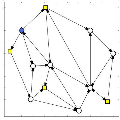
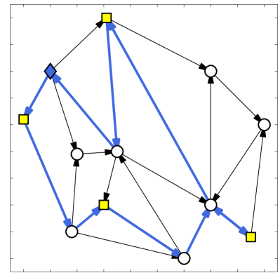
Fig. 5 (left) shows an example input to the algorithm. The graph contains 12 vertices, with one vertex (diamond) in $F$, and four vertices (square) in $S$. Fig. 5 (right) shows the optimal solution as produced by the algorithm. The bottleneck occurs between the square vertices immediately before and after the diamond vertex.

Input: : A directed graph $G$, and vertex subsets $F$ and $S$

Output: : A cycle in $G$ which contains at least one vertex in $F$ and minimizes the $S$-bottleneck distance.

1 Shortest paths between vertices in $S$:

$$(D,P)\leftarrow\textsc{Shortest-Path}(G,S,S).$$

;

2 Define a graph $G_{S}$ with vertices $S$ and adjacency matrix $D$. ;

3Shortest $S$-bottleneck paths between vertices in $S$:

$$(D_{\mathrm{bot}},P_{\mathrm{bot}})\leftarrow\textsc{Shortest-Bot-Path}(G_{S},S,S).$$

;

4 Shortest paths from each vertex in $F$ to each vertex in $S$, and from each vertex in $S$ to each vertex in $F$:

$$(D_{F\to S},P_{F\to S}) \leftarrow\textsc{Shortest-Path}(G,F,S)$$

$$(D_{S\to F},P_{S\to F}) \leftarrow\textsc{Shortest-Path}(G,S,F).$$

Set $D_{F\to S}(i,j)=0$ and $D_{S\to F}(j,i)=0$ for all $i,j$ such that $F_{i}=S_{j}$. ;

5For each triple $(f,s_{1},s_{2})\in F\times S\times S$, let $C(f,s_{1},s_{2})$ be $D_{F\to S}(f,s_{1})+D_{S\to F}(s_{2},f)$, if $f\neq s_{1}=s_{2}$, and $\max\big{\{}D_{F\to S}(f,s_{1})+D_{S\to F}(s_{2},f),D_{\mathrm{bot}}(s_{1},s_{2})\big{\}}$, otherwise.;

6Find the triple $(f^{*},s_{1}^{*},s_{2}^{*})$ that minimizes $C(f,s_{1},s_{2})$. ;

7If minimum cost is $+\infty$, then output “no cycle exists.” Else, output cycle by extracting the path from $f^{*}$ to $s_{1}^{*}$ using $P_{F\to S}$, the path from $s_{1}^{*}$ to $s_{2}^{*}$ using $P_{\mathrm{bot}}$ and $P$, and the path from $s_{2}^{*}$ to $f^{*}$ using $P_{S\to F}$. ;

Algorithm 1 Min-Bottleneck-Cycle$(G,S,F)$

Figure 5: A directed graph for illustrating the algorithm. The edge weights are given by the Euclidean distance. The set $F$ is a singleton given by the blue diamond. The vertices in $S$ are drawn as yellow squares. The thick blue edges in the right figure form a cycle with minimum $S$-bottleneck length.

In the algorithm, one has to take special care that cycle lengths are computed properly when $f=s_{1}$, $s_{1}=s_{2}$, or $f=s_{2}$. This is done by setting some entries of $D_{F\to S}$ and $D_{S\to F}$ to zero in step 4, and by defining the cost differently when $f\neq s_{1}=s_{2}$ in step 5. In the following theorem we show the correctness of the algorithm.

Theorem IV.9 (Min-Bottleneck-Cycle Optimality)

The Min-Bottleneck-Cycle algorithm solves the constrained $S$-bottleneck problem (Problem IV.8).

Proof: Every valid cycle must contain at least one element from $F$ and at least one element from $S$. Let $c:=v_{1}v_{2}\ldots v_{k}v_{1}$, be a valid cycle, and without loss of generality let $v_{1}\in F$. From this cycle we can extract the triple $(v_{1},v_{a},v_{b})\in F\times S\times S$, where$v_{a},v_{b}\in S$, and $v_{i}\notin S$ for all $i<a$ and for all $i>b$. (Note that, $a=b=1$ is possible.)

Consider a cycle $c$ with corresponding triple $(f,s_{1},s_{2})$, and let $L(c)$ denote its $S$-bottleneck length. It is straightforward to verify, using the definition of $S$-bottleneck length, that $L(c)\geq C(f,s_{1},s_{2})$.

The cycle computed in step 5 (as given by the four predecessor matrices) takes the shortest path from $f$ to $s_{1}$, the shortest $S$-bottleneck path from $s_{1}$ to $s_{2}$, and the shortest path from $s_{2}$ to $f$. However, the shortest path from $f$ to $s_{1}$ (and from $s_{2}$ to $f$) may contain other vertices from $S$. Thus, the $S$-bottleneck length of this cycle, denoted $L(f,s_{1},s_{2})$, satisfies

$$L(f,s_{1},s_{2})\leq C(f,s_{1},s_{2})\leq L(c),$$ (4)

implying that $C(f,s_{1},s_{2})$ upper bounds the length of the computed cycle. However, if we take $c$ to be a cycle with minimum length, then necessarily $L(c)\leq L(f,s_{1},s_{2})$. Hence, equation (4) implies that for an optimal cycle, $L(f,s_{1},s_{2})=C(f,s_{1},s_{2})=L(c)$. Thus, by minimizing the cost function in step 5 we compute the minimum length cycle.   

Computational Complexity: Finally, we characterize the computational complexity of the Min-Bottleneck-Cycle algorithm. Let $n$, $m$, $n_{S}$, and $n_{F}$, be the number of vertices (edges) in the sets $V$, $E$, $S$, and $F$, respectively. Dijkstra’s algorithm can be implemented to compute shortest paths from a source vertex $v\in V$, to all other vertices in $V$ in $O(n\log n+m)$ run time. Thus, for sparse graphs (which includes many transition systems), the run time is $O(n\log n)$.

Proposition IV.10 (Min-Bottleneck-Cycle run time)

The run time of the Min-Bottleneck-Cycle algorithm is $O\big{(}(n_{S}+n_{F})(n\log n+m+n_{S}^{2})\big{)}$. Thus, in the worst-case, the run time is $O(n^{3})$. For sparse graphs with $n_{S},n_{F}\ll n$, the run time is $O\big{(}(n_{S}+n_{F})n\log n\big{)}$.

Proof: We simply look at the run time of each step in the algorithm. Step 1 requires $n_{S}$ calls to Dijkstra’s algorithm, and has run time $O(n_{S}(n\log(n)+m))$. Step 3 requires $n_{S}$ calls to Dijkstra’s algorithm on a smaller graph $G_{S}=(S,E_{S},w_{S})$, and has run time $O(n_{S}(n_{S}\log(n_{S})+|E_{S}|))$. Step 4 has run time $O(n_{F}(n\log(n)+m))$. Finally, step 5 and 6 require searching over all $n_{F}\cdot n_{S}^{2}$ possibilities, and have run time $O(n_{F}n_{S}^{2})$. Since $|E_{S}|\leq n_{S}^{2}$, the run time in general is given by $O\big{(}(n_{S}+n_{F})(n\log n+m+n_{S}^{2})\big{)}$.   

IV-C The Optimal-Run algorithm

We are now ready to combine the results from the previous section to present a solution to Problem III.1. The solution is summarized in the Optimal-Run algorithm.

Input: : A weighted transition system $\mathcal{T}$, and temporal logic specification $\phi$ in form (1).

Output: : A run in $\mathcal{T}$ which satisfies $\phi$ and minimizes (2).

1Convert $\phi$ to a Büchi automaton $\mathcal{B}_{\phi}$. ;

2Compute the product automaton $\mathcal{P}=\mathcal{T}\times\mathcal{B}_{\phi}$. ;

3 Compute the cycle Min-Bottleneck-Cycle$(G,S_{\mathcal{P},\pi},F_{\mathcal{P}})$, where $G=(S_{\mathcal{P}},\delta_{\mathcal{P}},w_{\mathcal{P}})$. ;

4 Compute a shortest path from $S_{\mathcal{P},0}$ to the cycle. ;

5Project the complete run (path and cycle) to a run on $\mathcal{T}$ using Proposition IV.2. ;

Algorithm 2 Optimal-Run$(\mathcal{T},\phi)$

Combining Lemma IV.4, Theorem IV.9, and Proposition IV.2, we obtain the following result.

Theorem IV.11 (Correctness of Optimal-Run)

The Optimal-Run algorithm solves Problem III.1.

V Experiments

We have implemented the Optimal-Run algorithm in simulation and on a physical road network testbed. The road network shown in Fig. 1 is a collection of roads, intersections, and parking lots, connected by a simple set of rules (e.g., a road connects two (not necessarily different) intersections, the parking lots can only be located on the side of a road). The city is easily reconfigurable through re-taping. The robot is a Khepera III miniature car. The car can sense when entering an intersection from a road, when entering a road from an intersection, when passing in front of a parking lot, when it is correctly parked in a parking space, and when an obstacle is dangerously close. The car is programmed with motion and communication primitives allowing it to safely drive on a road, turn in an intersection, and park. The car can communicate through Wi-Fi with a desktop computer, which is used as an interface to the user (i.e., to enter the specification) and to perform all the computation necessary to generate the control strategy. Once computed, this is sent to the car, which executes the task autonomously by interacting with the environment.

Modeling the motion of the car in the road network using a weighted transition system (Def. II.1) is depicted in Fig. 6 and proceeds as follows. The set of states $Q$ is the set of labels assigned to the intersections, parking lots, and branching points between the roads and parking lots. The transition relation $R$ shows how the regions are connected and the transitions’ labels give distances between them (measured in inches). In our testbed the robot moves at constant speed $\nu$, and thus the distances and travel times are equivalent. For these experiments, the robot can only move on right hand lane of a road and it cannot make a U-turn at an intersection. To capture this, we model each intersection as four different states. Note that, in reality, each state in $Q$ has associated a set of motion primitives, and the selection of a motion primitive (e.g., go_straight, turn_right) determines the transition to one unique next states. This motivates our assumption that the weighted transition system from Def. II.1 is deterministic, and therefore its inputs can be removed.

\begin{picture}(6864.0,4501.0)(1761.0,-8886.0)\end{picture}

Figure 6: The weighted transition system for the road network in Fig. 1.

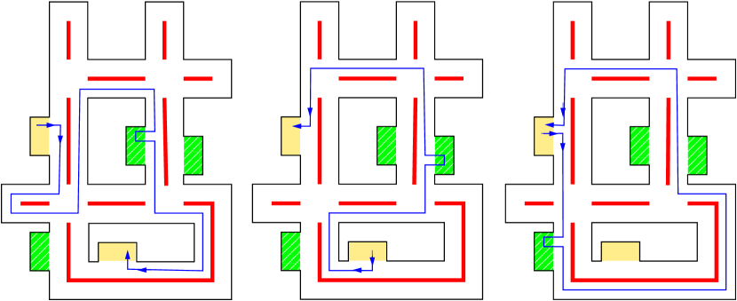
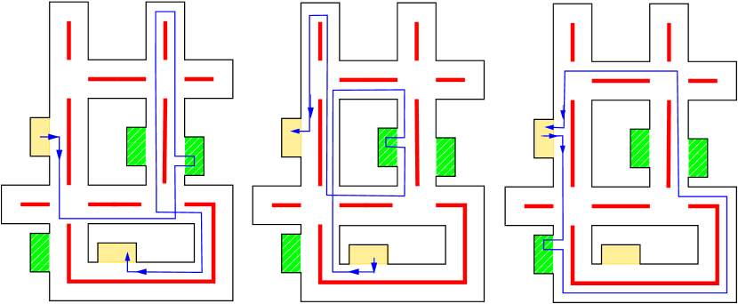
In our experiment, we have considered the following task. Parking spots $\mathrm{P2}$ and $\mathrm{P3}$ in Fig. 6 are data upload locations (light shaded in Fig. 8) and parking spots $\mathrm{P1}$, $\mathrm{P4}$, and $\mathrm{P5}$ are data gather locations (dark shaded in Fig. 8). The optimizing proposition $\pi$ in LTL formula (1) is $\pi:=\mathrm{P2}\vee\mathrm{P3}$, i.e. we want to minimize the time between data uploads. Both upload locations provide the same service. On the other hand, data gather locations are unique and provide the robot with different kind of data. Assuming infinite runs of the robot in the environment, the motion requirements can be specified as LTL formulas, where atomic propositions are simply names of the parking spots. Namely, in the formula $\varphi$ of the LTL formula (1), we demand the conjunction of the following:

• The robot keeps visiting each data gather location.

  $$\mathbf{G}\,\mathbf{F}\,\mathrm{P1}\wedge\mathbf{G}\,\mathbf{F}\,\mathrm{P4}\wedge\mathbf{G}\,\mathbf{F}\,\mathrm{P5}$$

• Whenever the robot gathers data, it uploads it before doing another data gather.

  $$\mathbf{G}\,((\mathrm{P1}\vee\mathrm{P4}\vee\mathrm{P5})\Rightarrow\mathbf{X}\,(\neg(\mathrm{P1}\vee\mathrm{P4}\vee\mathrm{P5})\,\mathcal{U}\,(\mathrm{P2}\vee\mathrm{P3})))$$

• Whenever the robot uploads data, it does not visit an upload location again before gathering new data.

  $$\mathbf{G}\,((\mathrm{P2}\vee\mathrm{P3})\Rightarrow\mathbf{X}\,(\neg(\mathrm{P2}\vee\mathrm{P3})\,\mathcal{U}\,(\mathrm{P1}\vee\mathrm{P4}\vee\mathrm{P5})))$$

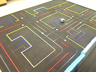
Note that the above specifications implicitly enforce $\mathbf{G}\;\mathbf{F}\;\pi$. Running the Optimal-Run algorithm, we obtain the solution as illustrated in the top three environment shots in Fig. 8. The transition system has 26 states, and the Büchi automaton had 16 states, giving a product automaton with 416 states. In the product automaton, $F_{\mathcal{P}}$ contained 52 states, and $S_{\mathcal{P},\pi}$ contained 32 states. The Optimal-Run algorithm ran in approximately 6 seconds on a standard laptop. The value of the cost function was 9.13 meters, which corresponded to a robot travel time of 3.6 minutes (i.e., the maximum travel time between uploads was 3.6 minutes). Our video submission displays the robot trajectory for this run and Fig. 7 shows two snapshots from the video.

Figure 7: Two snapshots of the robot in road network. In the left figure the robot is gathering data, and in the right figure it is about to upload.

The bottom three shots in Fig. 8 illustrate the situation with the same motion requirements and a further restriction saying that the robot cannot upload data in $\mathrm{P2}$ after data is gathered in location $\mathrm{P5}$: $\mathbf{G}\,(\mathrm{P5}\Rightarrow(\neg\mathrm{P2}\,\mathcal{U}\,\mathrm{P3}))$. In this case the Büchi automaton contained 29 states, the algorithm ran in 22 seconds, and the value of the cost function was 9.50 meters with a travel time of 3.77 minutes.

Figure 8: The robot trajectories (blue arrows) for the data gathering mission. Green (dark shaded) areas are data-gathering locations, and yellow (light shaded) areas are upload locations. The bottom three figures show the new robot trajectory when we restrict data upload to location $\mathrm{P3}$ (the bottom yellow location) after each data-gather at $\mathrm{P5}$ (the rightmost green location).

VI Conclusions and Future Directions

In this paper we presented a method for planning the optimal motion of a robot subject to temporal logic constraints. The problem is important in applications where the robot has to perform a sequence of operations subject to external constraints. We considered temporal logic specifications which contain a single optimizing proposition that must be repeatedly visited. We provided a method for computing a valid robot trajectory that minimizes the maximum time between satisfying instances of the optimizing proposition. We demonstrated our method for a robotic data gathering mission in a city environment.

There are many promising directions for future work. We are looking at ways to extend the cost functions that can be optimized. In particular, we are looking at extensions to more general types of patrolling problems. Another interesting direction is the extension to multiple robots. This naturally leads to developing solutions that are distributed among the robots.

References

- [1] M. Antoniotti and B. Mishra, “Discrete event models + temporal logic = supervisory controller: Automatic synthesis of locomotion controllers,” in IEEE Int. Conf. on Robotics and Automation, Nagoya, Japan, 1995, pp. 1441–1446.
- [2] S. G. Loizou and K. J. Kyriakopoulos, “Automatic synthesis of multiagent motion tasks based on LTL specifications,” in IEEE Conf. on Decision and Control, Paradise Island, Bahamas, 2004, pp. 153–158.
- [3] M. M. Quottrup, T. Bak, and R. Izadi-Zamanabadi, “Multi-robot motion planning: A timed automata approach,” in IEEE Int. Conf. on Robotics and Automation, New Orleans, LA, 2004, pp. 4417–4422.
- [4] C. Belta, V. Isler, and G. J. Pappas, “Discrete abstractions for robot motion planning and control in polygonal environment,” IEEE Transactions on Robotics, vol. 21, no. 5, pp. 864–875, 2005.
- [5] G. E. Fainekos, H. Kress-Gazit, and G. J. Pappas, “Temporal logic motion planning for mobile robots,” in IEEE Int. Conf. on Robotics and Automation, Barcelona, Spain, Apr. 2005, pp. 2032–2037.
- [6] H. Kress-Gazit, G. Fainekos, and G. J. Pappas, “Where’s Waldo? Sensor-based temporal logic motion planning,” in IEEE Int. Conf. on Robotics and Automation, Rome, Italy, 2007, pp. 3116–3121.
- [7] T. Wongpiromsarn, U. Topcu, and R. M. Murray, “Receding horizon temporal logic planning for dynamical systems,” in IEEE Conf. on Decision and Control, Shanghai, China, 2009, pp. 5997–6004.
- [8] M. Y. Vardi and P. Wolper, “An automata-theoretic approach to automatic program verification,” in Logic in Computer Science, 1986, pp. 322–331.
- [9] G. Holzmann, “The model checker SPIN,” IEEE Transactions on Software Engineering, vol. 25, no. 5, pp. 279–295, 1997.
- [10] E. M. Clarke, D. Peled, and O. Grumberg, Model checking. MIT Press, 1999.
- [11] J. Barnat, L. Brim, and P. Ročkai, “DiVinE 2.0: High-performance model checking,” in High Performance Computational Systems Biology. IEEE Computer Society Press, 2009, pp. 31–32.
- [12] P. Toth and D. Vigo, Eds., The Vehicle Routing Problem, ser. Monographs on Discrete Mathematics and Applications. SIAM, 2001.
- [13] S. Karaman and E. Frazzoli, “Vehicle routing problem with metric temporal logic specifications,” in IEEE Conf. on Decision and Control, Cancún, México, 2008, pp. 3953–3958.
- [14] L. C. G. J. M. Habets and J. H. van Schuppen, “A control problem for affine dynamical systems on a full-dimensional polytope,” Automatica, vol. 40, pp. 21–35, 2004.
- [15] L. Habets, P. Collins, and J. van Schuppen, “Reachability and control synthesis for piecewise-affine hybrid systems on simplices,” IEEE Transactions on Automatic Control, vol. 51, pp. 938–948, 2006.
- [16] C. Belta and L. Habets, “Control of a class of nonlinear systems on rectangles,” IEEE Transactions on Automatic Control, vol. 51, no. 11, pp. 1749–1759, 2006.
- [17] M. Y. Vardi and P. Wolper, “Reasoning about infinite computations,” Information and Computation, vol. 115, pp. 1–37, 1994.
- [18] R. Gerth, D. Peled, M. Vardi, and P. Wolper, “Simple on-the-fly automatic verification of linear temporal logic,” in Protocol Specification, Testing and Verification. Chapman & Hall, 1995, pp. 3–18.
- [19] P. Gastin and D. Oddoux, “Fast LTL to Büchi automata translation,” in Conf. on Computer Aided Verification, ser. Lecture Notes in Computer Science, no. 2102. Springer, 2001, pp. 53–65.
- [20] B. Korte and J. Vygen, Combinatorial Optimization: Theory and Algorithms, 4th ed., ser. Algorithmics and Combinatorics. Springer, 2007, vol. 21.