Measuring Unification

Abstract

If supersymmetry is observed at the LHC its model parameters can be measured at the electroweak scale. We discuss the expected precision on the parameter determination, including a proper treatment of experimental and theoretical errors. Particular attention is paid to degenerate solutions. Using the SFitter framework we perform a bottom-up reconstruction of the unified parameters at the high scale, including a full error propagation.

1 Introduction

While supersymmetry was originally not introduced as a phenomenological model targeted at definite shortcomings of our Standard Model, it has since developed into the most attractive ultraviolet completion of the Standard Model at and above the TeV scale. The basis of supersymmetric theories is a matching of fermionic degree of freedom with bosonic degree of freedom, now given the particle content of the Standard Model at the electroweak scale Nath:2010zj ; review ; Martin:1997ns . This symmetry automatically cures the theoretical problem with a perturbatively unstable fundamental Higgs mass in the Standard Model, i.e. the hierarchy problem.

Several specific points make the minimal supersymmetric extension of the Standard Model (MSSM) an attractive ultraviolet completion: while electroweak precision data favors a light Higgs boson Alcaraz:2007ri , supersymmetry provides such a lightest Higgs boson with a mass less than about 140 GeV. To implement fundamental symmetries protecting the proton life time and avoiding flavor-changing neutral currents into the MSSM we usually resort to $R$ parity. This parity in turn forces the lightest supersymmetric particle to be stable. Attributed to a ‘WIMP miracle’ the typical relic densities predicted for a weakly interacting supersymmetric dark matter candidate roughly agree with the observed values dm_review1 ; dm_review2 .

In addition to these attractive weak-scale properties supersymmetry offers another, unique, opportunity: it allows us to predictively extrapolate a perturbative and renormalizable gauge theory to arbitrarily high energy scales. While we know that the three gauge couplings do not unify in the Standard Model, including supersymmetric degrees of freedom at the TeV scale can naturally lead to such a unification angle1 ; angle2 ; angle3 ; angle4 ; angle5 ; Marciano:1981un ; angle6 . This is one of the reasons why fundamental and unbroken supersymmetry could live above the unification scale $Q_{\text{GUT}}>10^{16}$ GeV msugra1 ; msugra2 ; msugra3 ; msugra4 ; msugra5 ; msugra6 ; msugra7 ; msugra8 ; msugra9 . One way of breaking supersymmetry would then be a gravity-driven link between a hidden sector and the MSSM, where the scales get adjusted to accommodate supersymmetry-breaking mass parameters around the TeV scale. Using this setup a renormalization group analysis shows that the electroweak symmetry is automatically broken by running one of the two Higgs masses squared to negative values slightly below the mass scale of the supersymmetric partners Nilles:1982ik .

In the coming years supersymmetry should be discovered at the LHC. An e⁺e^- linear collider (ILC) with a center–of–mass energy of 500 GeV extendible to 1 TeV, as it is under study, can shed further light on supersymmetry. A formidable task will be to determine the fundamental parameters of supersymmetry from experimental measurements. Even if we expect supersymmetry to unify at a high scale we should not assume such a unification and simply fit the high-scale parameters to experimental measurements at the electroweak scale. Instead, the appropriate though technically challenging question should be: do the measured weak-scale MSSM parameters evolved to high energy scales unify? Or, if not, can we observe relics of a unification, like sum rules stable with respect to renormalization group running sumrules .

In principle, grand unification of the supersymmetric parameters can be observed from data in the gaugino and scalar sectors Blair:2002pg ; Allanach:2004ud ; Kneur:2008ur or in the gaugino sector only Altunkaynak:2009tg . The aspect we focus on in this study is the determination of the central values and errors Lafaye:2004cn ; Lafaye:2007vs , i.e. a proper measurement of supersymmetric unification. The bottom-up renormalization group analysis are performed for expected LHC measurements and its combination with the ILC. Because our analysis depends critically on the knowledge of all errors, we use the well studied parameter set SPS1a Allanach:2002nj . It is interesting to note that the result of the fit of the electroweak data, adding b–physics observables, the anomalous magnetic moment of the muon Davier:2009zi and the relic density Larson:2010gs , yields a best–fit point not too far from SPS1a, a further motivation to study in detail such a parameter choice Buchmueller:2007zk ; Bechtle:2009ty ; Buchmueller:2008qe . Note that by adjusting slightly the parameters of SPS1a (denoted SPS1a’ or SPA1 in AguilarSaavedra:2005pw ) the relic density can be reduced to agree with the measurement from WMAP Larson:2010gs without changing the collider observables significantly. The relic density is only a side product of our analysis, therefore we stick to SPS1a for which the experimental error estimates are available directly.

Our analysis relies on the SFitter framework Lafaye:2004cn ; Lafaye:2007vs . The same techniques have been successfully applied to other questions, like the determination of the Higgs boson couplings at the LHC Lafaye:2009vr . The theoretical aspects of evolving the relevant parameters from the electroweak to the GUT scale and vice-versa we discussed in Section 2. The expected measurements at the LHC and ILC are listed in Section 3, followed by a summary of the determination of the MSSM parameters at the electroweak scale in Section 4. In Section 5 we develop the method for the determination of the unified parameters at the high scale and apply it to the respective LHC and LHC+ILC measurements.

2 Theoretical aspects

For the following studies, the MSSM is defined as a variant of the phenomenological MSSM with the following parameters (evaluated for convenience at the electroweak scale, 1 TeV AguilarSaavedra:2005pw ): $\tan\beta$ is the ratio of the vacuum expectation values of the Higgs doublets, $\mathrm{M}_{1}$, $\mathrm{M}_{2}$ and $\mathrm{M}_{3}$ are the gaugino mass parameters, $\mu$ is the higgsino supersymmetric mass parameter and $m_{A}$ the physical (pole) mass of the pseudo scalar Higgs boson. For simplicity the gaugino masses are restricted to be positive. The soft breaking masses in the slepton sector are denoted as $\mathrm{M}_{\tilde{\mathrm{e}}_{\mathrm{L}}}$, $\mathrm{M}_{\tilde{\mathrm{e}}_{\mathrm{R}}}$, $\mathrm{M}_{\tilde{\mu}_{\mathrm{L}}}$, $\mathrm{M}_{\tilde{\mu}_{\mathrm{R}}}$, $\mathrm{M}_{\tilde{\tau}_{\mathrm{L}}}$ and $\mathrm{M}_{\tilde{\tau}_{\mathrm{R}}}$. For the squarks, as u, d, s and c quarks are experimentally practically indistinguishable, a common definition (average) is used for the first two generations denoted as $\mathrm{M}_{\tilde{\mathrm{q}}_{\mathrm{L}}}$ and $\mathrm{M}_{\tilde{\mathrm{q}}_{\mathrm{R}}}$. The third generation is treated separately with the parameters $\mathrm{M}_{{\tilde{\mathrm{q}}3}_{\mathrm{L}}}$, $\mathrm{M}_{\tilde{\mathrm{t}}_{\mathrm{R}}}$ and $\mathrm{M}_{\tilde{\mathrm{b}}_{\mathrm{R}}}$. The tri-linear terms, irrelevant for the first two generations due to the smallness of the fermion masses, are taken into account for the third generation with $\mathrm{A}_{\tau}$, $\mathrm{A}_{t}$ and $\mathrm{A}_{b}$.

The supersymmetric and soft-supersymmetry breaking parameters of the MSSM can in principle be defined at some arbitrary scale, not only the electroweak scale. In order to compare the results of the bottom-up and top-down approach, the high scale MSSM will also be used. The parameters of this model are defined at the GUT scale ($\sim 10^{16}$ GeV). In this model the two weak scale parameters $\mu$ and $m_{A}$ are replaced with the soft supersymmetry-breaking terms for the Higgs doublets, $\mathrm{M}_{\mathrm{H}_{1}}$ and $\mathrm{M}_{\mathrm{H}_{2}}$.

2.1 Renormalization Group Evolution properties

type of		nominal	stat.	LES	JES	theo.
measurement		value	error
$m_{h}$		108.7	0.01	0.25		2.0
$m_{t}$		171.20	0.01		1.0
$m_{\tilde{l}_{L}}-m_{\chi_{1}^{0}}$		102.38	2.3	0.1		1.1
$m_{\tilde{g}}-m_{\chi_{1}^{0}}$		511.38	2.3		6.0	6.1
$m_{\tilde{q}_{R}}-m_{\chi_{1}^{0}}$		446.39	10.0		4.3	5.5
$m_{\tilde{g}}-m_{\tilde{b}_{1}}$		89.01	1.5		1.0	8.0
$m_{\tilde{g}}-m_{\tilde{b}_{2}}$		62.93	2.5		0.7	8.2
$m_{ll}^{\mathrm{max}}$:	three-particle edge($\chi_{2}^{0}$,$\tilde{l}_{R}$,$\chi_{1}^{0}$)	80.852	0.042	0.08		1.2
$m_{llq}^{\mathrm{max}}$:	three-particle edge($\tilde{q}_{L}$,$\chi_{2}^{0}$,$\chi_{1}^{0}$)	449.08	1.4		4.3	5.1
$m_{lq}^{\mathrm{low}}$:	three-particle edge($\tilde{q}_{L}$,$\chi_{2}^{0}$,$\tilde{l}_{R}$)	326.32	1.3		3.0	5.2
$m_{ll}^{\mathrm{max}}(\chi_{4}^{0})$:	three-particle edge($\chi_{4}^{0}$,$\tilde{l}_{L}$,$\chi_{1}^{0}$)	277.36	3.3	0.3		2.0
$m_{\tau\tau}^{\mathrm{max}}$:	three-particle edge($\chi_{2}^{0}$,$\tilde{\tau}_{1}$,$\chi_{1}^{0}$)	83.21	5.0		0.8	1.0
$m_{lq}^{\mathrm{high}}$:	four-particle edge($\tilde{q}_{L}$,$\chi_{2}^{0}$,$\tilde{l}_{R}$,$\chi_{1}^{0}$)	390.18	1.4		3.8	5.0
$m_{llq}^{\mathrm{thres}}$:	threshold($\tilde{q}_{L}$,$\chi_{2}^{0}$,$\tilde{l}_{R}$,$\chi_{1}^{0}$)	216.00	2.3		2.0	3.3
$m_{llb}^{\mathrm{thres}}$:	threshold($\tilde{b}_{1}$,$\chi_{2}^{0}$,$\tilde{l}_{R}$,$\chi_{1}^{0}$)	198.41	5.1		1.8	3.1

Table 1: LHC measurements in SPS1a, taken from Weiglein:2004hn . Shown are the nominal values (from SUSPECT Djouadi:2002ze ) and statistical errors, systematic errors from the lepton (LES) and jet energy scale (JES) and theoretical errors. All values are given in GeV.

The renormalization group equations (RGE) RGE2 play an important role in the analysis by relating low to high scale MSSM parameters. Corrections up to the level of two–loops are implemented in SUSPECT Djouadi:2002ze and SoftSUSY Allanach:2001kg . Three-loop results for the beta functions are known and have been shown to stay within the two-loop error bands 3loop1 ; 3loop2 . Unless stated otherwise the full two-loop corrections are applied in the following. An approximate analytical form is useful to understand the RGE dependence of the most relevant parameters. Typically, at leading one-loop order the RGE for the gaugino mass parameters are closely related to the ones for the gauge coupling RGE2 :

$$\frac{d}{dt}(\ln\mathrm{M}_{i}(t))=\frac{B_{i}}{8\pi^{2}}g^{2}_{i}=\frac{d}{dt}(\ln g^{2}_{i})\;,$$ (1)

where $t=\ln Q$, $B_{i}=(33/5,1,-3)$ and $\mathrm{M}_{i}$, $g_{i}$ for $i=1,2,3$ are the gaugino masses and gauge couplings (in the standard normalization with $g_{1}=\sqrt{5/3}\,g_{Y}$). This immediately implies

$$\frac{\mathrm{M}_{i}(Q)}{g^{2}_{i}(Q)}=\mbox{constant}\equiv\frac{\mathrm{M}_{i}(Q_{in})}{g^{2}_{i}(Q_{in})}$$ (2)

where $Q_{in}$ is an arbitrary initial scale, either the high scale for top-down or the low scale for bottom-up evolution. More explicitly, the one-loop RGE solutions for the gauge couplings lead to

$$\mathrm{Z}_{i} = \left[1+\frac{B_{i}}{4\pi}\alpha_{i}(Q_{in})\,\ln(\mathrm{Q}^{2}/\mathrm{Q_{in}}^{2})\right]^{-1}$$

$$\mathrm{M}_{i}(Q) = \mathrm{Z}_{i}\mathrm{M}_{i}(Q_{in})$$ (3)

where $\alpha_{i}\equiv g^{2}_{i}/(4\pi)$.

The structure of the RGE thus shows that the gaugino sector is essentially determined by gauge couplings, and to some extent by the Yukawa couplings which only enter at the two-loop level. The gaugino parameters are decoupled from the scalar sector. In contrast, the soft parameters in the scalar sector are strongly correlated due to the RGE: most of the soft scalar masses depend not only on their value at the initial scale, but also on other scalar masses as well as gaugino mass and trilinear coupling parameters. An approximation of those solutions for all possible scalar masses can be written e.g. in terms of high scale universal $m_{0},m_{1/2},A_{0}$ parameters, but these are not very useful and can even be misleading. The RGE for the slepton and squark parameters of the first two generations, $\mathrm{M}_{\tilde{\mathrm{e}}_{\mathrm{R}}}$, $\mathrm{M}_{\tilde{\mathrm{q}}_{\mathrm{L}}}$, $\mathrm{M}_{\tilde{\mathrm{q}}_{\mathrm{R}}}$, $\dots$, depend essentially on the gauge couplings, gaugino masses and $\mathrm{Tr}[Ym^{2}]$ at one-loop RGE2 . In fact,

$$\frac{d}{dt}\mathrm{M}_{\tilde{\mathrm{e}}_{\mathrm{R}}}^{2}=\frac{1}{2\pi}\frac{3}{5}\alpha_{1}\left(\mathrm{Tr}[Ym^{2}]-4M^{2}_{1}\right)$$ (4)

$$\frac{d}{dt}\mathrm{M}_{\tilde{\mathrm{q}}_{\mathrm{L}}}^{2}=\\ \frac{1}{2\pi}\left(\frac{\alpha_{1}}{10}\mathrm{Tr}[Ym^{2}]-\frac{\alpha_{1}}{15}M^{2}_{1}-3\alpha_{2}M^{2}_{2}-\frac{16}{3}\alpha_{3}M^{2}_{3}\right)$$ (5)

with $\mathrm{Tr}[Ym^{2}]$ defined as:

$$\begin{split}\mathrm{Tr}[Ym^{2}]&=\mathrm{M}_{\mathrm{H}_{2}}^{2}-\mathrm{M}_{\mathrm{H}_{1}}^{2}\\ &\quad+\mathrm{M}_{{\tilde{\mathrm{q}}1}_{\mathrm{L}}}^{2}-\mathrm{M}_{\tilde{\mathrm{e}}_{\mathrm{L}}}^{2}-2\mathrm{M}_{\tilde{\mathrm{u}}_{\mathrm{R}}}^{2}+\mathrm{M}_{\tilde{\mathrm{d}}_{\mathrm{R}}}^{2}+\mathrm{M}_{\tilde{\mathrm{e}}_{\mathrm{R}}}^{2}\\ &\quad+\mathrm{M}_{{\tilde{\mathrm{q}}2}_{\mathrm{L}}}^{2}-\mathrm{M}_{\tilde{\mu}_{\mathrm{L}}}^{2}-2\mathrm{M}_{\tilde{\mathrm{c}}_{\mathrm{R}}}^{2}+\mathrm{M}_{\tilde{\mathrm{s}}_{\mathrm{R}}}^{2}+\mathrm{M}_{\tilde{\mu}_{\mathrm{R}}}^{2}\\ &\quad+\mathrm{M}_{{\tilde{\mathrm{q}}3}_{\mathrm{L}}}^{2}-\mathrm{M}_{\tilde{\tau}_{\mathrm{L}}}^{2}-2\mathrm{M}_{\tilde{\mathrm{t}}_{\mathrm{R}}}^{2}+\mathrm{M}_{\tilde{\mathrm{b}}_{\mathrm{R}}}^{2}+\mathrm{M}_{\tilde{\tau}_{\mathrm{R}}}^{2}\end{split}$$ (6)

i.e. the sum over all scalar soft terms degrees of freedom weighted by their hypercharge. This trace has the property of vanishing at tree-level for any model where some (even partial) universality relations holds among the soft masses, and moreover remains constant at one-loop level when evolved to an arbitrary scale $Q$ (i.e. $\frac{d}{dt}[\mathrm{Tr}[Ym^{2}]_{1-loop}]=0$)Martin:1993ft . At two-loop RGE order, it gives roughly a relative correction of at most 10% of the largest scalar mass squared. In SPS1a this squared mass is $\mathrm{M}_{\mathrm{H}_{2}}^{2}$. If the $\mathrm{Tr}[Ym^{2}]$ is zero at one-loop level, i.e., all scalar parameters are well determined in SPS1a, a moderate increase of the errors on the parameters is expected after their evolution to the high scale. Due to the relatively large coefficient of the $\alpha_{3}\mathrm{M}_{3}^{2}$ term in Eq. 5 the RGEs are sensitive to $\mathrm{M}_{3}$.

For the third generation scalar masses, the RGEs are more involved and definitely couple different scalar species. Typically for the relevant parameters $\mathrm{M}_{\tilde{\tau}_{\mathrm{L}}}$, $\mathrm{M}_{\tilde{\tau}_{\mathrm{R}}}$, their respective (one-loop) RGE both involve (apart from $\mathrm{Tr}[Ym^{2}]$) the parameters: {$\mathrm{M}_{\mathrm{H}_{1}}$, $\mathrm{M}_{\tilde{\tau}_{\mathrm{L}}}$, $\mathrm{M}_{\tilde{\tau}_{\mathrm{R}}}$, $\mathrm{A}_{\tau}$}, plus the relevant gauge couplings and gaugino masses. Thus for instance the parameter $\mathrm{M}_{\tilde{\tau}_{\mathrm{R}}}$ of the MSSM at the final (low or high) scale after RGE running from the initial scale will depend on the value of the initial $\mathrm{M}_{\tilde{\tau}_{\mathrm{L}}}$value, as well as the other parameters above, in a complicated way.

To illustrate the impact of these correlations, the precision of the determination of the MSSM parameters will be compared to the precision of the high scale MSSM parameters.

3 Collider Data

The SPS1a parameter set leads to moderately heavy squarks and gluinos in the range of 500 GeV to 600 GeV. The sleptons have masses ranging from 130 GeV to about 200 GeV. The light neutralinos and chargino have masses well below 200 GeV and their field content is predominantly gaugino, whereas the heavier states are higgsino. The detailed analyses at the LHC and the ILC can be found in Ref. Weiglein:2004hn .

3.1 LHC and ILC measurements

At the LHC the SPS1a spectrum can lead to long decay chains, the most prominent being:

$$\tilde{q}_{L}\rightarrow\chi_{2}^{0}q\rightarrow\tilde{\ell}_{R}\ell q\rightarrow\ell\ell q\chi^{0}_{1}.$$ (7)

In this decay chain at least five observables can be determined Bachacou:1999zb ; Allanach:2000kt . The observables are endpoints or thresholds of invariant mass combinations among the leptons and jets. Additional measurements cover essentially the strongly interacting sector. In SPS1a it is difficult to observe the stop quarks above the supersymmetric background from sbottom decays leading to the same final state. The use of stop sector branching ratios has been explored in Bechtle:2009ty ; mihoko . Stop kinematic edges have been studied for other benchmark points Ball:2007zza ; Casadei:2010nf . While the corresponding results have not been experimentally confirmed, recent progress in fat-jet analysis techniques indicates that by the time LHC acquires a sufficient luminosity we should be able to measure the stop mass as well stops .

Parts of the electroweak sector, namely three of the four neutralinos, $\chi_{1}^{0}$, $\chi_{2}^{0}$ and $\chi_{4}^{0}$ but not $\chi_{3}^{0}$ will be observed at the LHC. The absence of the fourth neutralino leads to ambiguities, e.g., one could suppose that $\chi_{3}^{0}$ has been measured instead of $\chi_{4}^{0}$. In Ref. Lafaye:2007vs an example of the consequences of such a wrong assignment is discussed. In the following such discrete ambiguities will be left out of the discussion.

In the slepton sector the first and second generation selectrons and smuons will be measured as well as the lightest stau. The expected precision at the LHC for the measurements is listed in Table 1 for an integrated luminosity of 300 fb^-1. In the analysis, the channels involving leptons have been separated for muons and electrons. The systematic error of each channel was unchanged, but the statistical error was increased to take into account the reduced statistics per observation. This approach should be considered as the optimistic limit of what can be done at the LHC as additional systematics, e.g., due to a more difficult fit of the background, would have to be added. Note that even with the increase of the statistical error, the systematic (energy scale) error still dominates the experimental error. Additional observables such as the use of cross sections times branching ratios have been studied in Dreiner:2010gv . The masses of the sparticles can be derived from the observables listed in Table 1 with a fit or toy experiments without the use of the underlying theory Weiglein:2004hn .

At the ILC essentially all kinematically accessible sparticles can be measured. Masses are measured either in direct reconstruction at a center–of–mass energy higher than the production threshold or via a measurement of the production cross section as function of the center–of–mass energy at the threshold of (s)particle production. As the beam energy is well known from the accelerator, typically the expected precision of the mass measurements is about an order of magnitude better than at the LHC. The ILC observables are shown in Table 2.

particle	$m_{\rm SPS1a}$ value $\pm$	stat.err. $\pm$	theo.err.
$h$	108.7 $\pm$	0.05 $\pm$	2.0
$H$	395.34 $\pm$	1.5 $\pm$	2.0
$A$	394.9 $\pm$	1.5 $\pm$	2.0
$H+$	403.5 $\pm$	1.5 $\pm$	2.0
$\chi_{1}^{0}$	97.22 $\pm$	0.05 $\pm$	0.5
$\chi_{2}^{0}$	180.44 $\pm$	1.2 $\pm$	0.9
$\chi_{3}^{0}$	355.45 $\pm$	4.0 $\pm$	1.8
$\chi_{4}^{0}$	375.09 $\pm$	4.0 $\pm$	1.9
$\chi^{\pm}_{1}$	179.79 $\pm$	0.55 $\pm$	0.9
$\chi^{\pm}_{2}$	375.22 $\pm$	3.0 $\pm$	1.9
$\tilde{t}_{1}$	398.93 $\pm$	2.0 $\pm$	4.0
$\tilde{e}_{L}$	199.59 $\pm$	0.2 $\pm$	1.0
$\tilde{e}_{R}$	142.68 $\pm$	0.05 $\pm$	0.7
$\tilde{\mu}_{L}$	199.59 $\pm$	0.5 $\pm$	1.0
$\tilde{\mu}_{R}$	142.68 $\pm$	0.2 $\pm$	0.7
$\tilde{\tau}_{1}$	133.36 $\pm$	0.3 $\pm$	0.7
$\tilde{\tau}_{2}$	203.62 $\pm$	1.1 $\pm$	1.0
$\tilde{\nu}_{e}$	183.72 $\pm$	1.2 $\pm$	0.9

Table 2: Errors for the mass determination in SPS1a, taken from Weiglein:2004hn . Shown are the nominal parameter values (from SUSPECT Djouadi:2002ze ), fixing the electroweak symmetry breaking and renormalization scales at $1$ TeV, the error for the ILC alone as well as the theoretical error, all in units of GeV.

As the RGE running depends strongly on the top quark Yukawa coupling value and its error, the pole mass of the top quark and the strong coupling constant $\alpha_{S}$ are included as parameters and measurements in the fit, in addition to the supersymmetric and soft-supersymmetry-breaking parameters. An error of 1 GeV is assumed when only LHC data is used ATLASTDR ; Ball:2007zza . For parameter determinations involving the ILC, a theoretical error of 0.12 GeV is used with a negligible statistical error Djouadi:2007ik . For the strong coupling constant a conservative error estimate of 0.001 is used Bethke:2009jm .

3.2 Theoretical analysis of the neutralino sector

The measurements of the neutralino masses strongly influence the determination of the parameters. Most of the qualitative results of the full analysis in the gaugino/higgsino sector parameters can be understood from a simplified theoretical analysis, which depends solely on the neutralino sector parameters, neglecting all errors. The neutralino mass matrix at tree level is :

$$\left(\begin{array}[]{cccc}{\mathrm{M}_{1}}&0&-m_{Z}s_{W}c_{\beta}&m_{Z}s_{W}s_{\beta}\\ 0&{\mathrm{M}_{2}}&m_{Z}c_{W}c_{\beta}&-m_{Z}c_{W}s_{\beta}\\ -m_{Z}s_{W}c_{\beta}&m_{Z}c_{W}c_{\beta}&0&-{\mu}\\ m_{Z}s_{W}s_{\beta}&-m_{Z}c_{W}s_{\beta}&-{\mu}&0\end{array}\right)\;$$ (8)

where $s_{W}=\sin\theta_{W}$, $c_{W}=\cos\theta_{W}$, $s_{\beta}=\sin\beta$, $c_{\beta}=\cos\beta$. The dominant radiative corrections to the neutralino masses corr1 ; corr2 are incorporated in the form of $\mathrm{M}_{1}\to\mathrm{M}_{1}+\Delta\mathrm{M}_{1}$, $\mathrm{M}_{2}\to\mathrm{M}_{2}+\Delta\mathrm{M}_{2}$, $\mu\to\mu+\Delta\mu$ ($\tan\beta$, $m_{Z}$ and $s_{W}$ can also be considered as the radiatively corrected values in the $\overline{DR}$ scheme). Assuming that the four neutralino masses are measured, fixing $\tan\beta$ temporarily, the first approximation is $m_{Z}\to 0$: in this case, the correspondence between the mass eigenvalues and basic parameters of Eq. 8 is trivially given as

$$m_{\chi_{i}^{0}}(i=1,..,4)=\mathrm{M}_{1},\mathrm{M}_{2},|\mu|,|\mu|\;$$ (9)

with all possible permutations, i.e. one obtains a 12-fold degeneracy, corresponding to the six possible permutations among the parameters $\mathrm{M}_{1}$, $\mathrm{M}_{2}$, $|\mu|$ and the ambiguity of the sign of $\mu$. Restoring the full $m_{Z}$ dependence renders the solution more complex but qualitatively similar: given that the three neutralinos are measured at the LHC, $\mathrm{M}_{1}$, $\mathrm{M}_{2}$ and $\mu$ are determined from the following system of three equations inv1 ; Kneur:2008ur :

$$P^{2}_{ij}+(\mu^{2}+m_{Z}^{2}-\mathrm{M}_{1}\mathrm{M}_{2}+(\mathrm{M}_{1}+\mathrm{M}_{2})S_{ij}-S_{ij}^{2})P_{ij}$$

$$+\mu m_{Z}^{2}(c_{W}^{2}\mathrm{M}_{1}+s_{W}^{2}\mathrm{M}_{2})\sin 2\beta-\mu^{2}\mathrm{M}_{1}\mathrm{M}_{2}=0\;$$ (10)

and

$$(\mathrm{M}_{1}+\mathrm{M}_{2}-S_{ij})P^{2}_{ij}+(\mu^{2}(\mathrm{M}_{1}+\mathrm{M}_{2})$$

$$+m_{Z}^{2}(c_{W}^{2}\mathrm{M}_{1}+s_{W}^{2}\mathrm{M}_{2}-\mu\sin 2\beta))P_{ij}$$

$$+\mu(m_{Z}^{2}(c_{W}^{2}\mathrm{M}_{1}+s_{W}^{2}\mathrm{M}_{2})\sin 2\beta-\mu\mathrm{M}_{1}\mathrm{M}_{2})S_{ij}$$

$$=0\;$$ (11)

with $S_{ij}\equiv m_{\chi_{i}^{0}}+m_{\chi_{j}^{0}}$, $P_{ij}\equiv m_{\chi_{i}^{0}}m_{\chi_{j}^{0}}$ for any pair of neutralinos $i,j=1,2,4$ , and

$$\mu^{2}=\mathrm{M}_{1}\mathrm{M}_{2}-m^{2}_{Z}-\left(P_{124}+S_{124}(\mathrm{M}_{1}+\mathrm{M}_{2}-S_{124})\right)\;$$ (12)

where $S_{124}\equiv m_{\chi_{1}^{0}}+m_{\chi_{2}^{0}}+m_{\chi_{4}^{0}}$ and $P_{124}\equiv m_{\chi_{1}^{0}}m_{\chi_{2}^{0}}+m_{\chi_{1}^{0}}m_{\chi_{4}^{0}}+m_{\chi_{2}^{0}}m_{\chi_{4}^{0}}$.

For SPS1a this system can easily be solved numerically to obtain the full set of degenerate solutions for $\mathrm{M}_{1}$, $\mathrm{M}_{2}$, $\mu$, labeled DS1 to DS12 in Table 3. These solutions cover all possible hierarchies among $|\mathrm{M}_{1}|$, $|\mathrm{M}_{2}|$ and $|\mu|$. Due to $m_{Z}\neq 0$, they no longer correspond to simple permutations. The six different hierarchies remain clear and the solutions for the opposite sign of $\mu$ are not exactly symmetrical. In fact the system Eq. 10, Eq. 11 and Eq. 12 gives 12 solutions, not necessarily all real-valued, for any fixed neutralino mass input. Taking different possible (physically irrelevant) sign choices for the input neutralino masses exhausts all possible solutions of different $\mu$, $\mathrm{M}_{1}$ signs within the six different hierarchies. In the present study only solutions with positive $\mathrm{M}_{1}$ are considered for simplicity. Simple approximate solutions are derived in Ref. Kneur:2008ur by expanding Eqs. 10-12 to first order in $m^{2}_{Z}$. The difference with respect to the values in Table 3 is about one percent.

solution	$\mathrm{M}_{1}$	$\mathrm{M}_{2}$	$\mu$	$m_{\chi_{\mathrm{pred}}^{0}}$
DS1	97.66	187.35	-358.43	367.7
DS2	182.44	98.54	-361.64	371.8
DS3	102.35	354.88	-184.61	195.5
DS4	368.7	120.16	-165.49	197.0
DS5	168.0	357.44	-115.27	127.3
DS6	369.45	144.05	-77.94	55.2
DS7	100.41	196.68	349.34	355.6
DS8	184.73	106.47	354.69	361.5
DS9	109.26	350.25	185.84	193.2
DS10	367.13	140.59	170.86	215.9
DS11	163.59	354.52	126.55	134.6
DS12	368.88	136.13	83.44	46.7

Table 3: The 12 degenerate solutions found in the theoretical analysis of the neutralino sector. All values are in GeV.

All 12 degenerate solutions are compatible with a consistent radiative electroweak symmetry breaking $|\mu|$ solution, provided that the values of the other parameters in the Higgs sector are calculated consistently from this value of $\mu$.

The values of the remaining neutralino mass ($\chi_{\mathrm{pred}}^{0}$), uniquely predicted for any of the 12 solutions, are also given in Table 3. As expected, $\chi_{\mathrm{pred}}^{0}$ strictly speaking distinguishes the 12 solutions, but it is not measured at the LHC. In eight of the solutions the $\chi_{\mathrm{pred}}^{0}$ is almost as heavy as the $\chi_{4}^{0}$, but not degenerate in mass due to $m_{Z}\neq 0$. In the other four solutions DS5, DS6, DS11 and DS12 this neutralino becomes the LSP or next-to-lightest supersymmetric particle.

3.3 Errors

The measurement of unification in the supersymmetric sector relies not only on a precise estimation of the experimental error, but also on a rigorous treatment of the theoretical error. The theoretical error is 0.5% for the masses of colorless particles, the neutralinos, charginos and sleptons. The error on the gluino and squark mass predictions is taken to be 1%. The errors reflect the difference between spectrum generators calculating the observables with the same precision but using different methods, as well as (to some extent) the renormalization scale dependence as a measure of not yet calculated higher order terms. For SPS1a, performing with SuSpect a rather large variation of the renormalization scale, from 200 GeV to 1 TeV, gives variations of the Higgs and sparticle masses which are comfortably below the quoted uncertainties in Table 2. To illustrate that also the difference between spectrum generators is covered will be illustrated by using SoftSUSY instead of SuSpect. At the LHC the masses are not measured directly, the theory errors are considered to be uncorrelated and propagated to the observables. For the observables of SPS1a this is a conservative choice as positively correlated theory errors on masses will lead to smaller errors by a factor 2-3.

The expected precision of the measurements is shown in Table 1. The last column in this table is different from the one shown in Ref. Lafaye:2007vs as the theoretical errors of the MSSM predictions are shown here whereas in Ref. Lafaye:2007vs the errors on the mSUGRA predictions are shown.

The experimental systematic errors at the LHC such as the lepton energy scale are considered to be 99% correlated to assure that the correlation matrix can be inverted even for negligible statistical errors. For the treatment of the theoretical error, the RFit scheme rfit is largely followed. Given a set of measurements $\vec{d}$ and a general correlation matrix $C$

$$\chi^{2} ={\vec{\chi}_{d}}^{T}\;C^{-1}\;\vec{\chi}_{d}$$

$$|\chi_{d,i}| =\begin{cases}0&|d_{i}-\bar{d}_{i}|<\sigma^{\text{(theo)}}_{i}\\ \frac{|d_{i}-\bar{d}_{i}|-\sigma^{\text{(theo)}}_{i}}{\sigma^{\text{(exp)}}_{i}}\qquad&|d_{i}-\bar{d}_{i}|>\sigma^{\text{(theo)}}_{i}\;,\end{cases}$$ (13)

where $\bar{d}_{i}$ is the $i$-th data point predicted by the model parameters and $d_{i}$ the measurement. The contribution to the $\chi^{2}$ of a given measurement is zero within one unit of the theoretical error. This ensures that no particular parameter value is privileged within the theoretical error range. This type of behavior is appropriate for theoretical errors as, e.g., higher order corrections will necessarily lead to a shift of the prediction within the region of the theoretical error. The shift, contrary to experimental errors, has no reason to be distributed like a Gaussian. Outside of the theoretical range the experimental error is used.

4 Parameter determination at the electroweak scale

To find the true parameter set from a set of measurements which have statistical errors, theoretical errors and correlations in a highly correlated system, the SFitter framework has been developed. SFitter provides several algorithms to search for the $\chi^{2}$ minima (or log-likelihood maxima): weighted Markov chains Lafaye:2007vs , a Grid approach and a gradient fit (MINUIT).

SoftSUSY Allanach:2001kg and SUSPECT Djouadi:2002ze provide predictions for the mass spectrum corresponding to the chosen MSSM parameters. The mass spectrum is turned into a set of expected measurements, which are used as input to the MSSM parameter fit. The prediction of the relic density is calculated with micrOMEGAS Belanger:2008sj ; Belanger:2006is . Unless stated otherwise, SUSPECT is used in the following.

Using the MINOS algorithm from the MINUIT suite of tools, the parameters can be determined in a single fit together with their errors. However, the analytical propagation of the errors as function of the scale is quite tedious and not always possible, therefore toy experiments are used. Typically 5000 (toy) datasets are generated, where the expected measurements are smeared according to their experimental and theoretical error, including correlations. The determination of the parameters is performed for each one of the datasets. SoftSUSY and SUSPECT provide the RGE running of the fitted parameters between the EW and the GUT scale. At any given scale, the width of the parameter distributions, either the RMS (Root-Mean-Square) or the sigma of a Gaussian fit, is the error on the parameter, the mean is the central value of the parameter. From here on a parameter set is defined to be the best-fit result for a given toy dataset and the RMS is quoted as error.

4.1 Parameter determination from LHC observables

The number of observables at the LHC is smaller than the number of supersymmetric parameters to be determined. Therefore two parameters, for which the LHC has small or no sensitivity, are fixed. Fixing the parameters to the true SPS1a values is a solution which can be justified a posteriori when grand unification has been proved. In this study we have taken a more conservative approach of deliberately fixing two trilinear couplings, $\mathrm{A}_{\tau}$ and $\mathrm{A}_{b}$ to the central value of the allowed parameter range, i.e., to 0 GeV. Of course, by fixing parameters in a correlated system, the errors on other parameters are reduced artificially.

The fixing of the two parameters is de facto a shift of 250 GeV in $\mathrm{A}_{\tau}$ and of 750 GeV in $\mathrm{A}_{b}$. Using the nominal values of the other parameters and the true dataset without smearing but with theory errors, the $\chi^{2}$ remains at zero. However, performing the same calculation without the theory errors, the $\chi^{2}$ is 0.8. Thus indeed the two fixed parameters have only a small impact on the prediction of the LHC observables. The two major contributions to the $\chi^{2}$ are the edges involving the sbottom masses and the gluino mass. As $\mathrm{M}_{3}$ as well as the squark mass parameters of the third generation are free, these can compensate the shift in the prediction introduced by fixing $\mathrm{A}_{b}$. Since the sbottom masses are also used in measurements which involve neutralinos and right–handed sleptons of the first generation, other parameters such as $\tan\beta$, $\mathrm{M}_{1}$ and $\mathrm{M}_{2}$ are also affected. The magnitude of the shift will be discussed later. Suffice it to say at this stage that the effective shift of the parameters depends also on the effective correlation of the measurements, either via the explicit correlations (energy scale) or that introduced by the flat theory errors. The central values of the fits with and without theory errors are therefore not expected to be the same. The latter expectation is verified by defining the theory errors as Gaussian systematic errors and compared to the case where no theory errors are used. The results for $\mathrm{M}_{1}$ and $\mathrm{M}_{2}$ differed by about 1 GeV in the two cases.

DS1

DS2

DS3

DS4

DS7

DS8

DS9

DS10

$\tan\beta$

12.3$\pm$

5.6

12.4$\pm$

5.0

14.9$\pm$

9.8

8.9$\pm$

5.9

13.8$\pm$

7.5

12.6$\pm$

7.9

19.2$\pm$

14.3

23.0$\pm$

15.6

$\mathrm{M}_{1}$

102.7$\pm$

7.1

189.5$\pm$

6.2

107.2$\pm$

9.2

383.2$\pm$

9.1

105.0$\pm$

6.9

191.7$\pm$

6.6

116.3$\pm$

7.5

380.9$\pm$

9.3

$\mathrm{M}_{2}$

185.5$\pm$

7.0

96.$\pm$

6.4

356.9$\pm$

8.7

114.2$\pm$

10.7

194.7$\pm$

7.3

105.5$\pm$

7.3

354.0$\pm$

8.2

137.2$\pm$

9.1

$\mu$

-362.7$\pm$

7.8

-364.7$\pm$

6.8

-186.0$\pm$

8.5

-167.0$\pm$

9.6

353.0$\pm$

7.7

357.1$\pm$

8.3

188.9$\pm$

7.1

172.8$\pm$

8.7

$\Delta\chi^{2}_{\mathrm{ILC}}$

73

22000

1700

25000

0.4

22000

2000

24000

ILC

$\tilde{\tau}_{1}$

$\chi^{\pm}_{1}$

$\chi^{0}_{3}$

$\chi^{\pm}_{1}$

$\tilde{\tau}_{1}$

$\chi^{\pm}_{1}$

$\chi^{0}_{3}$

$\chi^{\pm}_{1}$

$\Omega$h2

$0.17\pm 0.07$

$(4\pm 2)\cdot 10^{-4}$

$0.14\pm 0.08$

$(8\pm 4)\cdot 10^{-4}$

$0.16\pm 0.07$

$(4\pm 3)\cdot 10^{-4}$

$0.11\pm 0.06$

$(9\pm 4)\cdot 10^{-4}$

Table 4: The result of the parameter determination in the gaugino-higgsino sector is shown for the eight degenerate solutions at the LHC, including theory errors. DS7 is the true solution (SPS1a). The increase of the $\chi^{2}$ when adding the ILC measurements is shown together with the dominant source of the increase. The last line is the $\Omega$h² prediction from the LHC measurements. All masses are in GeV.

Using Markov chains in the analysis of the weak-scale parameters of the MSSM, as pointed out in Ref. Lafaye:2007vs , eight degenerate solutions are observed with the LHC data set. They cannot be distinguished from each other via the analysis of the $\chi^{2}$ of the best–fit result as they are zero when theoretical errors are included. While the higgsino/gaugino sector is violently different and distinct, the other parameters are shifted only slightly between the eight solutions.

The characteristics described in section 3.2 are observed : for each solution with a positive sign of the higgsino mass parameter $\mu$, there is an approximate mirror solution for negative $\mu$, as well as the permutations of $\mathrm{M}_{1}$, $\mathrm{M}_{2}$ and $|\mu|$.

Note the absence of the four expected solutions DS5, DS6, DS11 and DS12 corresponding to the “higgsino LSP” hierarchies ($|\mu|<(\mathrm{M}_{1},\mathrm{M}_{2})$) which drastically change the neutralino mass hierarchies. A mass splitting of more than about 40 GeV between the lightest two neutralinos cannot be achieved in this scenario, but a mass splitting twice as large is necessary for the LHC observables: the typical value of the $\chi^{2}$ is of the order of 10⁶.

In Table 4 the gaugino-higgsino sector is shown for all eight degenerate solutions. The numbering defined in Table 3 has been kept to allow comparisons, DS7 is SPS1a, i.e., the true solution. The errors on the parameters are within 20%. These degenerate solutions are indeed well defined local minima from which a simple gradient fit like MINUIT cannot escape. The central values in Table 4 agree well with the theoretical analysis, which neglects all errors, typically to better than one standard deviation, validating the results of the two analyses.

4.2 Parameter determination from LHC+ILC observables

The addition of the ILC measurements allows to lift the degeneracy of the LHC ambiguous solutions easily. Table 4 shows the increase of the $\chi^{2}$ due to the ILC. Theoretical errors are included and no smearing is performed.

The second-to-last line of Table 4 shows the ILC measurement with the largest contribution to the $\chi^{2}$. The inversion of $\mathrm{M}_{1}$ with $\mathrm{M}_{2}$ in DS8 (and DS2) is excluded via the chargino mass measurement which is sensitive to the value of $\mathrm{M}_{2}$. In DS9 (and DS3), where $\mu$ and $\mathrm{M}_{2}$ are exchanged, the chargino mass measurement is not the most sensitive measurement as the chargino mass matrix is blind to the interchange of these two parameters. Only the deviation of their values from an exact exchange leads to some sensitivity (10% of the log–likelihood increase). Here the third heaviest neutralino, not measured at the LHC, leads to a clear distinction with respect to the true solution. For DS10 (as well as DS4) again the chargino mass measurement, sensitive to the values of $\mathrm{M}_{2}$ and $\mu$ provides the most stringent distinction from DS7.

The log-likelihood is calculated using the LHC parameter set where the trilinear couplings $\mathrm{A}_{b}$ and $\mathrm{A}_{\tau}$ are fixed to zero, therefore an increase of the log-likelihood is also observed for the true parameter set (DS7) where the effect of increasing $\mathrm{A}_{\tau}$ from $-250$ GeV to zero is observed via the mixing in the precisely measured $\tilde{\tau}_{1}$ mass. In DS1, which, to first order, differs from the true set only in the sign of $\mu$, the $\tilde{\tau}_{1}$ mass measurement via the mixing provides the highest sensitivity.

	LHC		LHC+ILC		SPS1a
$\tan\beta$	13.8$\pm$	7.4	10.7$\pm$	3.1	10.0
$\mathrm{M}_{1}$	105.0$\pm$	6.9	103.1$\pm$	0.7	103.1
$\mathrm{M}_{2}$	194.7$\pm$	7.3	193.0$\pm$	1.6	192.9
$\mathrm{M}_{3}$	568.3$\pm$	11.6	568.5$\pm$	7.8	567.7
$\mathrm{M}_{\tilde{\tau}_{\mathrm{L}}}$	321.4$\pm$	248	192.4$\pm$	4.7	193.5
$\mathrm{M}_{\tilde{\tau}_{\mathrm{R}}}$	164.3$\pm$	120	134.9$\pm$	5.7	133.4
$\mathrm{M}_{\tilde{\mu}_{\mathrm{L}}}$	196.3$\pm$	7.6	194.4$\pm$	1.2	194.3
$\mathrm{M}_{\tilde{\mu}_{\mathrm{R}}}$	138.0$\pm$	7.0	135.8$\pm$	0.6	135.8
$\mathrm{M}_{\tilde{\mathrm{e}}_{\mathrm{L}}}$	196.4$\pm$	7.5	194.3$\pm$	0.8	194.3
$\mathrm{M}_{\tilde{\mathrm{e}}_{\mathrm{R}}}$	137.9$\pm$	7.1	135.8$\pm$	0.6	135.8
$\mathrm{M}_{{\tilde{\mathrm{q}}3}_{\mathrm{L}}}$	491.4$\pm$	16.2	486.2$\pm$	11.1	481.1
$\mathrm{M}_{\tilde{\mathrm{t}}_{\mathrm{R}}}$	483.4$\pm$	232	409.6$\pm$	17.1	409.4
$\mathrm{M}_{\tilde{\mathrm{b}}_{\mathrm{R}}}$	502.6$\pm$	15.3	499.1$\pm$	13.1	502.7
$\mathrm{M}_{\tilde{\mathrm{q}}_{\mathrm{L}}}$	529.6$\pm$	12.1	526.4$\pm$	5.3	526.4
$\mathrm{M}_{\tilde{\mathrm{q}}_{\mathrm{R}}}$	508.9$\pm$	16.4	507.8$\pm$	14.4	506.8
$\mathrm{A}_{\tau}$	fixed 0		-102.9$\pm$	681	-249.3
$\mathrm{A}_{t}$	-394.4$\pm$	353	-497.3$\pm$	74	-496.8
$\mathrm{A}_{b}$	fixed 0		-274.2$\pm$	1830	-764.0
$m_{A}$	558.2$\pm$	271.2	394.9$\pm$	1.5	394.9
$\mu$	353.1$\pm$	7.7	350.8$\pm$	2.5	351.0

Table 5: Results for the general MSSM parameter determination in SPS1a using flat theory errors. The kinematic endpoint measurements are used for the LHC and the mass measurements for the ILC. The LHC+ILC column is the combination of the two measurements sets. Shown are the nominal parameter values and the result after fits to the different data sets. The MSSM theory errors are used. All masses are in GeV.

The results of the determination of the parameters are shown in Table 5 for the LHC and for the LHC combined with the ILC. As discussed in the beginning of the section, for the LHC the gaugino masses are shifted slightly by 1-2 GeV with respect to the nominal value to compensate for the fixing of $\mathrm{A}_{b}$ and $\mathrm{A}_{\tau}$. Parameters with large errors also contribute to this shift. However these shifts are small compared to the errors of typically 7 GeV.

The difference of the results listed in Table 5 with respect to the previous publication are the following: for the LHC the MSSM errors discussed in Section 3 are used instead of the mSUGRA errors. Additionally the degenerate solutions for $\mathrm{A}_{t}$ shown in Ref. Lafaye:2007vs are not separated out leading to a larger error on $\mathrm{A}_{t}$ and $\tan\beta$. For the combination of LHC and ILC, the Higgs mass measurement of the ILC is used instead of the LHC measurement. These changes are reflected in the significantly smaller errors on the parameters.

4.3 Relic density and $\mathrm{Tr}[Ym^{2}]$

Any observable sensitive to the neutralino couplings and its actual Wino, Bino and Higgsino content, rather than only the mass, can help to disentangle the LHC degenerate solutions. The relic density $\Omega h^{2}$ for a neutralino LSP is extremely sensitive and drastically changes e.g. for ($\mathrm{M}_{1}$, $\mathrm{M}_{2}$) exchanged hierarchies. But $\Omega h^{2}$ is less sensitive to the $(|\mu|,\mathrm{M}_{1})$ exchange and even less to the $\mu$ sign. While the detailed analysis of the relic density is beyond the scope of this paper, note that two distinct populations can be identified among the eight degenerate solutions. The SPS1a relic density of 0.19, a factor 1.7 too high with respect to the WMAP measurement of $0.1109\pm 0.0056$ Larson:2010gs , is obtained for the solutions where the $\mathrm{M}_{1}$ is the smallest parameter, i.e., in DS1, DS3, DS7 and DS9. The lightest neutralino is essentially a Bino in the bulk. In all other cases the relic density is off by three orders of magnitude.

It is interesting to note that the trace expression defined in Eq. 6 plays an important role in the stabilization of the results. As discussed in section 2.1 this trace is zero up to one-loop in models with universality in the scalar sector, rendering the first two generation sfermion masses very mildly dependent on other scalar terms than themselves. The two–loop corrections lead to a non zero value ($\sim-1.3\cdot 10^{4}$), which in relative units is a moderate perturbation within the evolution of most of the scalar masses, except for e.g. $\mathrm{M}_{\tilde{\mathrm{e}}_{\mathrm{R}}}$ where it is a substantial contribution to its RGE, see Eq. 4. To test the impact of this additional constraint this trace is required to be compatible with its SPS1a value within 10%. Technically $\mathrm{Tr}[Ym^{2}]$ is added to the LHC observables as an additional observable with a Gaussian error of 10%. The RMS of the stau parameters and the $m_{A}$ is reduced by a factor 5 to 10.

A consequence of $\mathrm{Tr}[Ym^{2}]\simeq 0$ is that in the poorly determined third generation the requirement on $\mathrm{Tr}[Ym^{2}]$ will prevent large values of the stau sector parameters, thus reduce the allowed space for these parameters. The strong reduction of the error on the poorly determined parameters shows the sensitivity of this single constraint. From here on the constraint is not used in any of the studies.

5 Evolution to the high scale

The determination of unification of the supersymmetric parameters for the true central values of SPS1a a priori does not need any special treatment. However in a real experiment the measured parameters will be shifted from the true values within their error. Due to the coupling introduced in the RGE equations, some badly measured parameters will strongly affect the convergence, in particular at the LHC. Therefore there are two separate questions to be answered which are intimately related. The first one is whether there is a unification of the $N$ parameters and second question is what is the value of the unified parameter and at which scale is the unification observed.

5.1 Bottom-up evolution

The evolution from the low scale to the high scale is performed in the following way: for each toy dataset the best-fit parameter set is determined at the EW scale. The range from 1 TeV (where the parameters are defined) to $3\cdot 10^{17}$ GeV (beyond the scale where grand unification is expected) is divided into 1000 logarithmically equidistant steps. Using SUSPECT Djouadi:2002ze the parameters are evolved from the EW scale to the next scale point. For each of the toy experiments, the fundamental parameters are then known at 1000 discrete scale points.

As far as the RGE are concerned, the evolution of the parameters between two scales, for one fixed point in the input parameter space, should be independent of whether the evolution is performed in a top-down or bottom-up manner (apart from negligible numerical integration errors), as the RGE is obviously invertible.

Figure 1: (left) $\mathrm{M}_{\tilde{\mathrm{e}}_{\mathrm{R}}}$ as function of the logarithm of the scale for LHC measurements. (right) The fraction of valid non tachyonic parameter sets is shown as function of the scale for the LHC and the combination of LHC with the ILC.

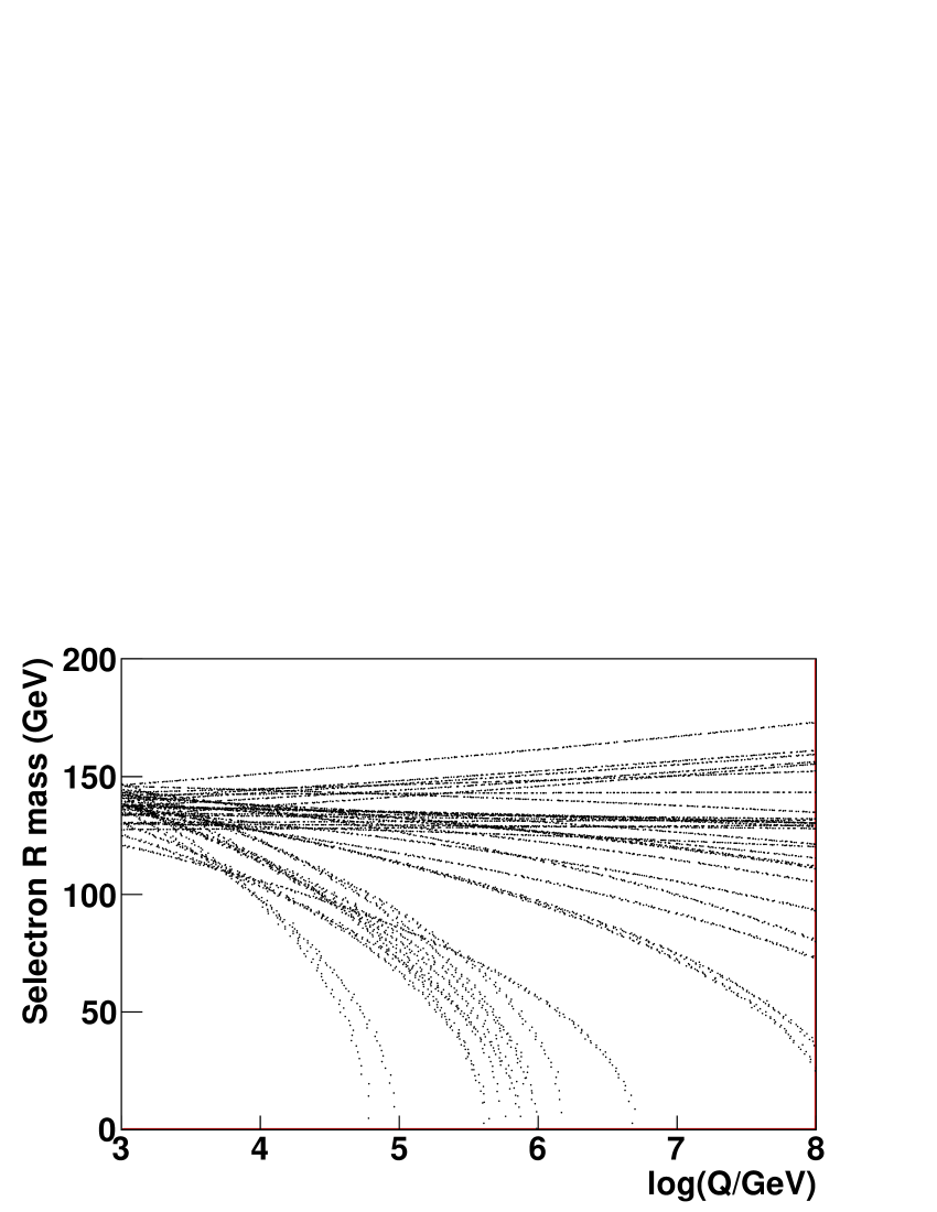
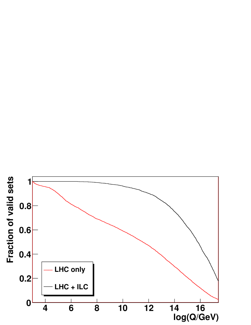
However, the errors are amplified strongly as function of the scale, especially in the scalar sector, at least for some parameters. This is to a large extent a manifestation of the “focus-point” phenomena in the MSSM focuspt : even if SPS1a does not correspond to what is usually referred as ’focus-point’ scenario in MSSM (which rather corresponds to much larger $m_{0}$ values), the focusing behavior is more general, i.e. in a large part of the MSSM parameter space the final (low scale) values of some of the scalar parameters (in particular $\mathrm{M}_{\mathrm{H}_{2}}$ driving the radiative electroweak symmetry breaking) are not very sensitive to the initial (high scale) input choice. This means that for the bottom-up direction even relatively small errors in some of the low scale parameters can result in large errors when evolved at high scale. Typically it was shown in Ref. Kneur:2008ur (Table X in Appendix B) that for relative uncertainties at the low electroweak scale of only 1% in the gluino mass $\mathrm{M}_{3}$ or the up-Higgs doublet mass term $\mathrm{M}_{\mathrm{H}_{2}}$ (letting all other parameters at their central SPS1a value), the RGE evolution up to the GUT scale amplifies the errors, resulting in relative uncertainties of 20-30% or even 100% on some of the final high scale soft mass parameters. The parameters entering $\mathrm{Tr}[Ym^{2}]$ are those particularly sensitive to this divergence behavior. Therefore, if the initial error is in the few percent range, some of the sfermion masses can become tachyonic well before reaching the final high scale. As an illustration Figure 1 (left) shows $\mathrm{M}_{\tilde{\mathrm{e}}_{\mathrm{R}}}$ as function of the logarithm of the scale for all parameter sets. $\mathrm{M}_{\tilde{\mathrm{e}}_{\mathrm{R}}}$ is particularly sensitive to the value of $\mathrm{Tr}[Ym^{2}]$, as deduced from Eq. 4. $\mathrm{Tr}[Ym^{2}]$ can deviate substantially from its nominal SPS1a value, e.g. from the largely undetermined $\mathrm{M}_{\tilde{\tau}_{\mathrm{L}}}$ in Table 5) for the LHC, and thus drive it to a tachyonic value well before the high scale is reached. A strong non-linear scalar mass dependence enters the RGEs of other scalar masses in addition to the $\mathrm{Tr}[Ym^{2}]$, such that some tachyonic masses may infect other scalar mass RGE. All sets which have at least one tachyonic parameter have to be removed. This necessity is also confirmed by the analysis of the covariance matrix of the parameters as function of the scale. If these tachyonic parameter sets are not removed, the covariance matrix can become singular.

Figure 1 (right) shows the percentage of valid non-tachyonic parameter sets. While at the LHC alone the percentage decreases immediately after the electroweak scale, the addition of the ILC stabilizes impressively the validity of the sets. For the LHC at 10¹² GeV only 30% of the parameter sets are still valid, whereas with the addition of the ILC 90% remain. At the unification scale for the LHC only 7% of the parameter sets remain, whereas for the LHC plus ILC measurements 38% remain valid, marking a clear improvement over the LHC alone. Similar results are obtained using SoftSUSY.

Once a real measurement is available, toy experiments will be defined around the central value of the measured data. In the following all confidence level definitions are defined with respect to valid, non-tachyonic parameter sets.

Given $N$ parameters for which the grand unification is to be tested, the following $\chi^{2}_{avg}$ is to be minimized for every scale:

$$\chi^{2}_{avg}(Q^{2})=\sum_{i,j}^{N}(\mathrm{M}_{i}-m_{U})(C_{p}^{-1})_{ij}(\mathrm{M}_{j}-m_{U})$$ (14)

where $C_{p}$ is the covariance matrix of the parameters and $\mathrm{M}_{j}$ the $j$-th mass parameter.

The scale where the $\chi^{2}_{avg}$ is minimal is the best-fit unification scale $Q_{U}$ and the parameter $m_{U}$ is the value of the unified parameter. As this procedure is applied to each dataset, the resulting distribution of all $m_{U}$ and $Q_{U}$ allow to read off the unification scale and unified parameter value as central values of their distributions and the error as RMS or Gaussian sigma of the distributions.

A closed formula can be derived for the parameter $m_{U}$ Schmelling:1994pz :

$$m_{U}(Q^{2})=\left(\sum_{i,j}(C_{p}^{-1})_{ij}\right)^{-1}\left(\sum_{i,j}(C_{p}^{-1})_{ij}M_{j}\right)$$ (15)

Figure 2: $\chi^{2}_{avg}$ of the unification calculation is shown as function of the scale for DS7. The minimum of the distribution is observed for a scale of about 10¹⁶ GeV as expected.

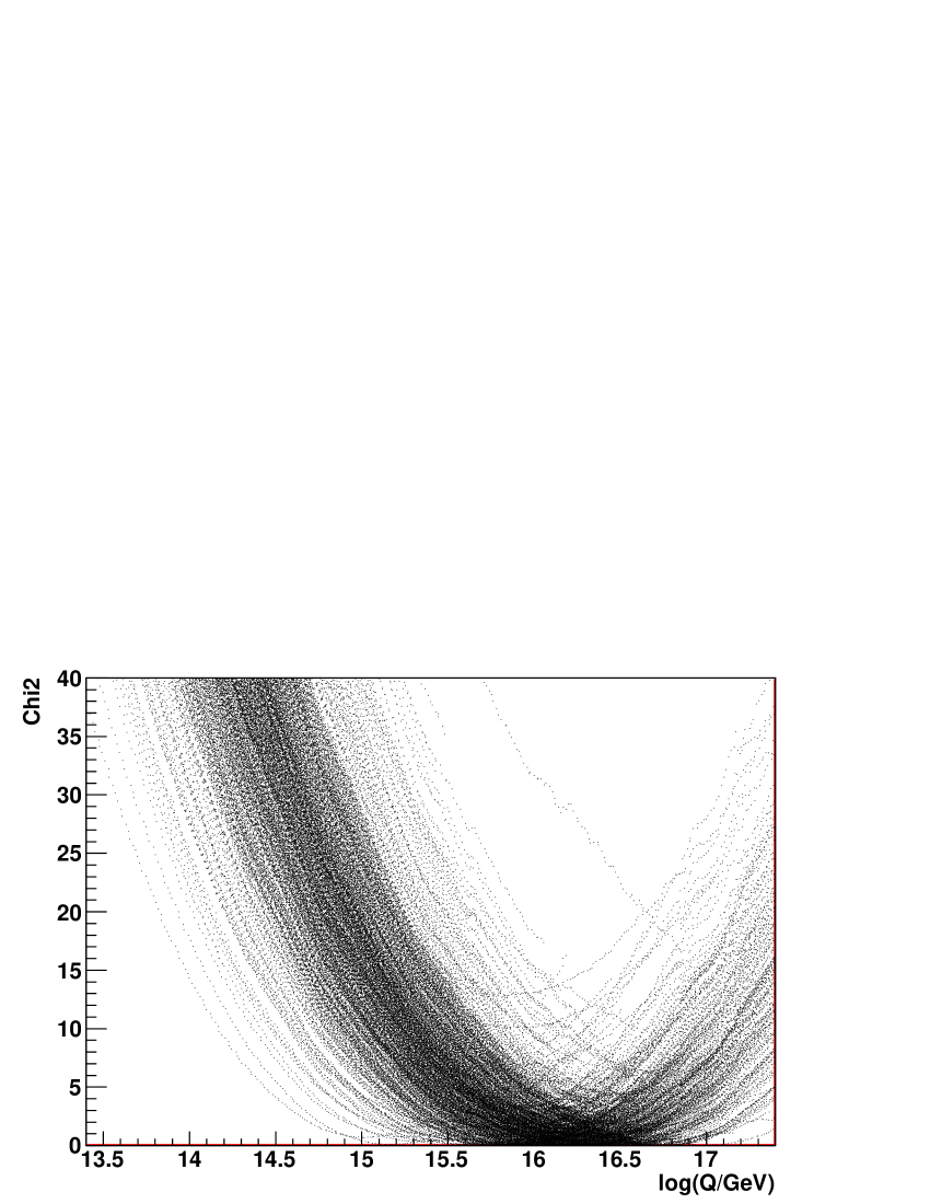
However this is not sufficient to claim grand unification as these calculations can also be performed for non-unifying parameters. To quantify the unification, the absolute value of $\chi^{2}_{avg}$ is used. The value is large when the $N$ parameters are not compatible with a unified one. It is small if the parameters are compatible. If $\chi^{2}_{avg}$ is smaller than a cut-off value ($\chi^{2}_{95}$), the dataset is unified. The cut-off is defined so that 95% of truly unifying datasets have a $\chi^{2}_{avg}$ value smaller than $\chi^{2}_{95}$. As an example the $\chi^{2}_{avg}$ for a sample of datasets is shown in Figure 2 as function of the scale (DS7). The minimum at a scale of about 10¹⁶ GeV is clearly visible.

5.2 Evolution of the parameters from LHC observables

In Table 5 the result of the determination of the MSSM parameters is shown in the first column for the LHC. Starting from these values the parameter sets are evolved individually to the high scale.

As noted before, at the LHC an eight-fold ambiguity will be observed. Therefore the first question is whether the RGE evolution of the eight solutions will result in similar or different patterns.

Figure 3: Evolution of the gaugino mass parameters to the GUT scale for DS7 (SPS1a).

Figure 4: Evolution of the gaugino mass parameters to the GUT scale for the ambiguous DS1, DS2, DS3 and DS10 at the LHC.

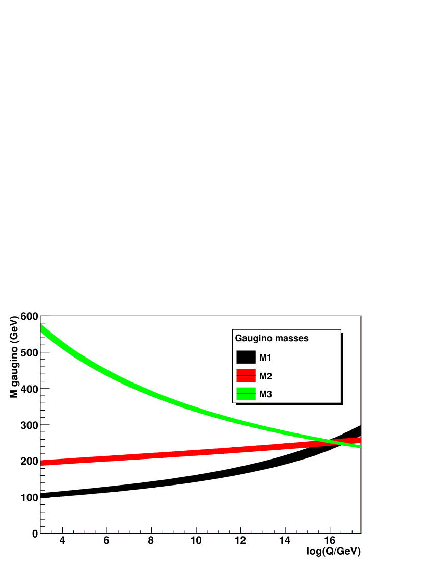
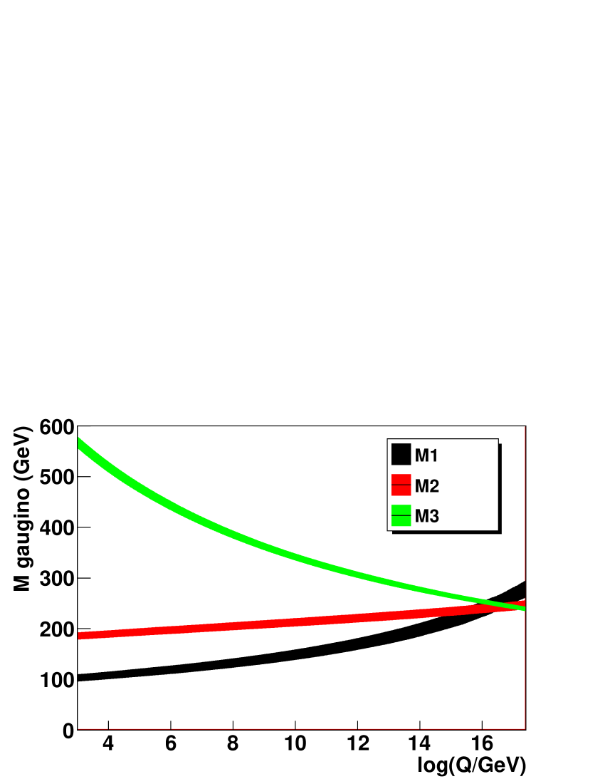
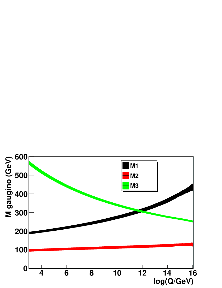
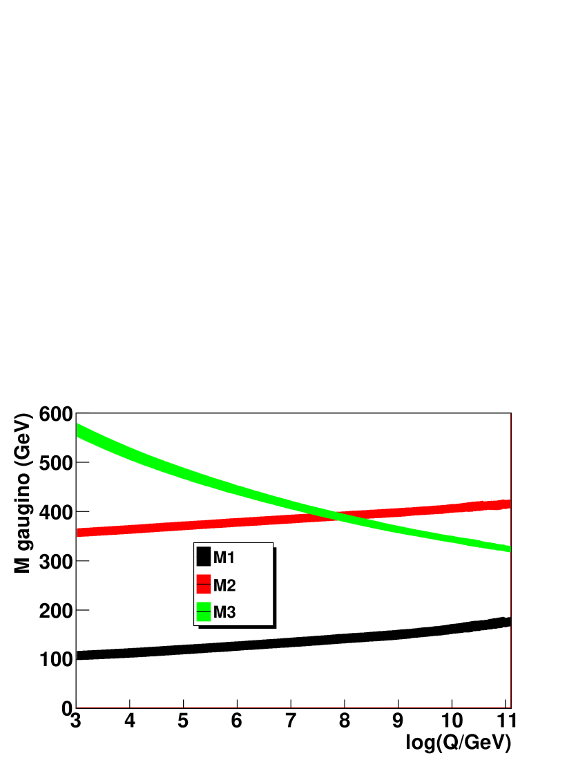
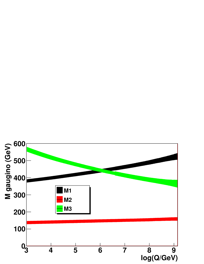
The evolution of the gaugino mass parameters is shown in Figure 4 for DS1, DS2, DS3 and DS10 and in Figure 3 for DS7 (SPS1a). The solutions DS8, DS9 and DS4 show the same pattern as DS2, DS3 and DS10, as expected, as only the sign of $\mu$ changes. In DS2 $\mathrm{M}_{1}$ and $\mathrm{M}_{2}$ are exchanged with respect to the correct solution. This leads to an intersection of $\mathrm{M}_{1}$ and $\mathrm{M}_{3}$ at $10^{12}$ GeV. In DS9 $\mathrm{M}_{3}$ intersects with $\mathrm{M}_{2}$ at about $10^{8}$ GeV, whereas in DS10 $\mathrm{M}_{3}$ and $\mathrm{M}_{1}$ intersect at $10^{6}$ GeV.

As expected the correct solution unifies the high scale. DS1, qualitatively at least, might unify. Thus six of the eight ambiguous solutions can be eliminated as candidates for unification. The difference between DS1 and the true solution being only the sign of $\mu$, it is natural that this solution is harder to distinguish from the correct one.

A comparison of the number of parameter sets compatible with a unified gaugino mass parameter of DS1 and DS7 is therefore necessary to quantify how well one will be able to distinguish the (non)-unification of these two solutions. For the true solution (DS7), at the unification scale determined for the gauginos, 95.4% of the toy experiments unify. In DS1 only 38% are unified. Thus the exclusion of unification for DS1 will indeed be very difficult at the LHC.

The results are in agreement with the expectation from the structure of the RGEs in the gaugino sector. The absolute value of the gaugino mass measured at the electroweak scale gives the starting point of the evolution, but the slope is essentially independent of the absolute value, so that a wrong parameter value at the electroweak scale cannot be compensated.

As two of the trilinear couplings are fixed at the LHC, no further information on the unification can be obtained from these parameters. The same is true for the third generation as the stop sector is not measured at the LHC. Therefore the study is restricted to the parameters of the first two generations.

Figure 5: Evolution of the first and second generation scalar mass parameters for the true solution (DS7) at the LHC : bottom-up evolution of the MSSM.

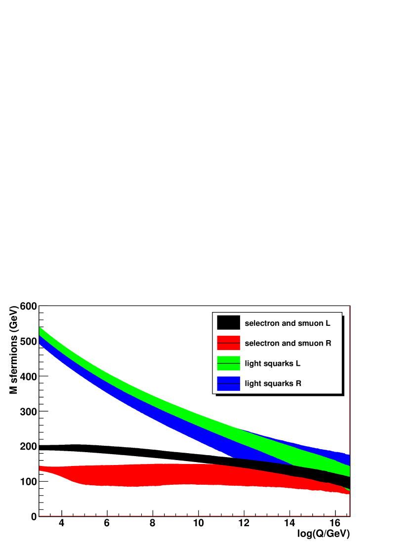
The bottom-up evolution of the scalar sector for the first two generations in DS7 is shown in Figure 5. The unification is qualitatively observed at about 10¹⁶ GeV as expected. While the slepton parameters are measured precisely at the electroweak scale, the coupling of the RGEs leads to a quick degradation of their precision as function of the scale. It is obvious that the scalars will not be able to improve the determination of the unification scale and therefore will not improve the separation of DS1 and DS7.

5.2.1 Unification scale and unified parameters

Given the observation of unification in the gaugino and scalar sector, the unification scale and the unified parameter can be determined at the LHC. Here the study is restricted to the true solution (DS7) without loss of generality, the solution of DS1 leads to a similar precision.

Name	Unified		Unification Scale		Parameter at
	Parameter		$[\log(Q/\mathrm{GeV})]$		1.7 $\cdot 10^{16}$ GeV
$\mathrm{m}_{1/2}$	251.9$\pm$	5.9	16.23$\pm$	0.29	252.3$\pm$	3.2
$\mathrm{m}_{0}$	98.5$\pm$	10.5	16.5$\pm$	0.6	100.8$\pm$	4.9

Table 6: Measurement of grand unification with LHC measurements (DS7). All masses are in GeV.

The results for the gaugino mass parameter $\mathrm{m}_{1/2}$ as well as the scalar mass parameter $\mathrm{m}_{0}$ are shown in Table 6. For the trilinear couplings the calculation is not useful as only one parameter is free ($\mathrm{A}_{t}$) and the other two are fixed at the electroweak scale.

The most precise determination of the unification scale is obtained in the gaugino sector with a measurement of $(1.7\pm 1.1)\cdot 10^{16}$ GeV. At the unification scale $\mathrm{m}_{1/2}$ is measured to about 2% and is in agreement with the nominal value of SPS1a (250 GeV). Fixing the scale reduces the error on the common mass parameter by almost a factor 2.

The common scalar parameter $\mathrm{m}_{0}$ is determined with a precision of about 10% in agreement with the nominal value of SPS1a of 100 GeV. As the scale is measured more precisely in the gaugino sector, combining the two sectors will not provide an improvement. Alternatively one can determine $\mathrm{m}_{0}$ at this fixed scale: $\mathrm{m}_{0}$ is measured to be 101 GeV with an error of 5 GeV, thus the error is reduced by a factor 2, not including the error on the scale determination.

Thus once the ambiguous solutions for the LHC are discarded, the common scalar and gaugino mass parameters can be reconstructed in a bottom–up approach with a precision of 10% and 2% respectively. The precision is improved to and 5% and 1% respectively if the unification scale is fixed. The fixed scale results can be compared to the mSUGRA parameter determination reported in Ref. Lafaye:2007vs where a precision of 2% was reached on the scalar mass and roughly 1% on the on the gaugino mass. Thus in the gaugino sector the results of top-down (mSUGRA) and bottom-up (MSSM) agree well, whereas in the scalar sector the determination bottom-up is less precise.

5.2.2 Effect of threshold corrections at the high scale

A further complication arises from threshold corrections of the unknown embedding theory. The size and the sign of such corrections are model-dependent, but in typical SU(5) models these primarily affect GUTthresh1 ; GUTthresh15 $\alpha_{S}(M_{GUT})$ (and $M_{GUT}$ to some extent). This could compensate for the observed mismatch, at two-loop RGE in MSSM, in $\alpha_{S}(M_{GUT})-\alpha_{2}(M_{GUT})\neq 0$ ($\alpha_{2}(M_{GUT})\equiv\alpha_{1}(M_{GUT})\equiv g^{2}_{1}/(4\pi)$). For a typical minimal SUGRA input, the latter mismatch is a few percent and negative (about -3% in particular for SPS1a). In addition, intrinsic corrections to the gaugino masses (i.e. corrections to Eq. 2) have been evaluated to be a few percent in a minimal SU(5) modelGUTthresh2 , i.e. roughly of the order of two-loop MSSM corrections, though the former can be much larger in non-minimal GUT models, e.g. with large representations of heavy chiral multiplets. Since specific GUT model corrections are anyway not implemented at present in the spectrum calculators, for simplicity a positive shift in $\mathrm{M}_{3}$ correlated with the $\alpha_{S}$ one (i.e. preserving Eq. 2 at one-loop) is assumed. The effect is thus approximated by shifting the measured parameter $\mathrm{M}_{3}$ by 3% for illustration, while possible model-dependent effects on other parameters are neglected.

The parameter $\mathrm{m}_{1/2}$, including the threshold corrections, is shifted by 3.5 GeV and the unification scale by 0.07, corresponding to a shift of $0.3\cdot 10^{16}$ GeV. The absolute values of the shifts have to be compared to the error of the determination of the common mass (5.9 GeV) and the scale (0.3). The shift corresponds to a deviation of less than half a standard deviation for the mass, thus the threshold effects will not play a large role at the LHC, given the expected precision.

In addition to the study of the central values, it is also interesting to address the question whether the threshold effects could lead to the conclusion that DS1 unifies and DS7 does not. The percentage of the unified parameter sets at the best scale is a good indicator. Including the threshold corrections, in DS7 the percentage drops to 87.4% (from 95.4%). In DS1, the unification percentage in the gaugino sector is 3% (from 38%). Thus the threshold corrections applied to DS1 will actually increase the difference between the true and the wrong solution. However, if the sign of the $\mathrm{M}_{3}$ shift is opposite (i.e. if the specific GUT model is such that those corrections are larger and essentially negative) this conclusion would change.

5.2.3 Evolution with shifted data

The studies described so far all dealt with datasets which are smeared, but centered around the true central value. An additional complication will arise with real data as the measured value of the parameters will be shifted, within the theoretical and experimental errors, from the true central value. In this case it is still possible to use the toy experiments but they are performed around the shifted values.

It is also necessary to verify that the theoretical errors used in the study cover at least the difference of the predictions from spectrum generators which have similar precision. The dataset (SPS1a) calculated by SUSPECT is used, but the MSSM parameters are determined by using SoftSUSY, i.e., SoftSUSY is used to predict the spectrum and evolve the parameters to the high scale. The SPS1a dataset from SUSPECT corresponds to a shifted dataset for SoftSUSY.

The common gaugino mass parameter $\mathrm{m}_{1/2}$ is determined to be $252.7\pm 6.4$ GeV at $\log(Q/\mathrm{GeV})=16.2\pm 0.3$ with SoftSUSY. The difference with respect to the determination using only SUSPECT is less than about one standard deviation (Table 6). In the scalar sector the common mass is determined to be 92 GeV with an error of 10 GeV. The results, both the central values and errors, at the EW scale as well as the GUT scale, are in excellent agreement with SUSPECT for the gaugino and scalar sector at the LHC.

It is also interesting to note that the percentage of toy sets compatible with grand unification in the gaugino sector is essentially unchanged: 95% for DS7, 35% for DS1.

The results show that as required by the definition of the size of the theoretical error at least the difference between different spectrum calculators is covered. While differences will be observed, depending on which calculator is used, the difference is small with respect to the expected error on the parameters and the unification scale.

5.2.4 High scale MSSM

To study the difference between bottom-up and top-down evolution, 5000 toy experiments are used to determine the parameters of the high scale MSSM. The results are compared to the parameters of the MSSM determination after their evolution to the high scale. Parameter sets are removed as soon as they became tachyonic. Thus they contribute to the RMS below the scale where they become tachyonic, but not above.

The precision of the parameters is comparable in the gaugino sector at the level of 20-30%. In the scalar sector the precision of the high scale MSSM parameters is reduced by a factor of more than 5. The difference with respect to the bottom-up evolution (Figure 5) is obvious in Figure 6.

Figure 6: Evolution of the first and second generation scalar mass parameters for the true solution (DS7) at the LHC : top-down evolution for the high scale MSSM.

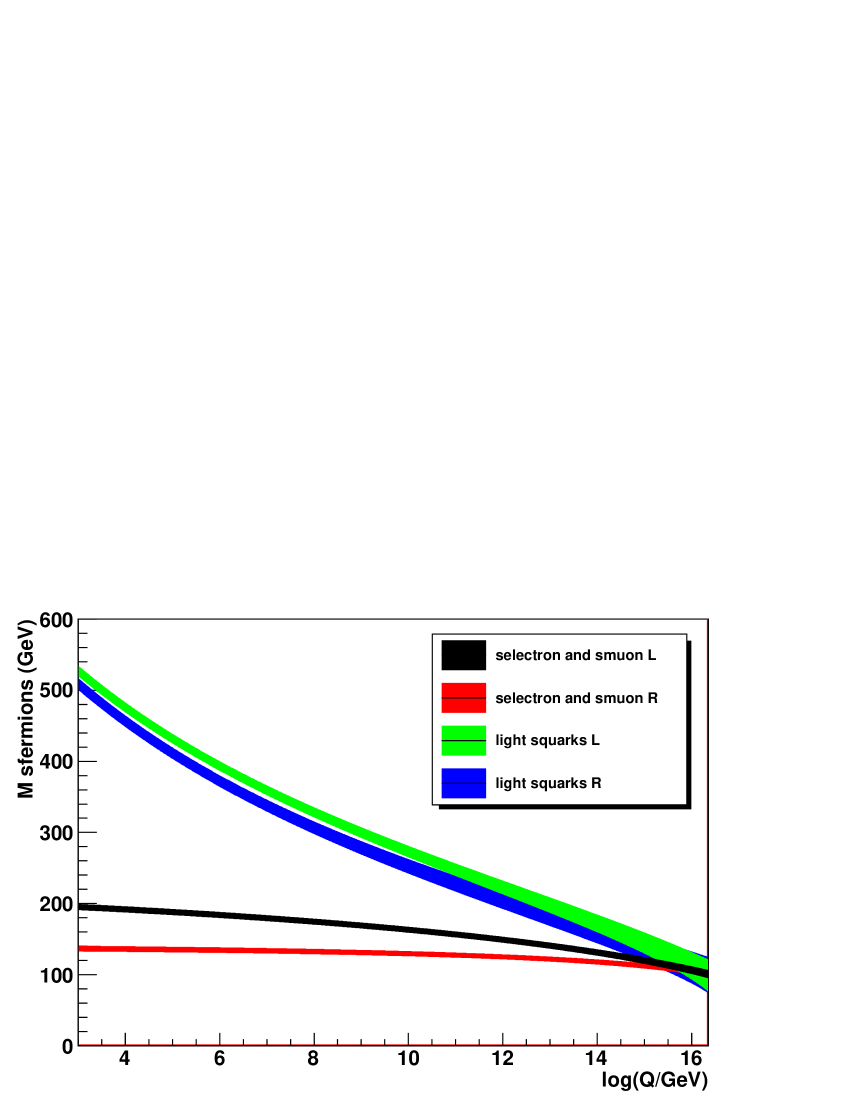
The apparent contradiction between the naive expectation that top-down should be equal to bottom-up and the large differences that are observed, can be traced to several factors: in contrast to the top-down evolution where all parameters are defined at a single high scale, in the bottom-up case initial conditions for the RGE are more sensitive to the (many) different physical scales. All threshold corrections are calculated at present in the one-loop approximation for most sparticles. This induces an increased sensitivity to the intrinsic errors.

In the stau sector only one measurement is available at the LHC. This measurement can be used to determine $\mathrm{M}_{\tilde{\tau}_{\mathrm{R}}}$. In the MSSM the parameter $\mathrm{M}_{\tilde{\tau}_{\mathrm{L}}}$ decouples and can take almost any value, even 1 TeV. This is reflected in the large error in Table 5. However, in the high scale MSSM, the top-down running introduces interdependencies. Keeping all parameters at their nominal SPS1a value and moving only $\mathrm{M}_{\tilde{\tau}_{\mathrm{L}}}$ to 200 GeV is not possible: the selectron and smuon masses are changed by 5 GeV. As the lepton-lepton edge, which depends on these slepton masses, is measured precisely at the LHC, such a large change is not compatible with the observables. Thus the high scale MSSM restricts the nominally available parameter space.

All scalar parameters are correlated non-linearly through $\mathrm{Tr}[Ym^{2}]$ entering all RGE equations. In a bottom-up evolution, large errors on the MSSM sfermion parameters induce a departure from zero in the boundary (initial) value of $\mathrm{Tr}[Ym^{2}]$Ṡince the dependence is quadratic, this is strongly amplified in the evolution. In the top-down evolution as the sfermion parameters are interdependent due to the RGEs and as a consequence all parameters are well measured, the departure of the $\mathrm{Tr}[Ym^{2}]$ from its SPS1a value is less pronounced and its effect smaller.

While the tachyonic parameter sets are removed and play no role at the high scale, they contribute to the error on the parameters at all scales below the GUT scale. These parameter sets are relatively far away from their nominal SPS1a value and thus lead to larger RMS for the parameters compared to the high scale MSSM where such parameter sets are excluded by construction.

5.3 Evolution of the parameters from LHC+ILC observables

In Table 5 the result of the determination of the MSSM parameters is shown in the third column for the combination of LHC and ILC. With the exception of the tri-linear couplings, the parameters are measured with excellent precision at the electroweak scale. Additionally the eight-fold ambiguity left by the LHC data alone is solved by the ILC.

Name	Unified		Unification Scale		Parameter at
	Parameter		$[\log(Q/\mathrm{GeV})]$		2.33 $\cdot 10^{16}$ GeV
$\mathrm{m}_{1/2}$	249.5$\pm$	1.8	16.37$\pm$	0.05	249.6$\pm$	1.5
$\mathrm{m}_{0}^{1/2\mathrm{Gen}}$	98.2$\pm$	10.7	16.5$\pm$	0.7	100.4$\pm$	2.5
$\mathrm{m}_{0}^{3\mathrm{Gen}}$	117.1$\pm$	27	15.4$\pm$	1.3	103.1$\pm$	25
$\mathrm{m}_{0}$	105.3$\pm$	9.1	15.9$\pm$	0.6	99.4$\pm$	2.0
$\mathrm{A}_{0}$	-164$\pm$	182	14.8$\pm$	4.5	-133.8$\pm$	207

Table 7: The results for the measurement of the common parameters and unification scale with LHC+ILC measurements in the bottom-up approach are shown. All masses are in GeV.

Figure 7: The evolution of the gaugino masses is shown for the combined results from LHC+ILC.

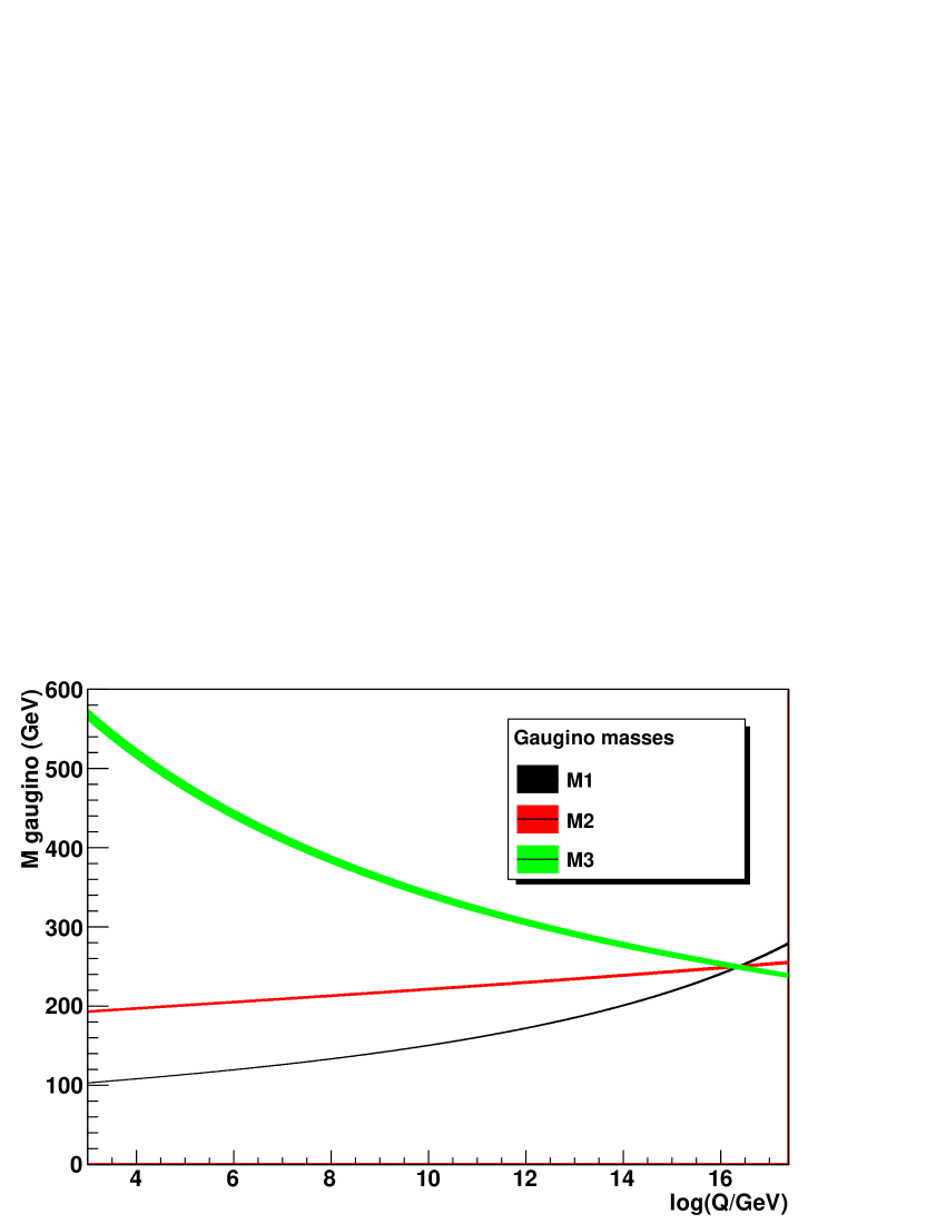
The results of the evolution of the parameters measured at the electroweak scale as well as the unification are shown in Table 7. The evolution of the three gaugino mass parameters is shown in Figure 7.

The common gaugino parameter $\mathrm{m}_{1/2}$ is determined with a precision of 1.8 GeV at a grand unification scale of $(2.33\pm 0.28)\cdot 10^{16}$ GeV in agreement with the SPS1a parameter set definition. Note that while the logarithm of the unification scale is determined with a precision of 0.3%, due to the proper error propagation, the scale in GeV is only determined with 10% precision. The error with respect to LHC alone is reduced by a factor 3.

Fixing the unification scale to the central value determined by the gauginos, the error on $\mathrm{m}_{1/2}$ would be reduced by about 0.2 GeV. It is also instructive to analyze the individual contributions of the three parameters to the determination of the unified mass parameter. At the unification scale $\mathrm{M}_{1}$, $\mathrm{M}_{2}$ and $\mathrm{M}_{3}$ are measured with a precision of 1.6 GeV, 2.0 GeV and 3.3 GeV respectively. Thus the error on $\mathrm{m}_{1/2}$ is essentially equal to the precision of $\mathrm{M}_{1}$. The naive combination of the three parameter errors, i.e., ignoring correlations, would lead to an error of 1.1 GeV, almost 30% better than that obtained. While $\mathrm{M}_{3}$ is uncorrelated with the other two parameters, $\mathrm{M}_{1}$ and $\mathrm{M}_{2}$ are almost 100% positively correlated. Thus combining the latter two will not increase the precision. $\mathrm{M}_{3}$ on the other hand, while not correlated, is less precisely measured and therefore the combined error is decreased only by a small amount in the combination as the error ($\sigma$) on the combination of two uncorrelated measurements ($\sigma_{1}$, $\sigma_{2}$) reads:

$$\sigma=1/\sqrt{1/\sigma_{1}^{2}+1/\sigma_{2}^{2}}$$ (16)

Figure 8: The evolution of the scalar masses of the first generation is is shown for the combined results from LHC+ILC.

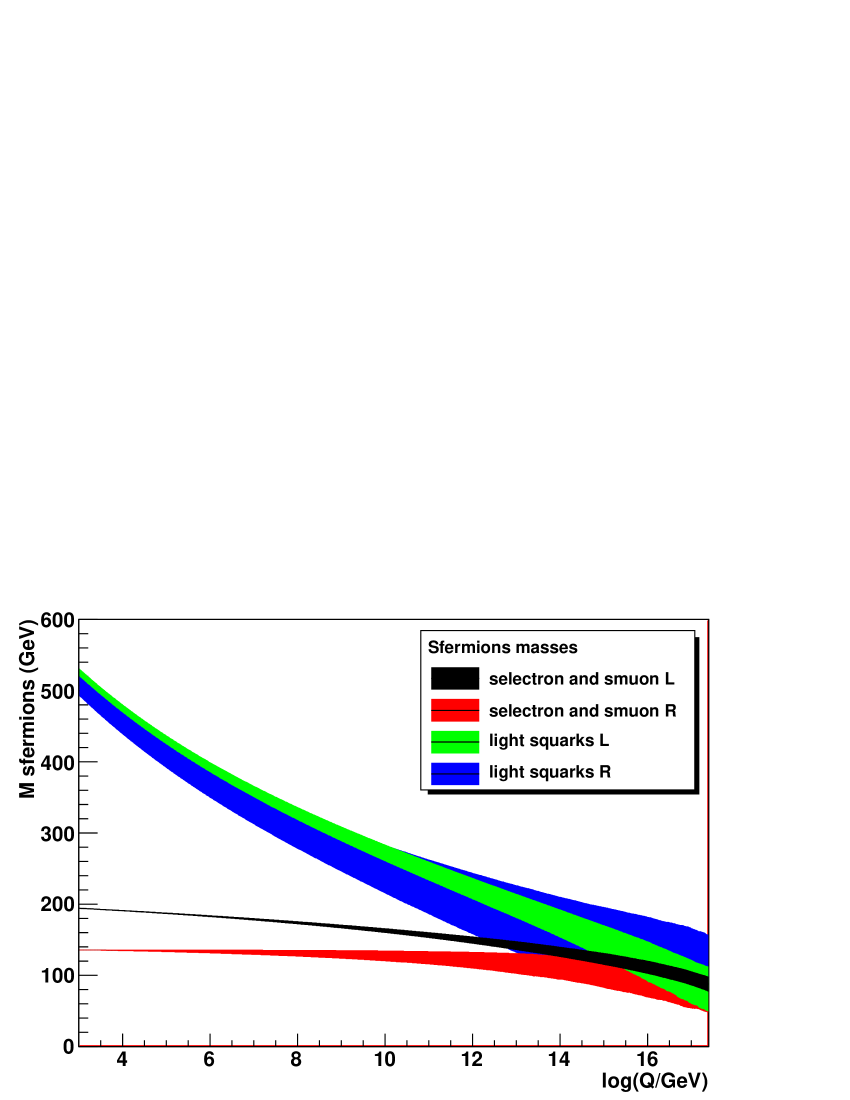
Due to the increased precision of LHC+ILC, the unification of the scalar mass parameters can be separated into the first two generations and the 3rd generation. The evolution of the scalar masses of the first generation is shown in Figure 8. As shown in Table 7, $\mathrm{m}_{0}^{1/2\mathrm{Gen}}$ can be determined with a precision of about 10% in agreement with the nominal value (100 GeV) of SPS1a. The determination of the logarithm of unification scale is less precise than the precision in the gaugino sector by an order of magnitude. Using the unification scale defined by the gaugino measurement, the error is reduced to 2.5 GeV. It is interesting to note that in the scalar case the naive combination of the parameters neglecting the covariance matrix would lead to an error on $m_{0}^{1/2Gen}$ of 8.2 GeV, thus greater than the correct value. This is due to the large negative correlations among the parameters which reduce the total error.

Figure 9: The evolution of the scalar parameters of the third generation is shown for the combined results from LHC+ILC as function of the logarithm of the scale.

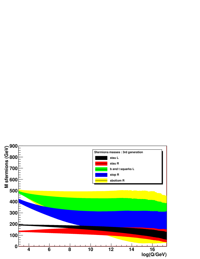
For the 3rd generation the unification procedure leads to a less precise determination (27 GeV) of the common scalar parameter as can be immediately inferred from Figure 9 as well as Table 7. The improvement by fixing the unification is rather small. The larger errors with respect to the first two generations are due to two sources. The parameters of the third generations are less precisely measured than those of the first two generations. Additionally, as discussed in Section 2.1 the sfermion mass terms in the RGE have a stronger inter-dependence. Nevertheless the reconstructed unification scale is in agreement with the SPS1a parameter set.

If instead of separating the first and second generation from the third generation (and the two Higgs parameters), all parameters relating to scalars are combined, the error on the determination of the unification scale as well the parameter is decreased as shown in the second to last row of Table 7. Using the central value of the unification scale determined by the gaugino sector, the error on $\mathrm{m}_{0}$ is reduced to 2 GeV. This error is smaller than the naive combination ignoring correlations by a factor 3, showing the necessity of a proper treatment of the errors and correlations.

It is interesting to note that the error here is identical to the error from the LHC alone. This might seem surprising at first sight as the slepton sector is measured experimentally an order of magnitude more precisely at the ILC than at the LHC. The reason for this (superficial) lack of impact lies again in the structure of the RGEs. The error on the sleptons, as shown in Figure 8, increases strongly as function of the scale due to the coupling with the less precisely determined squark sector. Thus at the unification scale, the slepton precision of the ILC is diluted by the LHC squark precision. Additionally while for the combination of LHC and ILC no MSSM parameters are fixed, for the LHC the trilinear couplings of the sbottoms and staus are fixed. Fixing these leads to contraction of the allowed parameter space and therefore an artificial decrease of the scalar mass error at the LHC.

Figure 10: (left) The evolution of the trilinear parameters of the third generation is shown for the combined results from LHC+ILC. (right) The evolution of the squares of the Higgs sector parameters $\mathrm{M}_{\mathrm{H}_{1}}$ and $\mathrm{M}_{\mathrm{H}_{2}}$ is shown for LHC+ILC.

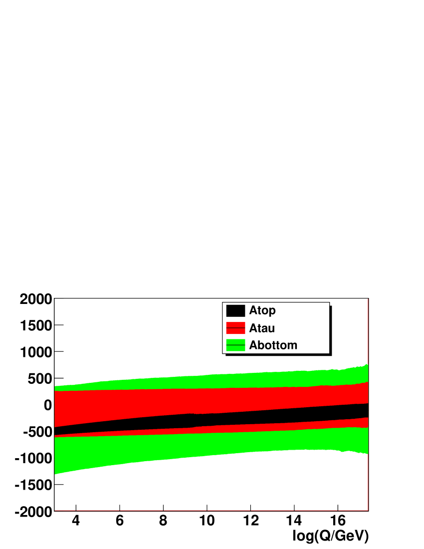
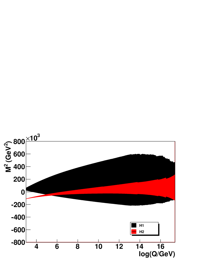
Of the trilinear couplings, only $\mathrm{A}_{t}$ can be measured with good precision with the mass measurements from the ILC and the edges from the LHC. Further measurements will be necessary to constrain these parameters. For completeness sake the results are shown in the last line of Table 7 and in Figure 10 (left). Due to the large errors on the parameters determined at the electroweak scale, the parameters are compatible with unification at all scales. Fixing the unification scale to the one determined by the gaugino sector, the error on $\mathrm{A}_{0}$ is 200 GeV. This is a slight improvement compared to the error of 211 GeV on $\mathrm{A}_{t}$ at the unification scale. Only $\mathrm{A}_{\tau}$ contributes to the reduction of the error as $\mathrm{A}_{b}$ has a larger error and is therefore irrelevant for the combination.

The evolution of the squares of the Higgs sector parameters $\mathrm{M}_{\mathrm{H}_{1}}$ and $\mathrm{M}_{\mathrm{H}_{2}}$, replacing the electroweak parameters $m_{A}$ and $\mu$ is shown in Figure 10 (right). The square of $\mathrm{M}_{\mathrm{H}_{2}}$ is negative at the electroweak scale, as required by electroweak symmetry breaking, and reasonably well determined. As the evolution proceeds to higher scales, the error increases significantly, somewhat faster for $\mathrm{M}_{\mathrm{H}_{1}}$. At the high scale the parameters are compatible with the true value of $(100~{}\mathrm{GeV})^{2}$, but also with zero. Thus there is no significant contribution on the determination of $\mathrm{m}_{0}$ from these parameters.

The fixed scale results of the common parameters at the high scale can be compared to the mSUGRA parameter determination reported in Ref. Lafaye:2007vs . While for the gauginos the error of the bottom-up determination compared to mSUGRA is about 2.5 times larger, the common scalar mass is determined with a precision 5 times better in mSUGRA. The largest difference is observed for the tri-linear coupling where the mSUGRA determination is more precise than the bottom-up one by a factor of 20. This shows that bottom-up and top-down do not lead to the same results.

The last question to be addressed is to determine the probability with which grand unification will be measured in the four measurements. At the unification scale 95% of the toy experiments show unification in the gaugino sector in agreement with the definition of the $\chi^{2}$ cut. For the scalar parameters at the unification scale defined by the gauginos, the most precise measurement of this scale, 90% unify. For the trilinear couplings 93% of the toy experiments are compatible with grand unification.

The additional observables added by the ILC to the LHC dataset indeed increase the precision of the determination of the couplings in the gaugino sector by a large factor. Additionally different unification hypotheses can be tested (full scalar unification, separate unification for the light and heavy generations).

5.3.1 Effect of threshold corrections at the high scale

To study the effect of threshold corrections the measured value of $\mathrm{M}_{3}$ is shifted by 3% as in Section 5.2.2. The common gaugino mass is then determined to be 251.7 GeV and the scale is shifted by 0.05. The mass shift at the LHC alone is less than about half of a sigma. Due to the higher precision of the combination LHC+ILC, the shifts, while similar in absolute numbers, is now of the order of a sigma.

The effect on the percentage of unifying parameter sets is also much larger: it decreases from 95% to 77%. For comparison, the effect is only half as large for the LHC alone. The increased precision added by the ILC means that the effect of threshold effects become more important.

5.3.2 Evolution with shifted data

As in Section 5.2.3 to illustrate the effect of a shifted dataset, the central values from SUSPECT are used, but the predictions as well as the evolution bottom-up are performed by SoftSUSY.

In the gaugino sector the unification scale is determined with the same precision as before. The central values differ by less than 0.01, corresponding to one fifth of a sigma. $\mathrm{m}_{1/2}$  is determined to be 249.5 GeV, in excellent agreement with the determination using SUSPECT. The error on $\mathrm{m}_{1/2}$ is comparable at 1.6 GeV. 94% of the parameter sets unify.

In the scalar sector $\mathrm{m}_{0}$ is shifted by 1.6 GeV closer to the nominal value of SPS1a. The error from the determination of 9 GeV is comparable to that from SUSPECT. Thus the shift is less than one fifth of a sigma.

The study shows that the theoretical errors fulfill the requirement that they cover at least the difference between different calculations of the spectrum and the RGE running. The results are in excellent agreement, showing that the analysis is robust.

5.3.3 High scale MSSM

As shown in Figure 1 (right), the fraction of “non-tachyonic” datasets is much higher in the LHC+ILC case. But the comparison of the errors on the MSSM parameters evolved to the high scale with the high scale MSSM parameters shows again the difference between a top-down and a bottom-up approach. The difference between the errors on the parameter determination at the unification scale is reduced due to the increased precision added by the ILC measurements. In the gaugino sector these are now of the order of 10-20%. In the scalar sector the differences remain much larger, a factor 5 in the stau sector for example. The results of the top-down evolution shown in Figure 11 can easily be compared with the bottom-up evolution shown in Figure 10 (right) and Figure 9.

Figure 11: The top-down evolution of high-scale MSSM parameters at the LHC+ILC is shown for : (left) third generation scalar mass parameters, (right) squares of the Higgs sector parameters $\mathrm{M}_{\mathrm{H}_{1}}$ and $\mathrm{M}_{\mathrm{H}_{2}}$.

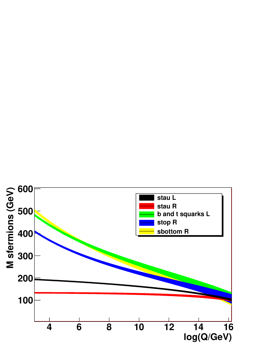
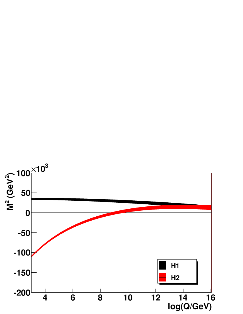
The strong sensitivity to the Higgs mass term $\mathrm{M}_{\mathrm{H}_{2}}$  as illustrated in Figure 11, is not surprising since in most MSSM scenario its evolution, mainly driven by the top Yukawa coupling, drastically accelerates near the EW scale, where generally $\mathrm{M}_{\mathrm{H}_{2}}^{2}$ changes sign. In other words the slope of its beta function becomes large around the EW breaking scale, which is taken as the initial scale in a bottom-up evolution. Therefore in the bottom-up evolution even a small error in the initial low scale $\mathrm{M}_{\mathrm{H}_{2}}$ value can induce a very large difference at the high scale. In contrast, in a top-down evolution near the GUT scale the initial slope of the beta function for $\mathrm{M}_{\mathrm{H}_{2}}$ is moderate, and the final value at the EW scale is less dependent on initial high scale boundary conditions, illustrating a typical focusing behavior.

To illustrate the impact of this behavior on the scalar mass determination, a bottom-up parameter set is selected for which $\mathrm{M}_{\tilde{\mathrm{e}}_{\mathrm{R}}}$, after evolution to the high scale, is about 60 GeV, i.e., far away from the SPS1a nominal values. The choice of $\mathrm{M}_{\tilde{\mathrm{e}}_{\mathrm{R}}}$ to select the dataset/parameter set is motivated by the fact that it is well measured and $\mathrm{M}_{\tilde{\mathrm{e}}_{\mathrm{R}}}$ is the lightest scalar mass. This parameter is therefore more likely to evolve to tachyon values in a bottom-up evolution. A different choice of the scalar parameter departing from its SPS1a value would also have been possible.

Two high scale MSSM parameter determinations are performed with this dataset: one starting from the nominal SPS1a values and a second one starting from the MSSM results after evolution to the high scale. In the first case, the high scale MSSM scalar masses are determined at values within 2 GeV of the SPS1a nominal values for the slepton masses. The best-fit result of the second determination is compatible with the result of the bottom-up study, where apart from $\mathrm{M}_{\tilde{\mathrm{e}}_{\mathrm{R}}}$ other scalar masses are also far away from their nominal SPS1a values at the high scale.

The $\chi^{2}$ of both parameter determinations is very good, less than the degrees of freedom with a slightly smaller value for the MSSM bottom-up result ($\Delta\chi^{2}=3/18$d.o.f.). The result of the evolution of the two high scale MSSM determinations is shown in Figure 12 for the third generation scalar parameters and $\mathrm{M}_{\mathrm{H}_{2}}$. All parameters with the exception of $\mathrm{M}_{\tilde{\mathrm{t}}_{\mathrm{R}}}$ and $\mathrm{M}_{{\tilde{\mathrm{q}}3}_{\mathrm{L}}}$ (and the tri-linear couplings) converge from extremely different values at the high scale to the same value at the EW scale. This effect can be understood from the fact that at the leading one-loop RGE, both $\mathrm{M}_{\tilde{\mathrm{t}}_{\mathrm{R}}}$ and $\mathrm{M}_{{\tilde{\mathrm{q}}3}_{\mathrm{L}}}$ evolution depend strongly on $\mathrm{M}_{\mathrm{H}_{2}}$, which exhibits a strong variation around the EW scale as mentioned above. In contrast, other relevant scalar masses do not depend (at one-loop RGE level) on $\mathrm{M}_{\mathrm{H}_{2}}$. Moreover the other scalar parameters RGE depend very little on $\mathrm{M}_{\tilde{\mathrm{t}}_{\mathrm{R}}}$ and $\mathrm{M}_{{\tilde{\mathrm{q}}3}_{\mathrm{L}}}$, the effect is suppressed by the bottom Yukawa coupling, which is quite small for SPS1a. Indeed, the evolution of the combination $2\cdot\mathrm{M}_{{\tilde{\mathrm{q}}3}_{\mathrm{L}}}^{2}-\mathrm{M}_{\tilde{\mathrm{t}}_{\mathrm{R}}}^{2}$, which eliminates the dominant dependence on $\mathrm{M}_{\mathrm{H}_{2}}$ at one–loop RGE, has essentially the same form for the two solutions as expected.

Figure 12: The top-down evolution of high-scale MSSM parameters at the LHC+ILC is shown for : (left) third generation scalar mass parameters, (right) squares of the Higgs sector parameters $\mathrm{M}_{\mathrm{H}_{1}}$ and $\mathrm{M}_{\mathrm{H}_{2}}$. The two lines for each parameter correspond to the two essentially degenerate solution for the same dataset. One solution is close to the SPS1a values at the high scale, the other one far away. At the EW scale the mass parameters with the exception of $\mathrm{M}_{\tilde{\mathrm{t}}_{\mathrm{R}}}$ and $\mathrm{M}_{{\tilde{\mathrm{q}}3}_{\mathrm{L}}}$ converge to the same value.

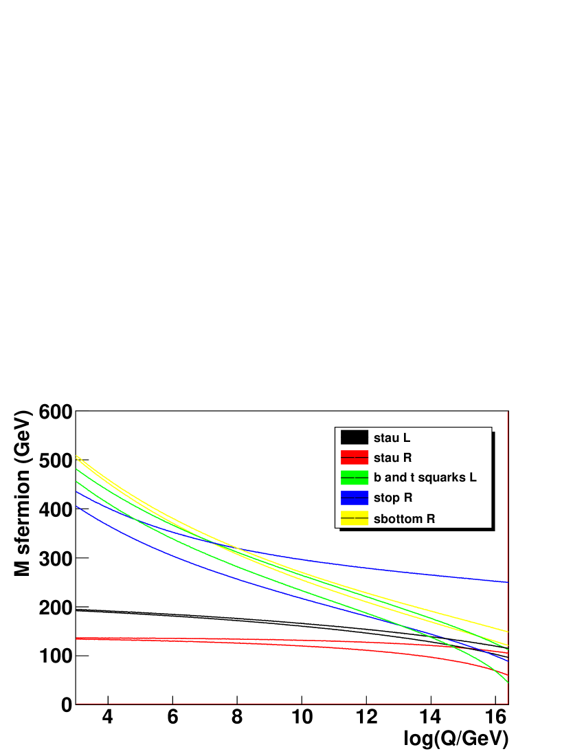
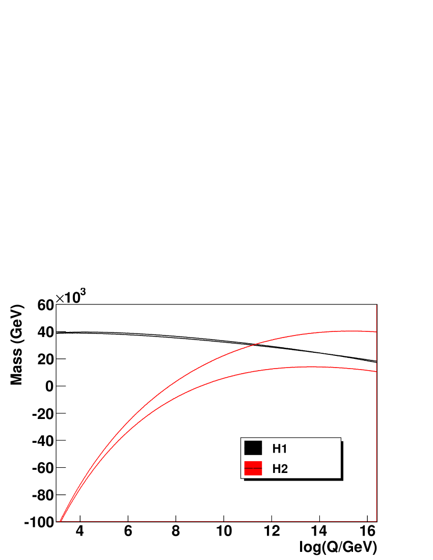
Given the smallness of $\Delta\chi^{2}$, the two solutions are de facto degenerate. It is interesting to ask why the bottom-up solution has found an ever so slightly better solution than the standard high scale study. While at the EW scale the difference of $\mathrm{M}_{\tilde{\mathrm{t}}_{\mathrm{R}}}$ and $\mathrm{M}_{{\tilde{\mathrm{q}}3}_{\mathrm{L}}}$ for the two solutions is of the order of 20 GeV, i.e., close by, at the high scale the difference is of the order of 150 GeV. Thus at the EW scale the sampling of the parameter space is much easier: all mass parameters but two are the same and only a small excursion of 20 GeV in $\mathrm{M}_{\tilde{\mathrm{t}}_{\mathrm{R}}}$ and $\mathrm{M}_{{\tilde{\mathrm{q}}3}_{\mathrm{L}}}$ is needed to find and differentiate between the two solutions. At the high scale however, all scalar parameters of the two solutions are far apart: 60GeV for $\mathrm{M}_{\tilde{\mathrm{e}}_{\mathrm{R}}}$, 150 GeV for $\mathrm{M}_{\tilde{\mathrm{t}}_{\mathrm{R}}}$ etc. Therefore the parameter determination will find easily the solution close to the values of SPS1a, while it is more difficult to find the second solution as a much larger parameter space has to be sampled. But even in this case, by construction, the top-down extrapolation will miss the contribution of the tachyonic parameter sets from the bottom-up approach.

The high scale MSSM top-down results presented in this study agree with the bottom-up results presented by other groups Allanach:2004ud ; Bechtle:2005vt . In Refs. Allanach:2004ud ; Bechtle:2005vt additional ILC observables are used (polarized cross sections) and the theory errors are set to zero. Additionally in Ref. Allanach:2004ud the trilinear parameters $\mathrm{A}_{\tau}$ and $\mathrm{A}_{b}$ are required to be at the high scale compatible with $\mathrm{A}_{t}$ within 2 sigma. This additional requirement leads mechanically to a reduction of the error on the corresponding mass parameters.

6 Conclusions

The discovery of supersymmetry at the LHC will lead to a wealth of signatures which can be exploited to determine many MSSM parameters. In parameter regions similar to the SPS1a parameter point, they can be determined at the LHC up to an at least 8-fold ambiguity in the gaugino sector. Although a part of those ambiguities may be resolved, e.g., by a complementary study of the MSSM contributions to the dark matter relic density, a full resolution will likely require a complete observation of the sparticle spectrum at the ILC.

Starting from the electroweak scale, we can test the unification of different supersymmetry-breaking parameters. While remaining ambiguities make it impossible to measure unification at the LHC, it will nonetheless be possible to classify solutions into the ones compatible and the ones not compatible with unification. In the case of an ambiguous solution (DS1) which differs from the true solution only by the sign of $\mu$, the differentiation will be difficult as about 38% of the parameter sets corresponding to this wrong solution nevertheless unify.

This way, at the LHC the unified gaugino mass parameter can be measured bottom-up to about 2% and the logarithm of the unification scale to 1.7%. Adding the ILC data improves the determination of the mass by more than a factor 3 and the unification scale by almost one order of magnitude. In the scalar sector the errors are generically larger at the level of 10%. The errors on the trilinear couplings are too large to be used for a determination of the unification scale.

The robustness of our results we have confirmed by comparing two different renormalization group tools: SUSPECT and SoftSUSY. The parameter determination as well the evolution are in good agreement within the errors. Threshold corrections at the high scale were studied for a particular model, motivated by SU(5) grand unification. The percentage of parameter sets unifying is affected more strongly including the ILC observables providing an increased sensitivity.

Finally, our study show that a proper bottom-up approach will clearly lead to different results from simply determining the parameters of the high scale MSSM (or mSUGRA). In addition to resolving the ambiguities at the LHC, the ILC plays a strong role in the stabilization of the validity of the parameter sets as function of the scale.