Multielectron corrections in molecular high-order harmonic generation for different formulations of the strong-field approximation

Abstract

We make a detailed assessment of which form of the dipole operator to use in calculating high order harmonic generation within the framework of the strong field approximation, and look specifically at the role the form plays in the inclusion of multielectron effects perturbatively with regard to the contributions of the highest occupied molecular orbital. We focus on how these corrections affect the high-order harmonic spectra from aligned homonuclear and heteronuclear molecules, exemplified by $\mathrm{N}_{2}$ and CO, respectively, which are isoelectronic. We find that the velocity form incorrectly finds zero static dipole moment in heteronuclear molecules. In contrast, the length form of the dipole operator leads to the physically expected non-vanishing expectation value for the dipole operator in this case. Furthermore, the so called “overlap” integrals, in which the dipole matrix element is computed using wavefunctions at different centers in the molecule, are prominent in the first-order multielectron corrections for the velocity form, and should not be ignored. Finally, inclusion of the multielectron corrections has very little effect on the spectrum. This suggests that relaxation, excitation and the dynamic motion of the core are important in order to describe multielectron effects in molecular high-order high harmonic generation.

I Introduction

High harmonic generation can be used for attosecond imaging of molecules Smirnova . This is a consequence of the fact that the structure of an aligned molecule can be inferred from quantum-interference patterns, which appear in the high-harmonic spectra. Understood in terms of the three-step model, in which an electron reaches the continuum by tunneling or multiphoton ionization, is accelerated by the field and subsequently recombines with a bound state of its parent molecule, emitting a high-order harmonic photon Lewenstein , this phenomenon occurs due to the electron returning to different spatially separated centers. The simplest scenario is high-harmonic generation in a diatomic molecule, for which, in principle, recombination and thus high-harmonic emission can take place from either atomic center. This is a microscopic equivalent to the double slit experiment doubleslit .

How to accurately describe the whole process of high harmonic generation (HHG) in molecules is still an open problem. There are two main theoretical approaches that can be used. Firstly one can attempt a fully numerical solution by using density functional theory, which gives accurate results but inhibits a more complete understanding of the process tddft . Secondly, one can employ the traditional atomic three step model, within the strong-field approximation Lewenstein , and calculate the molecular bound-state wavefunctions using a quantum chemistry code GAMESS . In this framework, the bound states of the molecule are mainly incorporated in the ionization and recombination steps, in the form of prefactors. The latter approach allows a better physical understanding of the problem. The price one pays, however, is that, in order to be able to treat HHG within a semi-analytical framework, several approximations must be made.

It is well known that the harmonic spectrum is proportional to the modulus squared of the Fourier transform of the dipole acceleration. By using the Ehrenfest theorem the dipole acceleration can be replaced by the dipole velocity or the dipole length, with no loss of accuracy so long as the integration is over all time and no physical approximations are made upon all wavefunctions involved. However, when the SFA is used, this is no longer the case, and replacement of the dipole operator gives rise to inconsistencies in the SFA dipole matrix elements, which vary depending on the form of the operator used. The most well known of these is the lack of translational invariance when using the length form of the dipole operator. In the single-active electron approximation, it has been shown that the velocity form gives the most reliable results JMOCL2007 and is easier to use than the acceleration form.

In calculating the SFA prefactors the simplest approach is to use the highest occupied molecular orbital (HOMO) Milosevic . However, the problems that arise in this case are 1) which orbitals have the predominant influence on high harmonic generation and 2) how to accurately include the multielectron effects of electron exchange and correlation.

The first problem has to some extent been addressed in Ref. Smirnova by noting that the ionization potential of different orbitals varies with the rotation of the molecule and hence the corresponding cutoffs in the high harmonic spectra will be different. Furthermore, the symmetry of the orbital will strongly affect the contribution of specific orbitals to high-order harmonic spectra. This is particularly true as the alignment angle of the molecule with respect to the laser-field polarization varies. In previous work CarlaBrad we also investigated high-order harmonic generation beyond the single-active orbital approximation. In particular, we addressed the quantum interference between the HOMO and the HOMO-1 of $\mathrm{N}_{2}$ and the HOMO and the lowest unoccupied molecular orbital (LUMO) of $\mathrm{N}_{2}^{+}$. For the latter case, we have also observed that electron recombination to different orbitals can be mapped into different cutoffs in the HHG spectra. Our investigations, however, did not incorporate electron correlation. In fact, we have either dealt with simplified multielectron models, in which the time evolution of the optically active electrons has been decoupled, or with a coherent superposition of one-electron states.

The second problem is what we propose to investigate in this paper and in doing so to consider the influence that these multielectron effects have on high harmonic generation. In particular, we wish to incorporate such effects perturbatively around the contributions of the highest occupied molecular orbital. Although correlation in molecular high-order harmonic generation has been addressed in Refs. Patchkovskii ; Smirnova , utilizing a multielectron version of the strong-field approximation, such studies have been performed numerically to a great extent. Including the correlation analytically in the dipole matrix elements facilitates more insight into the effects that correlation has on the high harmonic spectra. In Ref. Santra , many-body perturbation theory was used to include electron correlation as corrections to the standard three step model. Therein, however, only the response of single atoms has been addressed.

From the viewpoint of which form of the dipole operator to use, we are particularly interested in how such corrections are affected by the different formulations, especially in molecular targets. Indeed, even in the single-active electron approximation, the discrepant results obtained for each dipole form have raised considerable debate. By extending the debate to multielectron effects in molecules, more insight into which operator is most accurate for harmonic generation, and indeed all strong field phenomena, is gained. The use of molecules is beneficial because the two-center interference pattern gives another indicator of how the formulation is performing.

In order to make such an assessment, we will employ many-body perturbation theory along the lines of Ref. Santra and the dipole moment in its length and velocity forms. For that purpose, we will consider two isoelectronic molecules: $\mathrm{N}_{2}$ and CO. The HOMO, LUMO and HOMO-1 in both molecules have similar geometry. The main difference between them is that $\mathrm{N}_{2}$ is a homonuclear molecule, while CO is heteronuclear. This means that, for the latter molecule, there is an intrinsic static dipole moment. According to Ref. Santra , one expects the multielectron corrections to be more prominent in this case.

This work is organized as follows. In Sec. II, we provide the theoretical framework which we will employ in order to compute the high-order harmonic spectra. We then calculate the transition amplitudes, in different formulations (Sec. II.1), within the strong field approximation, and calculate the multielectron corrections (Sec. II.2), with particular focus on the form of the dipole operator. Subsequently, in Sec. III, these expressions are employed to compute the high-harmonic spectra. Finally, the paper is summarized in Sec. IV. Atomic units are used throughout.

II Theory

II.1 Transition amplitude

The SFA transition amplitude in the particular formulation of Ref. Lewenstein reads

$$b_{\Omega} = i\int_{-\infty}^{\infty}dt\int_{-\infty}^{t}~{}dt^{\prime}\int d^{3}ka_{\mathrm{rec}}^{\ast}(\mathbf{k}+\mathbf{A}(t))a_{\mathrm{ion}}(\mathbf{k}+\mathbf{A}(t^{\prime}))$$ (1)

$$\exp[iS(t,t^{\prime},\Omega,\mathbf{k})]+c.c.,$$

with the action

$$S(t,t^{\prime},\Omega,\mathbf{k})=-\frac{1}{2}\int_{t^{\prime}}^{t}[\mathbf{k}+\mathbf{A}(\tau)]^{2}d\tau-\epsilon_{0}(t-t^{\prime})+\Omega t$$ (2)

and the prefactors $a_{\mathrm{rec}}(\mathbf{k}+\mathbf{A}(t))=\left\langle\mathbf{k}+\mathbf{A}(t)\right|\mathbf{d}\cdot\mathbf{e}_{x}\left|\Psi\right\rangle$ and $a_{\mathrm{ion}}(\mathbf{k}+\mathbf{A}(t^{\prime}))=\left\langle\mathbf{k}+\mathbf{A}(t^{\prime})\right|\mathbf{E(}t^{\prime}\mathbf{)\cdot r}\left|\Psi\right\rangle.$ In Eqs. (1) and (2), $\mathbf{d}$, $\mathbf{e}_{x}$, $\epsilon_{0},$ and $\Omega$ denote the dipole operator, the laser-polarization vector, the ionization potential of the molecule in question, and the harmonic frequency, respectively, and $\left|\Psi\right\rangle$ gives the bound state with which the electron recombines, or from which it tunnels. Eq. (1) is given in the length-gauge formulation of the SFA. We will employ this gauge throughout. In the standard velocity-gauge formulation for the molecular SFA, the two-center interference patterns vanish gaugepapers ; DM2009 . To first approximation, we assume that there is one active electron, which tunnels from the highest occupied molecular orbital, reaches the continuum and recombines. Many-body corrections due to the presence of the other electrons will only be incorporated in the prefactors.

The above-stated expression describes a physical process in which an electron tunnels from its parent molecule at an instant $t^{\prime}$, and propagates in the continuum from a time $t^{\prime}$ to a subsequent time $t,$ with the intermediate momentum $\mathbf{k}$. At $t,$ the electron recombines with its parent ion, generating a high-energy photon of frequency $\Omega.$ These steps are implicit in the action (2). They can also be directly identified in the saddle-point equations, obtained from the values of $t,t^{\prime}$ and $\mathbf{k}$ which render the action stationary. This implies $\partial S(t,t^{\prime},\Omega,\mathbf{k})/\partial t^{\prime}=\partial S(t,t^{\prime},\Omega,\mathbf{k})/\partial t=0$ and $\partial S(t,t^{\prime},\Omega,\mathbf{k})/\partial\mathbf{k=0.}$

These saddle-point equations read

$$\frac{\left[\mathbf{k}+\mathbf{A}(t^{\prime})\right]^{2}}{2}+\epsilon_{0}=0,$$ (3)

$$\int_{t^{\prime}}^{t}d\tau\left[\mathbf{k}+\mathbf{A}(\tau)\right]=\mathbf{0}.$$ (4)

and

$$\frac{\left[\mathbf{k}+\mathbf{A}(t)\right]^{2}}{2}+\epsilon_{0}=\Omega.$$ (5)

Physically, Eq. (3) gives the kinetic energy of the electron during tunneling. One should note that this equation has no real solution, so that the tunneling time $t^{\prime}$ is complex. This is a consequence of the fact that tunneling has no classical counterpart. Eq. (4) constrains the momentum of the electron, so that it may return to the geometrical center of its parent molecule. Finally, Eq. (5) gives the conservation of energy upon recombination, in which the kinetic energy of the returning electron is converted in a high-frequency photon. The stationary-phase method will be employed to compute the spectra in this work. For more details we refer to atiuni .

II.2 Many-body corrections

We will now briefly discuss the many-body corrections derived in Ref. Santra . They have been obtained by starting from a many-body dipole operator in the recombination and ionization dipole matrix elements $a_{\mathrm{rec}}(\mathbf{k+A}(t))$ and $a_{\mathrm{ion}}(\mathbf{k+A}(t^{\prime}))$, and applying Möller Plesset Szabo perturbation theory.

$$a_{\eta}(\mathbf{k})=a_{\eta}^{(0)}(\mathbf{k})+a_{\eta}^{(1)}(\mathbf{k})+a_{\eta}^{(2)}(\mathbf{k})+O(H^{2}),$$ (6)

where the dipole matrix element associated with the HOMO is given by

$$a_{\eta}^{(0)}(\mathbf{k})=\langle\mathbf{k}|\mathbf{d}|\psi_{0}\rangle.$$ (7)

The first-order corrections read

$$a_{\eta}^{(1)}(\mathbf{k})=\sum_{i}(\mathbf{d}_{ii}\langle\mathbf{k}|\psi_{0}\rangle-\mathbf{d}_{i0}\langle\mathbf{k}|\psi_{i}\rangle)$$ (8)

and

$$a_{\eta}^{(2)}(\mathbf{k}) = \sum_{i}\langle\mathbf{k}|\psi_{i}\rangle\sum_{a}\sum_{j}\mathbf{d}_{aj}\frac{v_{a0[ij]}}{\epsilon_{i}+\epsilon_{j}-\epsilon_{0}-\epsilon_{a}}+$$ (9)

$$\sum_{a}\langle\mathbf{k}|\psi_{a}\rangle\sum_{b}\sum_{i}\mathbf{d}_{ib}\frac{v_{ab[0j]}}{\epsilon_{0}+\epsilon_{i}-\epsilon_{a}-\epsilon_{b}},$$

where

$$\mathbf{d}_{\nu\mu}=\langle\psi_{\nu}|\mathbf{d}|\psi_{\mu}\rangle,$$ (10)

$$v_{a0[ij]}=\left\langle\psi_{i},\psi_{j}\right|v\left|\psi_{a},\psi_{0}\right\rangle-\left\langle\psi_{j},\psi_{i}\right|v\left|\psi_{a},\psi_{0}\right\rangle,$$ (11)

and

$$v_{ab[0j]}=\left\langle\psi_{0},\psi_{j}\right|v\left|\psi_{a},\psi_{b}\right\rangle-\left\langle\psi_{j},\psi_{0}\right|v\left|\psi_{a},\psi_{b}\right\rangle.$$ (12)

In the above-stated equations, $v$ denotes the electron-electron correlation, $\epsilon_{\alpha}$ the orbital energies, and the index $\eta$, with $\eta=$ (rec, ion), refers to recombination and ionization. The indices $a,b$ represent unoccupied orbitals and the indices $i,j$ represent occupied orbitals. The index 0 is related to the orbital around which the corrections are inserted. In the specific scenario addressed in this paper, this is the highest occupied molecular orbital (HOMO).

The indices $\nu,\mu$ in the dipole matrix element (10) are general. In the first-order corrections (8), they may relate to the expectation value of the dipole operator ($\nu=\mu=i$), or to the dipole coupling between the HOMO and an occupied bound state ($\nu=i$ and $\mu=0$). In the framework of the second-order corrections (9), they relate to the couplings occupied and unoccupied bound states ($\nu=a$ and $\mu=j$ or $\nu=i$ and $\mu=b$). Physically, $v_{a0[ij]}$ and $v_{ab[0j]}$ give the exchange terms, and are dependent on the form of the electron-electron interaction. In the corrections (8) and (9), the terms $\langle\mathbf{k}|\psi_{\nu}\rangle$ will determine the two-center interference conditions, while the remaining terms will mainly act as weights.

These corrections will also behave differently with regard to homonuclear and heteronuclear molecules. For the former type of molecules, the orbitals exhibit definite parities. Hence, the dipole matrix elements $\mathbf{d}_{\nu\mu}$ will only couple gerade and ungerade states. As  a direct consequence, the first term in (8) will vanish. Physically, this is expected, as there is no static dipole moment for a homonuclear molecule.

In contrast, for heteronuclear molecules, the matrix elements $\mathbf{d}_{\nu\mu}$  will in principle couple all states involved. The first term in Eq. (8) will be non-vanishing, and, physically, is the contribution of the static dipole moment of the molecule in question. This term, however, will only lead to quantitative changes in the dipole matrix element. In fact, an inspection of Eqs. (7) and (8) shows that it will yield the same two-center interference condition as the one-particle prefactor $a_{\eta}^{(0)}(\mathbf{k})$.

In the above-mentioned framework, all the structure of the molecule is embedded in the recombination prefactor $a_{\mathrm{rec}}(\mathbf{k}+\mathbf{A}(t)).$ This prefactor can be written in different forms, which will lead to different results. Explicitly, the length, velocity and acceleration forms of the dipole operator read

$$\mathbf{d}^{(l)}=\mathbf{\hat{r},}$$ (13)

$$\mathbf{d}^{(v)}=-\mathbf{\hat{k}}$$ (14)

and

$$\mathbf{d}^{(a)}=-\bigtriangledown{V(\mathbf{\hat{r}}),}$$ (15)

respectively, where the hats denote operators. The prefactor $a_{\mathrm{ion}}(\mathbf{k}+\mathbf{A}(t^{\prime}))$ will mainly influence the overall harmonic intensity, as it is associated with ionization. In this work, we will consider the length and the velocity forms of the dipole operator. In the single-active-electron framework, the former and the latter lead to the worst and best description of the two-center interference patterns JMOCL2007 .

II.3 Molecular orbitals and interference condition

In calculating the molecular orbitals we use a Linear Combination of Atomic Orbitals (LCAO) approximation along with the Born Oppenheimer approximation. In this framework, the molecular orbital wavefunction is

$$\psi_{j}(\mathbf{r}) = \sum_{\alpha}c_{\alpha,j}^{(L)}\Phi_{\alpha,j}^{(L)}(\mathbf{r}+\mathbf{R}/2)$$ (16)

$$+(-1)^{l_{\alpha}-m_{\alpha}+\lambda_{\alpha}}c_{\alpha,j}^{(R)}\Phi_{\alpha,j}^{(R)}(\mathbf{r}-\mathbf{R}/2)$$

where R is the internuclear separation, $l_{\alpha}$ and $m_{\alpha}$ the orbital and magnetic quantum number respectively. The coefficients $c_{\alpha,j}^{(\xi)}$, with $\xi=L,R,$ form the linear combination of atomic orbitals which are extracted from GAMESS-UK GAMESS , and the indices $(L)$ and $(R)$ refer to the left or to the right ion, respectively. The internuclear axis is taken to be in the $z$ direction, and the laser-field polarization is chosen along the radial coordinate. For homonuclear molecules, $c_{\alpha,j}^{(L)}=c_{\alpha,j}^{(R)}=c_{\alpha,j}$ and $\Phi_{\alpha,j}^{(R)}=\Phi_{\alpha,j}^{(L)}=\Phi_{\alpha,j}.$ The parameter $\lambda_{\alpha}$ can be varied depending on the symmetry. For homonuclear molecules, $\lambda_{\alpha}$=$|m_{\alpha}|$ and $\lambda_{\alpha}$=$|m_{\alpha}|$+1 for gerade and ungerade symmetry, respectively.

The wavefunctions themselves are then expanded as Gaussian type orbitals with a 6-31 basis set, with

$$\Phi_{\alpha,j}^{(\xi)}(\mathbf{r})=\sum_{\nu}b_{\nu,j}^{(\xi)}(r_{\chi})^{l_{\alpha}}e^{-\zeta_{\nu,j}^{(\xi)}r^{2}}.$$ (17)

For the $\sigma,$ $\pi_{x}$ and $\pi_{y}$ orbitals, $r_{\chi}=z,x$ and $y$, respectively. The index $\xi$ is related to the left or right ion, and $b_{\nu,j}^{(\xi)}$ and $\zeta_{\nu,j}^{(\xi)}$ form the contraction coefficients and exponents, also obtained from GAMESS-UK. Note that these coefficients are real.

The momentum-space wavefunctions, which will be used in this work to compute the prefactors, are given by

$$\psi_{j}(\mathbf{k}) = \sum_{\alpha}\exp[i\mathbf{k\cdot}\frac{\mathbf{R}}{2}]c_{\alpha,j}^{(L)}\Phi_{\alpha,j}^{(L)}(\mathbf{k})$$

$$+(-1)^{l_{\alpha}-m_{\alpha}+\lambda_{\alpha}}\exp[-i\mathbf{k\cdot}\frac{\mathbf{R}}{2}]c_{\alpha,j}^{(R)}\Phi_{\alpha,j}^{(R)}(\mathbf{k}),$$

where, similarly to the position-space situation

$$\Phi_{\alpha,j}^{(\xi)}(\mathbf{k})=\sum_{\nu}b_{\nu,j}^{(\xi)}\tilde{\varphi}_{\nu,j}^{(\xi)}(\mathbf{k}),$$ (19)

with

$$\tilde{\varphi}_{\nu,j}^{(\xi)}(\mathbf{k})=(-ik_{\beta})^{l_{\alpha}}\frac{\pi^{3/2}}{2^{l_{\alpha}}\left(\zeta_{\nu,j}^{(\xi)}\right)^{3/2+l_{\alpha}}}\exp[-k^{2}/(4\zeta_{\nu,j}^{(\xi)})].$$ (20)

Therein, $\beta=z$, $\beta=x$ and $\beta=y$ for the $\sigma$, $\pi_{x}$ and $\pi_{y}$ orbitals, respectively. The return condition (4) guarantees that the momentum $\mathbf{k}$ and the external field are collinear. Hence, for a linearly polarized field $\theta_{k}$ is equal to the alignment angle $\theta_{L}$ between the molecule and the field. The above-stated equations have been derived under the assumption that only $s$ and $p$ states will be employed in order to build the wavefunctions employed in this work. For more general expressions see Ref. CarlaBrad .

In Fig. 1, we exhibit the HOMO for and CO and $\mathrm{N}_{2}$ obtained with GAMESS-UK [Figs. 1.(a) and (b), respectively]. The position-space wavefunctions exhibit a central maxima and two minima located at the ion for both species. The main difference is that, for CO, there is a strong bias towards the Carbon atom, while for $\mathrm{N}_{2}$ the wavefunction is symmetric. This is in agreement with the standard molecular-physics literature. In contrast, we have found that both momentum-space wavefunctions, given in Figs. 1.(c) and (d), are symmetric with respect to $(p_{x},p_{z})\rightarrow(-p_{x},-p_{z})$. In comparison to $\mathrm{N}_{2},$ CO exhibits a much deeper maximum at vanishing momenta. Such maxima and minima may be determined by writing the exponents in Eq. (II.3) in terms of trigonometric functions. In this case, one obtains

$$\psi_{j}(\mathbf{k})=\sum_{\alpha}\mathcal{C}_{+}^{(\alpha)}\cos\left[\frac{\mathbf{k\cdot R}}{2}\right]+i\mathcal{C}_{-}^{(\alpha)}\sin\left[\frac{\mathbf{k\cdot R}}{2}\right],$$ (21)

with

$$\mathcal{C}_{\pm}^{(\alpha)}=(-1)^{l_{\alpha}-m_{\alpha}+\lambda_{\alpha}}c_{\alpha,j}^{(R)}\Phi_{\alpha,j}^{(R)}(\mathbf{k})\pm c_{\alpha,j}^{(L)}\Phi_{\alpha,j}^{(L)}(\mathbf{k}).$$ (22)

Calling $\vartheta=\arctan[i\mathcal{C}_{+}^{(\alpha)}/\mathcal{C}_{-}^{(\alpha)}],$we find

$$\psi_{j}(\mathbf{k})=\sum_{\alpha}\sqrt{\left(\mathcal{C}_{+}^{(\alpha)}\right)^{2}-\left(\mathcal{C}_{-}^{(\alpha)}\right)^{2}}\sin[\vartheta+\mathbf{k\cdot R}/2].$$ (23)

Eq. (23) exhibit minima for $\vartheta+\mathbf{k\cdot R}/2=n\pi$.

Note, however, that the coefficients $\mathcal{C}_{\pm}^{(\alpha)}$ defined in Eq. (22) depend on the wavefunctions at the left and right ions. Since these wavefunctions themselves depend on the momentum $\mathbf{k}$, one expects the two-center patterns to be blurred for heteronuclear molecules. In contrast, for homonuclear molecules, $c_{\alpha,j}^{(L)}=c_{\alpha,j}^{(R)}$ and $\Phi_{\alpha,j}^{(L)}(\mathbf{k})=\Phi_{\alpha,j}^{(R)}(\mathbf{k})$. This implies that the momentum dependence in the argument $\vartheta$ cancels out and that the interference condition in Refs. CarlaBrad ; Milosevic is recovered. In this case, sharp interference fringes are expected to be present.

The above-stated condition does not only lead to interference fringes in the bound-state momentum wavefunctions but also in the high-harmonic spectra. This is due to the fact that the dipole matrix elements depend on the wavefunctions (II.3). In this latter case, $\mathbf{k\rightarrow k+A}(t)$ in Eqs. (II.3)-(23).

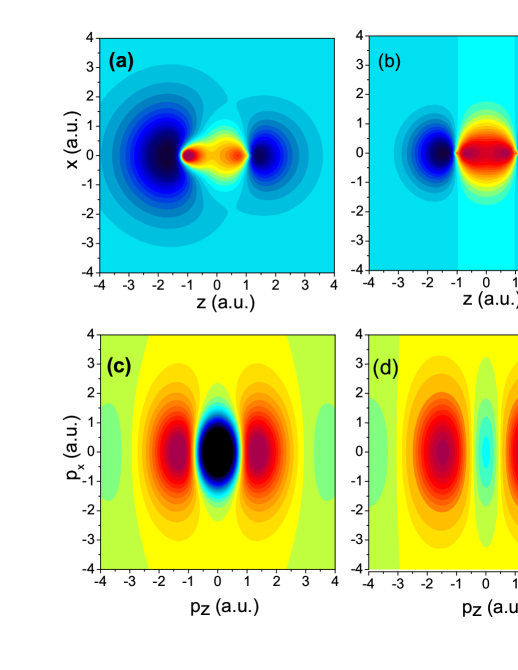
Figure 1: Highest occupied molecular orbitals for CO [panels (a) and (c)] and $\mathrm{N}_{2}$ [panels (b) and (b)], in the position and momentum space (upper and lower panels, respectively).

II.4 Dipole matrix elements

In this section, we will provide explicit expressions for the dipole matrix elements, depending on whether the dipole operator is given in its length or velocity form. We will restrict ourselves to the first-order corrections to the single-active-electron prefactor, as they are expected to be dominant.

II.4.1 Single-active electron approximation

We will commence with the single-active-electron dipole prefactor (7), which is employed in the standard strong-field approximation. In the length form, this prefactor reads

$$a_{\mathrm{l}}^{(0)}(\mathbf{k})=-i\partial_{\mathbf{k}}\psi_{j}(\mathbf{k}),$$ (24)

where $\psi_{j}(\mathbf{k})$ is given by Eq. (II.3). If explicitly written in terms of the wavefunctions centered at the left and right ions,

$$a_{\mathrm{l}}^{(0)}(\mathbf{k}) = i\sum_{\alpha}c_{\alpha,j}^{(L)}\exp[i\mathbf{k\cdot}\frac{\mathbf{R}}{2}]\partial_{\mathbf{k}}\Phi_{\alpha,j}^{(L)}(\mathbf{k})$$ (25)

$$+(-1)^{l_{\alpha}-m_{\alpha}+\lambda_{\alpha}}c_{\alpha,j}^{(R)}\exp[-i\mathbf{k}\cdot\frac{\mathbf{R}}{2}]\partial_{\mathbf{k}}\Phi_{\alpha,j}^{(R)}(\mathbf{k})$$

$$+\frac{\mathbf{R}}{2}\phi_{j}(\mathbf{k}),$$

with

$$\phi_{j}(\mathbf{k}) = \sum_{\alpha}\exp[i\mathbf{k\cdot}\frac{\mathbf{R}}{2}]c_{\alpha,j}^{(L)}\Phi_{\alpha,j}^{(L)}(\mathbf{k})$$

$$-(-1)^{l_{\alpha}-m_{\alpha}+\lambda_{\alpha}}c_{\alpha,j}^{(R)}\exp[-i\mathbf{k\cdot}\frac{\mathbf{R}}{2}]\Phi_{\alpha,j}^{(R)}(\mathbf{k}).$$

The first two terms in Eq. (25)  are mainly oscillating, and give the two-center interference maxima and minima. The third term in Eq. (25) increases with the internuclear distance, and has the main effect of blurring such patterns. In fact, the existence of such term has caused considerable debate and has been attributed to the lack of orthogonality between the continuum and the bound-state wavefunctions in the SFA dressedSFA . Similar terms are also present in the first-order corrections, to be discussed later.

In the velocity form, the single-electron dipole matrix element reads

$$a_{\mathrm{v}}^{(0)} = \sum_{\alpha}c_{\alpha,j}^{(L)}\mathbf{k}\exp[i\mathbf{k\cdot}\frac{\mathbf{R}}{2}]\Phi_{\alpha,j}^{(L)}(\mathbf{k})$$

$$+(-1)^{l_{\alpha}-m_{\alpha}+\lambda_{\alpha}}c_{\alpha,j}^{(R)}\mathbf{k}\exp[-i\mathbf{k\cdot}\frac{\mathbf{R}}{2}]\Phi_{\alpha,j}^{(R)}(\mathbf{k}).$$

In contrast to the length-form scenario, there is no term linearly growing with the internuclear separation. Indeed, previous studies for simplified models for homonuclear molecules indicate that this is the preferred form of the dipole operator, in order to obtain the correct interference patterns JMOCL2007 .

II.4.2 Corrections $a_{\eta}^{(1)}(\mathbf{k})$

We will now write down the explicit forms of Eq. (8) for molecular orbitals in the LCAO approximation. According to Ref. Santra , this term is responsible for the dominant corrections to the single-electron prefactor, and depends on the momentum space wavefunction (II.3), and on the matrix element (10). The former is independent on the form of the dipole operator, while the latter is explicitly given by the sum

$$\mathbf{d}_{\nu\mu}=\sum\limits_{\alpha,l_{\alpha}}\sum\limits_{\beta,l_{\beta}}\sum_{\xi^{\prime},\xi}\Xi_{\xi^{\prime},\xi}(l_{\alpha},l_{\beta})\mathcal{I}_{\xi^{\prime},\xi}^{\alpha,\beta},$$ (28)

where

$$\mathcal{I}_{\xi^{\prime},\xi}^{\alpha,\beta} = \int d^{3}r\left[c_{\alpha,\nu}^{(\xi^{\prime})}\right]^{\ast}c_{\beta,\mu}^{(\xi)}\Phi_{\alpha,\nu}^{\ast(\xi^{\prime})}(\mathbf{r}+(-1)^{a}\mathbf{R}/2)$$ (29)

$$\times d(\mathbf{r})\Phi_{\beta,\mu}^{(\xi)}(\mathbf{r}+(-1)^{b}\mathbf{R}/2).$$

In Eq. (28) and (29), the indices $\xi^{\prime},\xi$ are related to the right or left ions, the exponents $a,b$ are 1 and 0 for $\xi^{\prime},\xi=R$ and $\xi^{\prime},\xi=L,$ respectively, and $d(\mathbf{r})$ denotes the dipole operator in the position representation. In its length and velocity forms, $d^{(l)}(\mathbf{r})=\mathbf{r}$ and $d^{(v)}(\mathbf{r})=i\nabla_{\mathbf{r}}$.The coefficients $\Xi_{\xi^{\prime},\xi}(l_{\alpha},l_{\beta})$ are such that $\Xi_{L,L}(l_{\alpha},l_{\beta})=1,\Xi_{L,R}(l_{\alpha},l_{\beta})=(-1)^{l_{\beta}+\lambda_{\beta}},\Xi_{R,L}(l_{\alpha},l_{\beta})=(-1)^{l_{\alpha}+\lambda_{\alpha}}$ and $\Xi_{R,R}(l_{\alpha},l_{\beta})=(-1)^{l_{\beta}+\lambda_{\beta}+l_{\alpha}+\lambda\alpha}.$

In Eq. (29), one may recognize two types of contributions. The direct integrals

$$\mathcal{I}_{\xi,\xi}^{\alpha,\beta}=\int d^{3}r\left[c_{\alpha,\nu}^{(\xi)}\right]^{\ast}c_{\beta,\mu}^{(\xi)}\Phi_{\alpha,\nu}^{\ast(\xi)}(\mathbf{r}\pm\mathbf{R}/2)d(\mathbf{r})\Phi_{\beta,\mu}^{(\xi)}(\mathbf{r}\pm\mathbf{R}/2),$$ (30)

which contains one-electron wavefunctions centered at the same ion, and the so-called “overlap” integrals

$$\mathcal{I}_{\xi^{\prime},\xi}^{\alpha,\beta}=\int d^{3}r\left[c_{\alpha,\nu}^{(\xi^{\prime})}\right]^{\ast}c_{\beta,\mu}^{(\xi)}\Phi_{\alpha,\nu}^{\ast(\xi^{\prime})}(\mathbf{r}\pm\mathbf{R}/2)d(\mathbf{r})\Phi_{\beta,\mu}^{(\xi)}(\mathbf{r}\mp\mathbf{R}/2),$$ (31)

for $\xi^{\prime}\neq\xi,$ with one-electron wavefunctions localized at different ions. For the moment ignoring the overlap integrals,

$$\mathbf{d}_{\nu\mu} = \sum\limits_{\alpha,l_{\alpha}}\sum\limits_{\beta,l_{\beta}}\left[c_{\alpha,\nu}^{(L)}\right]^{\ast}c_{\beta,\mu}^{(L)}\mathcal{I}_{L,L}^{\alpha,\beta}$$

$$+(-1)^{l_{\beta}+\lambda_{\beta}+l_{\alpha}+\lambda_{\alpha}}\left[c_{\alpha,\nu}^{(R)}\right]^{\ast}c_{\beta,\mu}^{(R)}\mathcal{I}_{R,R}^{\alpha,\beta}.$$

The explicit expressions for the overlap integrals are provided in Appendix 1.

We will commence by providing expressions for (28) using the velocity form. For that purpose, one must solve the integrals (29). Depending on whether the dipole operator couples only $\sigma$ or $\pi$ orbitals, or a $\sigma$ orbital with a $\pi$ orbital, these integrals will be different. If only $\sigma$ orbitals are involved,

$$\mathcal{I}_{\xi,\xi}^{\alpha,\beta}(\sigma,\sigma) = \sum_{j,j^{\prime}}\frac{\pi b_{j,\nu}^{(\xi)}b_{j^{\prime},\mu}^{(\xi)}}{(\zeta_{j,\nu}^{(\xi)}+\zeta_{j^{\prime},\mu}^{(\xi)})}$$

$$\times\left\{l_{\beta}\mathcal{F}(l_{\beta}+l_{\alpha}-1)-2\zeta_{j^{\prime},\mu}^{(\xi)}\mathcal{F}(l_{\beta}+l_{\alpha}+1)\right\},$$

with $\xi=R$ or $L,$ and

$$\mathcal{F}(l)=\frac{1}{2}\left[1+(-1)^{l}\right](\zeta_{j,\nu}^{(\xi)}+\zeta_{j^{\prime},\mu}^{(\xi^{\prime})})^{-1/2-l/2}\Gamma\left[\frac{1+l}{2}\right].$$ (34)

The same expression is encountered if only $\pi_{x}$ or $\pi_{y}$ are coupled, i.e., $\mathcal{I}_{\xi,\xi}^{\alpha,\beta}(\sigma,\sigma)=\mathcal{I}_{\xi,\xi}^{\alpha,\beta}(\pi_{x},\pi_{x})=\mathcal{I}_{\xi,\xi}^{\alpha,\beta}(\pi_{y},\pi_{y}).$ The above-stated expression is only non-vanishing if $l_{\beta}+l_{\alpha}+1$ is even. In our framework, this implies that only $s$ and $p$ states are mixed.  If, on the other hand, a $\sigma$ orbital is coupled to a $\pi_{x}$ or a $\pi_{y}$ orbital, this integral reads

$$\mathcal{I}_{\xi,\xi}^{\alpha,\beta}(\sigma,\pi_{\chi}) = \sum_{j,j^{\prime}}\frac{\sqrt{\pi}b_{j,\nu}^{(\xi)}b_{j^{\prime},\mu}^{(\xi)}}{\left(\zeta_{j,\nu}^{(\xi)}+\zeta_{j^{\prime},\mu}^{(\xi)}\right)^{1/2}}$$ (35)

$$\times(\mathcal{B}(l_{\alpha},l_{\beta})-2\zeta_{j^{\prime},\mu}^{(\xi)}\mathcal{A}(l_{\alpha}+1,l_{\beta})),$$

with $\chi=x,y.$ Thereby,

$$\mathcal{A}(l_{\alpha},l_{\beta})=\mathcal{F}(l_{\alpha})\mathcal{F}(l_{\beta}),$$ (36)

$$\mathcal{B}(l_{\alpha},l_{\beta})=\mathcal{F}(l_{\alpha})\left\{l_{\beta}\mathcal{F}(l_{\beta}-1)-2\zeta_{j^{\prime},\mu}^{(\xi)}\mathcal{F}(l_{\beta}+1)\right\},$$ (37)

and $\mathcal{F}(l_{\beta})$ is defined according to Eq. (34). Eq. (35) also holds for the dipole matric elements coupling the $\pi_{x}$ and $\pi_{y}$ orbitals, i..e, $\mathcal{I}_{\xi,\xi}^{\alpha,\beta}(\sigma,\pi_{\chi})=\mathcal{I}_{\xi,\xi}^{\alpha,\beta}(\pi_{x},\pi_{y})=\mathcal{I}_{\xi,\xi}^{\alpha,\beta}(\pi_{y},\pi_{x}).$ From Eqs. (36) and (37) we see that $\mathcal{A}(l_{\alpha}+1,l_{\beta})\neq 0$ if $l_{\alpha}=0$ and $l_{\beta}=1,$ and that $\mathcal{B}(l_{\alpha},l_{\beta})\neq 0$   if $l_{\alpha}=1$ and $l_{\beta}=0.$ Hence, once more, only $s$ and $p$ states are coupled.

All these contributions are then included in the corrections (8). In the specific case of a homonuclear molecule, an inspection of Eqs. (II.4.2)-(37) shows that only orbitals of different parities are coupled. In fact, if $c_{\alpha,\nu}^{(L)}=c_{\alpha,\nu}^{(R)}$ and $c_{\beta,\mu}^{(L)}=c_{\beta,\mu}^{(R)}$, Eq. (II.4.2) is only nonvanishing if $l_{\beta}+\lambda_{\beta}+l_{\alpha}+\lambda_{\alpha}$ is even. Since, as discussed above, $\mathcal{I}_{\xi,\xi}^{\alpha,\beta}$ are only nonvanishing if $l_{\alpha}$ and $l_{\beta}$ have values corresponding to different parities, this must also hold for $\lambda_{\beta}$ and $\lambda_{\alpha}$. In contrast, for heteronuclear molecules, these coefficients are different and in principle all terms contribute.

We will now state the length-form dipole matrix element. We will mainly consider the integrals $\mathcal{I}_{\xi,\xi}^{\alpha,\beta}.$ If only $\sigma$ orbitals are coupled, these integrals read

$$\mathcal{I}_{\xi,\xi}^{\alpha,\beta}(\sigma,\sigma) = \sum_{j,j^{\prime}}\frac{\pi b_{j,\nu}^{(\xi)}b_{j^{\prime},\mu}^{(\xi)}}{(\zeta_{j,\nu}^{(\xi)}+\zeta_{j^{\prime},\mu}^{(\xi)})}$$

$$\times \left[\mathcal{F}(l_{\alpha}+l_{\beta}+1)\mp\frac{R}{2}\mathcal{F}(l_{\alpha}+l_{\beta})\right],$$

The same expression holds for transitions involving only the $\pi_{x}$ or the $\pi_{y}$ orbitals, i.e., $\mathcal{I}_{\xi,\xi}^{\alpha,\beta}(\sigma,\sigma)=\mathcal{I}_{\xi,\xi}^{\alpha,\beta}(\pi_{x},\pi_{x})=\mathcal{I}_{\xi,\xi}^{\alpha,\beta}(\pi_{y},\pi_{y})$.

If the dipole operator couples $\sigma$ with $\pi$ orbitals, such integrals are given by

$$\mathcal{I}_{\xi,\xi}^{\alpha,\beta}(\sigma,\pi_{\chi}) = \sum_{j,j^{\prime}}\frac{\sqrt{\pi}b_{j,\nu}^{(\xi)}b_{j^{\prime},\mu}^{(\xi)}}{(\zeta_{j,\nu}^{(\xi)}+\zeta_{j^{\prime},\mu}^{(\xi)})^{1/2}}$$

$$\times \left[\mathcal{A}(l_{\alpha}+1,l_{\beta})+\mathcal{A}(l_{\alpha},l_{\beta}+1)\mp\frac{R}{2}\mathcal{A}(l_{\alpha},l_{\beta})\right],$$

with $\chi=x,y.$ Eq. (II.4.2) also holds for couplings between different $\pi$ orbitals, i.e., $\mathcal{I}_{\xi,\xi}^{\alpha,\beta}(\sigma,\pi_{\chi})=\mathcal{I}_{\xi,\xi}^{\alpha,\beta}(\pi_{y},\pi_{x})=\mathcal{I}_{\xi,\xi}^{\alpha,\beta}(\pi_{x},\pi_{y}).$

In the above-stated expressions, one may identify two distinct behaviors. The terms $\mathcal{F}(l_{\alpha}+l_{\beta}+1),$ $\mathcal{A}(l_{\alpha}+1,l_{\beta})$ and $\mathcal{A}(l_{\alpha},l_{\beta}+1)$ are non-vanishing only if $l_{\alpha}$ and $l_{\beta}$ have values corresponding to different parities, i.e., in our framework, it couples $s$ and $p$ states. The terms $\mathcal{F}(l_{\alpha}+l_{\beta})$ and $\mathcal{A}(l_{\alpha},l_{\beta}),$ on the other hand, couple states of the same parity (either $s$ or $p$). For homonuclear molecules, these terms will vanish, as the dipole operator will only couple states of different parities, i.e., $l_{\beta}+l_{\alpha}+1$ must be even in Eq. (II.4.2). For heteronuclear molecules, in contrast, they may in principle be present as the coefficients at each center of the molecule are different.

II.5 Inconsistencies in the dipole matrix elements

We will now discuss some of the subtleties that arise in the evaluation of our multielectron corrections. Firstly, the overlap integrals, in Eq. (31) are often presumed to be very small in comparison to their direct counterpart, but this is not always the case. This can be seen by using the Gaussian theorem,

$$e^{-\zeta_{\alpha}(r-\mathbf{R}/2)^{2}}e^{-\zeta_{\beta}(r+\mathbf{R}/2)^{2}}=Ke^{-\rho(r-\mathbf{R}_{p})^{2}}$$ (40)

where

$$\rho=\zeta_{\alpha}+\zeta_{\beta},$$ (41)

$$K=e^{-\frac{\zeta_{\alpha}\zeta_{\beta}}{\zeta_{\alpha}+\zeta_{\beta}}|\mathbf{R}|^{2}},$$ (42)

and

$$\mathbf{R}_{p}=\frac{\mathbf{R}(\zeta_{\alpha}-\zeta_{\beta})}{2(\zeta_{\alpha}+\zeta_{\beta})}.$$ (43)

Here $\zeta_{\alpha}$ and $\zeta_{\beta}$ correspond to our exponents in Eq. (17).

At first sight it would appear that these contributions are much smaller than those from the direct integrals (30). This does not hold, however, for exponents that are less than unity, of which there are many for various different atomic orbitals. It is therefore not astute to ignore the overlap integrals in this instance.

In fact, we have verified that in most cases the overlap integrals (31) are comparable to the integrals (30) at the same center. More importantly, we have also found that the velocity form gives zero static dipole moment for heteronuclear molecules when using a Gaussian basis set. This is an unphysical result, which has been verified for the direct integrals by using the properties of Gamma functions to analyze the term in brackets in Eq. (II.4.2). Explicitly, it can be shown that this term is proportional to $[\zeta_{j}l_{\beta}-\zeta_{j}^{\prime}l_{\alpha}/(\zeta_{j}^{\prime}+\zeta_{j})]$. Since only $s$ and $p$ states can be coupled, each pair $(l_{\alpha},l_{\beta})=(0,1)$ and $(l_{\alpha},l_{\beta})=(1,0)$ will lead to symmetric contributions which will cancel out. We have also verified numerically that the overlap integrals are vanishingly small in this case.

Apart from that, inclusion of the overlap integrals gives rise to terms that depend on R, and thus removes the translational invariance from the velocity form. This problem is also encountered in the single-active electron matrix element when using the length form. In contrast to the one-electron length-form scenario, however, these terms will vanish at large internuclear distances due to the Gaussian exponentials (42). (see a discussion in dressedSFA for their counterpart in the single-active electron framework)

In contrast, the length form predicts non-zero static dipole moment in heteronuclear molecules, which makes sense physically. However, for the heteronuclear case the R-dependent terms that arise in the direct integrals couple states of the same parity as seen in Eq. (II.4.2) and Eq. (II.4.2). This should not occur for an odd operator such as the dipole, which is an unphysical result. This is another reason to suggest that these terms should be neglected. In the results that follows, this term will be neglected unless otherwise stated.

III High-order harmonic spectra

Below we compare the harmonic spectra predicted by different forms of the dipole operator. We will place particular emphasis on the comparison between homonuclear and heteronuclear molecules. The former and the latter will be exemplified by $\mathrm{N}_{2}$ and CO, respectively. We will consider the full, three-dimensional dynamics of the problem. For that purpose, one must integrate over the azimuthal coordinate, $\phi_{p}$, such that,

$$S(\Omega)=\int_{0}^{2\pi}|M|^{2}d\phi_{k},$$ (44)

where $\ M$ is the overall transition amplitude. This allows one to consider the degeneracy of the $\pi$ orbitals CarlaBrad . The corrections are incorporated in the ionization and recombination prefactors. The former gives the particular weight for tunneling to take place, and the latter gives the shape of the high-order harmonic spectra and the two-center fringes. The explicit expressions for the dipole matrix elements are provided in Appendix 2.

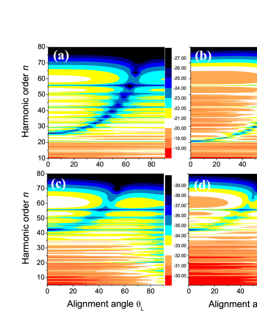
Figure 2: High-order harmonic spectra for $\mathrm{N}_{2}$ subject to a linearly polarized laser field of frequency $\omega=0.057$ a.u. and intensity $I=4\times 10^{14}\mathrm{W/cm}^{2}$, as a function of the alignment angle $\theta_{L}$ between the molecule and the field. In the figure we consider the corrections in both the ionization and the recombination prefactors. Panels (a) and (c) have been computed employing the length form, while panels (b) and (d) have been calculated using the velocity form. The upper panels display the $3\sigma_{g}$ spectrum in which the first-order corrections have been incorporated. In the lower panels, we depict the yield obtained with the first order corrections in the length and the velocity form. The bound-state energy of the HOMO and the equilibrium internuclear distance have been taken from GAMESS-UK. Explicitly, $\epsilon^{(\mathrm{N}_{2})}_{0}=0.63485797$ a.u and $R^{(\mathrm{N}_{2})}=2.068$ a.u. The contour plots have been normalized with regard to the maximum yield in each panel.

We will now start by discussing the high-harmonic spectra of diatomic nitrogen ($\mathrm{N}_{2}$) computed including the single-atom prefactor and the first-order corrections. In Fig. 2, we display such spectra, in the velocity and length form (panels (a) and (b), respectively), together with the corrections alone (panels (c) and (d), respectively). In the length-form prefactor $a_{\sigma}^{(0)}(\mathbf{k})$, we omitted the term growing linearly with the internuclear distance $R$. In the corrections, we included both the direct and the overlap integrals.

In the figure, we notice a clear two-center minimum, which is due to the interference of high-harmonic emission at the two spatially separated centers in the molecule. This minimum varies with the alignment angle $\theta_{L}$ of the molecule with respect to the laser-field polarization. In the upper panels, its energy position is characteristic of the $3\sigma_{g}$ orbital DM2009 ; CarlaBrad . A comparison of panels (a) and (b) shows that the two-center minimum is slightly displaced, depending on the form of the dipole operator. For instance, for vanishing alignment angle, in the velocity form this minimum is near $\Omega=21\omega$, while in the length form it is at a slightly higher energy ($\Omega=25\omega$). This is due to the fact that the $s-p$ mixing, which determines the energy position of this minimum, is different for each case. The velocity form slightly favors the contributions from the $p$ states, compared to the length form. For a discussion of the $s-p$ mixing in a slightly different context, namely of different basis sets, and its influence on the high-order harmonic spectra, see CarlaBrad . Here, however, this bias is introduced by the different forms of the dipole operator.

The remaining panels exhibit the spectra obtained employing the first-order corrections only. Such contributions exhibit a well-defined minimum, whose position is at a quite different energy from that observed in the overall prefactor. We have verified that this pattern can be related to the contributions of the $\sigma_{u}$ orbitals. The contributions of the $\pi_{u}$ orbitals are strongly suppressed in this parameter region due to to the presence of a nodal plane along the internuclear axis.

Quantitatively, the yield in panels (c) and (d) is several orders of magnitude smaller than those in the upper panels. This shows that, in the present framework, it suffices to consider the zeroth order contributions. This behavior occurs both for the length and the velocity form of the dipole operator, and is due to the fact that the corrections are considerably smaller both in the ionization and recombination prefactor. The above-mentioned suppression of ionization for the $\pi$ orbitals also contributes to such results.

The influence of the ionization prefactor can be seen in Fig. 3. Therein, we present spectra computed for a fixed alignment angle assuming $a_{\mathrm{ion}}(\mathbf{k}+\mathbf{A}(t_{0}))$ to be constant and equal to unity. Physically, this implies that any influence of the orbital symmetry on tunneling ionization, such as the presence or absence of nodal planes, has been removed, both for the zeroth-order prefactor and the corrections. For comparison, we are also providing the full spectra, with both the ionization and recombination prefactors.

The figure shows that, while the overall spectra changes relatively little, or may even increase if this prefactor is removed (see orange and black lines in Fig. 3.(a)), the corrections increase in several orders of magnitude. This can be attributed to the following. In the parameter range of interest, the zeroth order ionization prefactor, which is the main influence in the overall spectra, is of the order of unity or even slightly larger for a $3\sigma_{g}$ orbital. This is due to the absence of nodal planes for either parallel or perpendicular alignment in this particular case. In contrast, in the corrections, mainly $\sigma_{u}$ or $\pi_{u}$ orbitals are involved. The former orbitals exhibit nodal planes for alignment angles $\theta_{L}=90^{\circ}$ and the latter for $\theta_{L}=0$. This will cause an overall suppression in tunnel ionization for a wide range of angles, when such orbitals are summed over. Furthermore, the dipole matrix elements $d_{\mu\nu}$ in the spectra are quite small and will also contribute to the above-mentioned suppression.

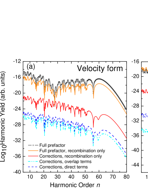
Figure 3: High-order harmonic spectra for $\mathrm{N}_{2}$ in a driving field with the same parameters as in the previous figure, and an alignment angle $\theta_{L}=\pi/4$. The figure shows the overall spectra together with the first-order corrections taking into account only the direct or overlap integrals. We consider both the ionization and recombination prefactors, or the recombination prefactor only (orange and red lines in the figure). Panels (a) and (b) give the velocity and length forms of the dipole operator, respectively.

Another noteworthy feature also presented in Fig. 3 is the influence of the so-called overlap integrals, in which the dipole operator couples wavefunctions at different centers in the molecule, in the multielectron corrections. In general, these integrals are assumed to be very small in comparison with the direct integrals, in which wavefunctions at the same ion are taken. Hence, in many cases the overlap integrals are neglected. We have verified, however, that this depends strongly on the form of the dipole operator. For the velocity-form dipole, the spectra obtained from the overlap integrals are comparable to those obtained from the direct integrals only [Fig. 3.(a)]. Hence, both contributions must be included. In contrast, if the length form is considered, the contributions from the overlap integrals are considerably smaller than their direct-integral counterparts [Fig. 3.(b)]. Therefore, the former may be neglected.

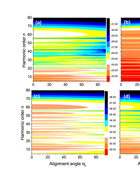
Figure 4: High-order harmonic spectra for CO in a driving field with the same parameters as in the previous figure, as a function of the alignment angle. Panels (a) and (c) exhibit the full spectra and the corrections in the length form, while panels (b) and (d) give their counterparts in the velocity form. In the length form, the linearly growing terms with regard to the internuclear distance have been neglected.

Next, we will discuss the spectra encountered for CO. The overall spectra are depicted in Fig. 4, together with the first-order corrections (upper and lower panels, respectively). As an overall feature, the spectra exhibit no perceivable two-center interference minimum, as CO is a heteronuclear molecule. This means that, upon recombination, there will be more high-order harmonic emission from a specific spatial region, where the orbital with which the electron recombines, i.e., the HOMO, is more localized. This occurs both for the velocity and length forms (Figs. 4.(a) and (b), respectively).

One notices, however, that the decrease in the overall yield as the molecular alignment angle approaches $\theta_{L}=90^{\circ}$ remains, due to the fact that the HOMO is a $\sigma$ orbital, and thus highly localized along the internuclear axis. As the laser-field polarization direction moves away from this axis, recombination, and hence high-order harmonic emission becomes less and less probable. Due, however, to the heteronuclear nature of this molecule, this suppression occurs at a different angle compared to $\mathrm{N}_{2}$.

Once more, we find that the contributions of the first-order multielectron corrections to the spectra are several orders of magnitude smaller than the zeroth-order terms. These contributions are depicted in Fig. 4.(c) and (d), for the length and velocity form, respectively. For such corrections, the interference minimum due to high-harmonic emission at different centers has been washed out. This minimum was very clear for $\mathrm{N}_{2}$ (see Figs. 2.(c) and (d) for comparison). There is, however, a very pronounced minimum near $\theta_{L}=50^{\circ}$ for the velocity-form corrections, which is independent of the harmonic frequency (see Fig. 4.(d)). This minimum is due to the geometry of the three lower-lying $\sigma$ orbitals, which influence the corrections. This suggests that the imprints on the high-order harmonic spectra due to purely geometric features, such as nodal planes or minima in the orbitals, are more robust than those related to quantum interference between harmonics emitted as spatially separated centers. The length-form corrections, in contrast, do not exhibit any such feature. In fact, we have verified that they are dominated by the static dipole moment, which behaves in the same way as the HOMO.

Below, in Fig. 5, we perform a more detailed analysis of the above-mentioned issue. For that purpose, we consider the contributions of individual orbitals to the corrections, and their influence on the harmonic spectra, for fixed harmonic order. We consider a mid-plateau harmonic, namely $\Omega=45\omega$. These results are displayed for both $\mathrm{N}_{2}$ and CO, as functions of the alignment angle (upper and lower panels in the figure, respectively). As an overall feature, we observe that, for a homonuclear molecule, all contributions are symmetric upon $\theta\rightarrow\theta+\pi$ (see panels(a) and (b)). Physically, this is expected, as such molecules exhibit inversion symmetry and a rotation of $\pi$ should not alter the physics of the problem. Clearly, this no longer holds for a heteronuclear molecule. In this latter case, however, the contribution of $S_{n}(\theta_{L})$ to the yield is the mirror image of $S_{n}(\theta_{L}+\pi)$. This is clear, as in this case the right and the left ions are reversed.

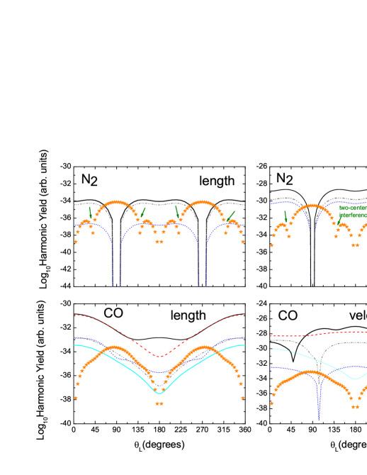
Figure 5: Contributions of individual orbitals to the first-order corrections in the $45_{th}$ harmonic of a field with the same parameters as in the previous figures, as functions of the alignment angle $\theta_{L}$ of the molecule relative to the laser-field polarization. The thick black lines in the panel give the overall contributions of all $\sigma$ orbitals and the orange stars the contributions of the $\pi$ orbitals, respectively. Panels (a) and (b) refer to $\mathrm{N}_{2}$, and panels (c) and (d) correspond to CO, respectively. The left and right panels display the results using the length and velocity form of the dipole operator, respectively. The minima due to the two-center interference are indicated by green arrows in the figure.

The individual contributions provide useful information about the geometry of the orbitals involved in the corrections. This can be seen in all cases, regardless of whether the molecule is heteronuclear or homonuclear. For instance, the contributions from the $\pi$ orbitals, shown as the orange symbols in the figure, decay very abruptly for $\theta_{L}=n\pi$. This is due to the fact that such orbitals exhibit nodal planes in the case of $\mathrm{N}_{2}$ and a feature similar to nodal planes in the case of CO. The main difference between the homonuclear and the heteronuclear case is the two-center interference minimum, which is absent in the heteronuclear case. Furthermore, the shapes of such distributions do not change with the form of the dipole operator. Any changes are mostly quantitative (for a comparison, see panels (a) and (b) for $\mathrm{N}_{2}$ and panels (c) and (d) for CO).

The contributions from the $\sigma$ orbitals, on the other hand, can behave in very different ways depending on whether the velocity or the length form is taken, in the heteronuclear case, such as CO. For $\mathrm{N}_{2}$, in contrast, different forms of the dipole operator will mainly lead to a different weighting of the contributions from individual orbitals to the overall corrections. For instance, in the length-form case, the contributions of the $2\sigma_{u}$ orbital are prevalent, while if the velocity form is taken, the contributions from both $\sigma_{u}$ orbitals are comparable. Another interesting feature is that both forms lead to a sharp harmonic suppression near $\theta_{L}=(2n+1)\pi/2$. This is due to the fact that the nodal planes of the $1\sigma_{u}$ and $2\sigma_{u}$ orbitals are parallel to the laser-field polarization for such angles.

In CO, however, we notice two interesting features. Firstly, the nodes disappear if the length form is taken. This is partly due to the static dipole moment, which is only present in the length form and leads to corrections which behave like the HOMO. This implies that the overall dipole will decrease for $\theta_{L}=\pi$ as shown in the figure. In contrast, in the velocity form, as this term is absent, there are minima near $\theta_{L}=\pi/4$. These minima come from the geometry of $2\sigma$ and $4\sigma$, which are the heteronuclear counterparts of $1\sigma_{u}$ and $2\sigma_{u}$, leading to a strong suppression in the yield close to $\theta_{L}=(2n+1)\pi/2$. They are, however, slightly shifted from these values due to the heteronuclear character of the molecule. The remaining $\sigma$ orbitals shift these minima even further, to $\theta_{L}\simeq\pi/4$.

IV Conclusions

In conclusion, our results show that an adequate choice of the dipole operator in order to model high-order harmonic generation is still an open question. In the single-active-electron approximation, enough evidence has been provided in JMOCL2007 that the velocity form yields the best agreement with the double-slit physical picture. If one goes beyond this approximation, however, the velocity form leads to a vanishing static dipole moment for heteronuclear molecules. This may be a particularity of the basis set involved.

Another issue in the velocity form are the so-called overlap integrals, in which the dipole operator couples wavefunctions localized at different ions in the molecule. Throughout the literature, it has been argued that such integrals are small and may be neglected without loss of information. Our results, however, indicate that, depending on the basis set used, their outcome may be comparable to that of the direct integrals, in which wavefunctions at the same ion are coupled. As the internuclear distance increases, however, the overlap integrals become vanishing small.

In contrast, the length-form of the dipole operator leads to a non-vanishing static dipole moment for a heteronuclear molecule, and very small overlap integrals, in comparison to their direct counterparts. The main problem, however, is that such a formulation leads to terms in the dipole-matrix elements with increase indefinitely with the internuclear separation. They also couple states with the same parity, which is unphysical for an odd operator such as the dipole. Such terms have been also found in the single-active electron context JMOCL2007 . Hence, it seems that the velocity form still gives better results.

Furthermore, suppression of the harmonic spectra caused by the presence of nodes in the orbitals is far more robust than the maxima and minima coming from two-center interference. Interestingly, for heteronuclear molecules, despite interference minima being washed out, the high-harmonic suppression caused by the geometry of the orbitals is still present in the spectra. However, compared to their homonuclear counterpart, this suppression occurs at different alignment angles.

Finally, in order to incorporate multielectron effects in SFA-like models in an appropriate way, one must consider the dynamics of the target. Concrete examples are excitation, relaxation, electron orbits starting or finishing at different molecular orbitals, or the motion of the bound electrons. This paper has shown that, if multielectron effects are considered statically by employing many-body perturbation theory around the single-electron strong-field approximation, they lead to corrections which are several orders of magnitude smaller than the zeroth-order spectrum. This holds for both homonuclear and heteronuclear molecules. In fact, recent results in which excitation or relaxation have been incorporated numerically exhibited larger corrections Smirnova ; Patchkovskii .

Acknowledgements: We profited from several discussions with H. J. J. van Dam, P. J. Durham, P. Sherwood and in particular J. Tennyson. This work has been funded by the UK EPSRC and by the Daresbury Laboratory.

V Appendix 1: Overlap integrals for dipole matrix elements

In this appendix, we are providing the generalized expressions for the overlap integrals (31) considering the dipole operator in its velocity and length forms.

V.1 Velocity form

We will commence by the velocity-form expressions. If only $\sigma$ orbitals are coupled,one may show that

$$\mathcal{I}_{\xi,\xi^{\prime}}^{\alpha,\beta}(\sigma,\sigma) = \sum_{j,j^{\prime}}\frac{\pi b_{j,\nu}^{(\xi)}b_{j^{\prime},\mu}^{(\xi^{\prime})}}{\zeta_{j,\nu}^{(\xi)}+\zeta_{j^{\prime},\mu}^{(\xi^{\prime})}}e^{-\frac{\zeta_{j,\nu}^{(\xi)}\zeta_{j^{\prime},\mu}^{(\xi^{\prime})}}{\zeta_{j,\nu}^{(\xi)}+\zeta_{j^{\prime},\mu}^{(\xi^{\prime})}}R^{2}}$$

$$\times[l_{\beta}\mathcal{J}(l_{\alpha},l_{\beta}-1)-2\zeta_{j^{\prime},\mu}^{(\xi^{\prime})}\mathcal{J}(l_{\alpha},l_{\beta}+1)],$$

where

$$\mathcal{J}(l_{\alpha},l_{\beta}) = \int_{-\infty}^{\infty}\left[u\pm\frac{\rho_{j^{\prime},j,\mu,\nu}^{(\xi)}}{2}R\right]^{l_{\beta}}\left[u\mp\frac{\rho_{j,j^{\prime},\nu,\mu}^{(\xi^{\prime})}}{2}R\right]^{l\alpha}$$ (46)

$$\times\exp[-(\zeta_{j,\nu}^{(\xi)}+\zeta_{j^{\prime},\mu}^{(\xi^{\prime})})u^{2}]du,$$

with

$$\rho_{j,j^{\prime},\nu,\mu}^{(\xi)}=\frac{-2\zeta_{j^{\prime},\mu}^{(\xi)}}{\zeta_{j,\nu}^{(\xi)}+\zeta_{j^{\prime},\mu}^{(\xi)}},$$ (47)

$$u=z\pm\frac{\zeta_{j,\nu}^{(\xi)}-\zeta_{j^{\prime},\mu}^{(\xi^{\prime})}}{2(\zeta_{j,\nu}^{(\xi)}+\zeta_{j^{\prime},\mu}^{(\xi^{\prime})})}R$$ (48)

and $\mathcal{J}(l_{\alpha},l_{\beta}-1)=0$ for $l_{\beta}=0.$

If, on the other hand, we consider a transition from a $\sigma$ to a $\pi_{x}$ or $\pi_{y}$ orbital,

$$\mathcal{I}_{\xi,\xi^{\prime}}^{\alpha,\beta}(\sigma,\pi_{\chi}) = \sum_{j,j^{\prime}}\frac{\sqrt{\pi}b_{j,\nu}^{(\xi)}b_{j^{\prime},\mu}^{(\xi^{\prime})}}{\left(\zeta_{j,\nu}^{(\xi)}+\zeta_{j^{\prime},\mu}^{(\xi^{\prime})}\right)^{1/2}}e^{-\frac{\zeta_{j,\nu}^{(\xi)}\zeta_{j^{\prime},\mu}^{(\xi^{\prime})}}{\zeta_{j,\nu}^{(\xi)}+\zeta_{j^{\prime},\mu}^{(\xi^{\prime})}}R^{2}}$$ (49)

$$\times\left[l_{\beta}\mathcal{C}(l_{\beta}-1,l_{\alpha},0)-2\zeta_{j^{\prime},\mu}^{(\xi^{\prime})}\left[\mathcal{C}(l_{\beta},l_{\alpha},1)+\mathcal{C}(l_{\beta}+1,l_{\alpha},0)\right]\right],$$

where $\mathcal{C}(l_{\alpha},l_{\beta},l_{\gamma})=\mathcal{F}(l_{\alpha})\mathcal{J}(l_{\beta},l_{\gamma}).$ The function $\mathcal{F}(l_{\alpha})$ is defined in Eq. (34). If only $\pi_{x}$ or $\pi_{y}$ orbitals are coupled, the overlap integrals read

$$\mathcal{I}_{\xi,\xi^{\prime}}^{\alpha,\beta}(\pi_{\chi},\pi_{\chi}) = \sum_{j,j^{\prime}}\frac{\sqrt{\pi}b_{j,\nu}^{(\xi)}b_{j^{\prime},\mu}^{(\xi^{\prime})}}{\left(\zeta_{j,\nu}^{(\xi)}+\zeta_{j^{\prime},\mu}^{(\xi^{\prime})}\right)^{1/2}}e^{-\frac{\zeta_{j,\nu}^{(\xi)}\zeta_{j^{\prime},\mu}^{(\xi^{\prime})}}{\zeta_{j,\nu}^{(\xi)}+\zeta_{j^{\prime},\mu}^{(\xi^{\prime})}}R^{2}}$$ (50)

$$\times \left[l_{\beta}\mathcal{C}(l_{\beta}+l_{\alpha}-1,0,0)-2\zeta_{j^{\prime},\mu}^{(\xi^{\prime})}\left[\mathcal{C}(l_{\beta}+l_{\alpha},0,1)+\mathcal{C}(l_{\beta}+l_{\alpha}+1,0,0)\right]\right],$$

with $\chi=x$ or $y.$ Finally, if we consider the overlap integral coupling different $\pi$ orbitals, we will find

$$\mathcal{I}_{\xi,\xi^{\prime}}^{\alpha,\beta}(\pi_{\lambda},\pi_{\chi}) = \sum_{j,j^{\prime}}\frac{\sqrt{\pi}b_{j,\nu}^{(\xi)}b_{j^{\prime},\mu}^{(\xi^{\prime})}}{\left(\zeta_{j,\nu}^{(\xi)}+\zeta_{j^{\prime},\mu}^{(\xi^{\prime})}\right)^{1/2}}e^{-\frac{\zeta_{j,\nu}^{(\xi)}\zeta_{j^{\prime},\mu}^{(\xi^{\prime})}}{\zeta_{j,\nu}^{(\xi)}+\zeta_{j^{\prime},\mu}^{(\xi^{\prime})}}R^{2}}$$

$$\times\{-2\zeta_{j^{\prime},\mu}^{(\xi^{\prime})}\mathcal{G}(l_{\alpha},l_{\beta})+l_{\beta}\mathcal{H}(l_{\alpha},l_{\beta}-1,0,0)\}.$$

with

$$\mathcal{G}(l_{\alpha},l_{\beta}) = \mathcal{H}(l_{\alpha},l_{\beta},0,1)$$

$$+\mathcal{H}(l_{\alpha}+1,l_{\beta},0,0)+\mathcal{H}(l_{\alpha},l_{\beta}+1,0,0)$$

and $\mathcal{H}(l_{\alpha},l_{\beta},l_{\gamma},l_{\delta})=\mathcal{A}(l_{\alpha},l_{\beta})\mathcal{J}(l_{\gamma},l_{\delta}).$ In Eq. (V.1), $\lambda\neq\chi.$ The function $\mathcal{A}(l_{\alpha},l_{\beta})$ is defined in Eq. (36).

V.2 Length form

For the length form of the dipole operator, if only transitions involving $\sigma$ orbitals are considered, we find that

$$\mathcal{I}_{\xi,\xi^{\prime}}^{\alpha,\beta}(\sigma,\sigma)=\sum_{j,j^{\prime}}\frac{\pi b_{j,\nu}^{(\xi)}b_{j^{\prime},\mu}^{(\xi^{\prime})}}{\zeta_{j,\nu}^{(\xi)}+\zeta_{j^{\prime},\mu}^{(\xi^{\prime})}}e^{-\frac{\zeta_{j,\nu}^{(\xi)}\zeta_{j^{\prime},\mu}^{(\xi^{\prime})}}{\zeta_{j,\nu}^{(\xi)}+\zeta_{j^{\prime},\mu}^{(\xi^{\prime})}}R^{2}}\mathcal{K}(l_{\alpha},l_{\beta}),$$ (53)

where

$$\mathcal{K}(l_{\alpha},l_{\beta}) =\int_{-\infty}^{\infty}\left[u\pm\frac{\rho_{j^{\prime},j,\mu,\nu}^{(\xi)}}{2}R\right]^{l_{\beta}}\left[u\mp\frac{\rho_{j,j^{\prime},\nu,\mu}^{(\xi^{\prime})}}{2}R\right]^{l\alpha}$$

$$\times\left[u\mp\frac{\zeta_{j,\nu}^{(\xi)}-\zeta_{j^{\prime},\mu}^{(\xi^{\prime})}}{2(\zeta_{j,\nu}^{(\xi)}+\zeta_{j^{\prime},\mu}^{(\xi^{\prime})})}R\right]\exp[-(\zeta_{j,\nu}^{(\xi)}+\zeta_{j^{\prime},\mu}^{(\xi^{\prime})})u^{2}]du.$$

For transitions from a $\sigma$ to a $\pi_{x}$ or $\pi_{y}$ orbital, the overlap integral reads

$$\mathcal{I}_{\xi,\xi^{\prime}}^{\alpha,\beta}(\sigma,\pi_{\chi}) = \sum_{j,j^{\prime}}\frac{\sqrt{\pi}b_{j,\nu}^{(\xi)}b_{j^{\prime},\mu}^{(\xi^{\prime})}}{\left(\zeta_{j,\nu}^{(\xi)}+\zeta_{j^{\prime},\mu}^{(\xi^{\prime})}\right)^{1/2}}e^{-\frac{\zeta_{j,\nu}^{(\xi)}\zeta_{j^{\prime},\mu}^{(\xi^{\prime})}}{\zeta_{j,\nu}^{(\xi)}+\zeta_{j^{\prime},\mu}^{(\xi^{\prime})}}R^{2}}$$

$$\times\left\{\mathcal{F}[l_{\alpha}+1]\mathcal{J}(0,l_{\beta})+\mathcal{F}[l_{\alpha}]\mathcal{K}(0,l_{\beta})\right\},$$

with $\chi=x$ or $y.$

Finally, if only $\pi$ orbitals are involved, one may distinguish two types of overlap integrals. Either the dipole matrix element couples the same initial and final orbital, $\pi_{x}$ or $\pi_{y},$or the orbitals $\pi_{\chi}$ and $\pi_{\lambda},$ $\chi\neq\lambda.$ The former case is given by

$$\mathcal{I}_{\xi,\xi^{\prime}}^{\alpha,\beta}(\pi_{\chi},\pi_{\chi}) =\sum_{j,j^{\prime}}\frac{\sqrt{\pi}b_{j,\nu}^{(\xi)}b_{j^{\prime},\mu}^{(\xi^{\prime})}}{\left(\zeta_{j,\nu}^{(\xi)}+\zeta_{j^{\prime},\mu}^{(\xi^{\prime})}\right)^{1/2}}e^{-\frac{\zeta_{j,\nu}^{(\xi)}\zeta_{j^{\prime},\mu}^{(\xi^{\prime})}}{\zeta_{j,\nu}^{(\xi)}+\zeta_{j^{\prime},\mu}^{(\xi^{\prime})}}R^{2}}$$

$$\times\left\{\mathcal{F}[l_{\alpha}+l_{\beta}+1]\mathcal{J}(0,0)+\mathcal{F}[l_{\alpha}+l_{\beta}]\mathcal{K}(0,0)\right\},$$

while the latter reads

$$\mathcal{I}_{\xi,\xi^{\prime}}^{\alpha,\beta}(\pi_{\lambda},\pi_{\chi}) = \sum_{j,j^{\prime}}\frac{\sqrt{\pi}b_{j,\nu}^{(\xi)}b_{j^{\prime},\mu}^{(\xi^{\prime})}}{\left(\zeta_{j,\nu}^{(\xi)}+\zeta_{j^{\prime},\mu}^{(\xi^{\prime})}\right)^{1/2}}e^{-\frac{\zeta_{j,\nu}^{(\xi)}\zeta_{j^{\prime},\mu}^{(\xi^{\prime})}}{\zeta_{j,\nu}^{(\xi)}+\zeta_{j^{\prime},\mu}^{(\xi^{\prime})}}R^{2}}$$

$$\times\left\{\mathcal{E}(l_{\alpha},l_{\beta})\mathcal{J}(0,0)+\mathcal{A}(l_{\alpha},l_{\beta})\mathcal{K}(0,0)\right\},$$

with $\mathcal{E}(l_{\alpha},l_{\beta})=$ $\mathcal{A}(l_{\alpha},l_{\beta}+1)+\mathcal{A}(l_{\alpha}+1,l_{\beta}).$

V.3 Particular integrals $\mathcal{J}$ and $\mathcal{K}$

Specifically for the basis set employed in this work, we find

$$\mathcal{J}(0,0)=\sqrt{\frac{\pi}{\zeta_{j,\nu}^{(\xi)}+\zeta_{j^{\prime},\mu}^{(\xi^{\prime})}}},$$ (58)

$$\mathcal{J}(0,1)=\pm\frac{\sqrt{\pi}\zeta_{j,\nu}^{(\xi)}R}{\left(\zeta_{j,\nu}^{(\xi)}+\zeta_{j^{\prime},\mu}^{(\xi^{\prime})}\right)^{3/2}},$$ (59)

$$\mathcal{J}(1,1)=\frac{\sqrt{\pi}}{2\left(\zeta_{j,\nu}^{(\xi)}+\zeta_{j^{\prime},\mu}^{(\xi^{\prime})}\right)^{3/2}}\left[1-\frac{2\zeta_{j,\nu}^{(\xi)}\zeta_{j^{\prime},\mu}^{(\xi^{\prime})}}{\zeta_{j,\nu}^{(\xi)}+\zeta_{j^{\prime},\mu}^{(\xi^{\prime})}}R^{2}\right],$$ (60)

$$\mathcal{J}(0,2)=\frac{\sqrt{\pi}}{2\left(\zeta_{j,\nu}^{(\xi)}+\zeta_{j^{\prime},\mu}^{(\xi^{\prime})}\right)^{3/2}}\left[1+\frac{2\left(\zeta_{j,\nu}^{(\xi)}\right)^{2}}{\zeta_{j,\nu}^{(\xi)}+\zeta_{j^{\prime},\mu}^{(\xi^{\prime})}}R^{2}\right]$$ (61)

and

$$\mathcal{J}(1,2) = \pm\frac{\sqrt{\pi}}{2\left(\zeta_{j,\nu}^{(\xi)}+\zeta_{j^{\prime},\mu}^{(\xi^{\prime})}\right)^{5/2}}$$

$$\times\left[(\zeta_{j^{\prime},\mu}^{(\xi^{\prime})}-2\zeta_{j,\nu}^{(\xi)})R+\frac{2\zeta_{j^{\prime},\mu}^{(\xi^{\prime})}\left(\zeta_{j,\nu}^{(\xi)}\right)^{2}}{\left(\zeta_{j,\nu}^{(\xi)}+\zeta_{j^{\prime},\mu}^{(\xi^{\prime})}\right)}R^{3}\right].$$

for the integrals $\mathcal{J}(l_{\alpha},l_{\beta}\pm 1)$ and $\mathcal{J}(0,l_{\beta}),$ and

$$\mathcal{K}(0,0)=\mp\sqrt{\frac{\pi}{\zeta_{j,\nu}^{(\xi)}+\zeta_{j^{\prime},\mu}^{(\xi^{\prime})}}}\frac{\zeta_{j,\nu}^{(\xi)}-\zeta_{j^{\prime},\mu}^{(\xi^{\prime})}}{2(\zeta_{j,\nu}^{(\xi)}+\zeta_{j^{\prime},\mu}^{(\xi^{\prime})})}R,$$ (63)

$$\mathcal{K}(0,1)=\frac{\sqrt{\pi}}{2\left(\zeta_{j,\nu}^{(\xi)}+\zeta_{j^{\prime},\mu}^{(\xi^{\prime})}\right)^{3/2}}\left[1+\frac{\zeta_{j,\nu}^{(\xi)}(\zeta_{j,\nu}^{(\xi)}-\zeta_{j^{\prime},\mu}^{(\xi^{\prime})})}{2\left(\zeta_{j,\nu}^{(\xi)}+\zeta_{j^{\prime},\mu}^{(\xi^{\prime})}\right)}R^{2}\right],$$ (64)

$$\mathcal{K}(1,0)=\frac{\sqrt{\pi}}{2\left(\zeta_{j,\nu}^{(\xi)}+\zeta_{j^{\prime},\mu}^{(\xi^{\prime})}\right)^{3/2}}\left[1-\frac{\zeta_{j^{\prime},\mu}^{(\xi^{\prime})}(\zeta_{j,\nu}^{(\xi)}-\zeta_{j^{\prime},\mu}^{(\xi^{\prime})})}{2\left(\zeta_{j,\nu}^{(\xi)}+\zeta_{j^{\prime},\mu}^{(\xi^{\prime})}\right)}R^{2}\right]$$ (65)

and

$$\mathcal{K}(1,1)=\mp\frac{\sqrt{\pi}(\zeta_{j,\nu}^{(\xi)}-\zeta_{j^{\prime},\mu}^{(\xi^{\prime})})}{2\left(\zeta_{j,\nu}^{(\xi)}+\zeta_{j^{\prime},\mu}^{(\xi^{\prime})}\right)^{5/2}}\left[\frac{3R}{2}-\frac{\zeta_{j,\nu}^{(\xi)}\zeta_{j^{\prime},\mu}^{(\xi^{\prime})}}{\zeta_{j,\nu}^{(\xi)}+\zeta_{j^{\prime},\mu}^{(\xi^{\prime})}}R^{3}\right]$$ (66)

for the integrals $\mathcal{K}(l_{\alpha},l_{\beta})$. The above-stated expressions show that the integrals $\mathcal{J}(l_{\alpha},l_{\beta}\pm 1)$ and $\mathcal{K}(l_{\alpha},l_{\beta})$ will lead to a polynomial dependence on $R/(\zeta_{j,\nu}^{(\xi)}+\zeta_{j^{\prime},\mu}^{(\xi^{\prime})})^{1/2+n}$. This dependence will be damped by the gaussian factor in Eq. (V.1), so that the overlap integrals are expected to decrease with the internuclear distance.

VI Appendix 2: Angle-integrated dipole matrix elements

In this appendix, we provide the expressions obtained for the dipole matrix elements, if the azimuthal angular variable is integrated over. Let us start with $\mathrm{N}_{2}$. In this case, the HOMO is a $3\sigma_{g}$ orbital. The orbitals that will contribute to the corrections are $1\pi_{u_{x}}$, $1\pi_{u_{y}}$, $2\sigma_{u}$ and 1$\sigma_{u}$. The remaining, $\sigma_{g}$ orbitals do not contribute to the corrections for symmetry reasons. We will be able then to write for the first-order dipole matrix element,

$$d^{(1)}(\mathbf{k}+\mathbf{A}(\tau))=d_{3\sigma_{g}}^{(0)}(\mathbf{k}+\mathbf{A}(\tau))+d_{\sigma\sigma}^{(1)}+d_{\sigma\pi_{x}}^{(1)}+d_{\sigma\pi_{y}}^{(1)},$$ (67)

where

$$d_{\sigma\sigma}^{(1)}=-\sum^{2}_{n=1}d_{3\sigma_{g},n\sigma_{u}}\psi_{n\sigma_{u}}(\mathbf{k}+\mathbf{A}(\tau))$$ (68)

and

$$d_{\sigma\pi_{\chi}}^{(1)}=-d_{3\sigma_{g},1\pi_{u\chi}}\psi_{1\pi_{u\chi}}(\mathbf{k}+\mathbf{A}(\tau)).$$ (69)

In the above-stated equations, $\tau=t,t^{\prime}$ and $\chi=x,y.$ With respect to the dependence on the azimuthal coordinate $\phi_{k}$, Eq. (67) can be written as

$$d^{(1)}(\mathbf{k}+\mathbf{A}(\tau)) = \mathcal{D}_{\sigma}(k,\tau,\theta_{k})+\mathcal{D}_{\pi_{x}}(k,\tau,\theta_{k})\cos[\phi_{k}]$$ (70)

$$+\mathcal{D}_{\pi_{y}}(k,\tau,\theta_{k})\sin[\phi_{k}],$$

where $\mathcal{D}(k,\tau,\theta_{k})$ indicates the part of the prefactors which do not depend on the azimuthal coordinate $\phi_{k}$. The modulus square of the product $\left[d^{(1)}(\mathbf{k}+\mathbf{A}(t))\right]^{\ast}d^{(1)}(\mathbf{k}+\mathbf{A}(t^{\prime}),$ when integrated over the azimuthal coordinate, leads to the effective prefactor

$$\mathcal{\tilde{D}}(k,t,t^{\prime},\theta_{k})) = 2\pi\Delta_{1}(k,t,t^{\prime},\theta_{k})+\pi\Delta_{2}(k,t,t^{\prime},\theta_{k})$$

$$+\frac{3\pi}{4}\Delta_{3}(k,t,t^{\prime},\theta_{k})+\frac{\pi}{4}\Delta_{4}(k,t,t^{\prime},\theta_{k}),$$

where the constants arise from integrals of the form $\int\sin^{m}[\phi_{k}]\cos^{n}[\phi_{k}]d\phi_{k},$ where $m,n$ are even integer numbers. The explicit expressions for the functions $\Delta_{n}(k,t,t^{\prime},\theta_{k})$ read

$$\Delta_{1}(k,t,t^{\prime},\theta_{k})=\left|\mathcal{D}_{\sigma\sigma}(k,t,t^{\prime},\theta_{k})\right|^{2},$$ (72)

$$\Delta_{2}(k,t,t^{\prime},\theta_{k}) = \left|\mathcal{D}_{\sigma\pi_{x}}(k,t,t^{\prime},\theta_{k})\right|^{2}+\left|\mathcal{D}_{\sigma\pi_{y}}(k,t,t^{\prime},\theta_{k})\right|^{2}+\mathcal{D}_{\sigma\sigma}(k,t,t^{\prime},\theta_{k})(\mathcal{D}_{\pi_{x}\pi_{x}}^{\ast}(k,t,t^{\prime},\theta_{k})+\mathcal{D}_{\pi_{y}\pi_{y}}^{\ast}(k,t,t^{\prime},\theta_{k}))$$ (73)

$$+\mathcal{D}_{\sigma\sigma}^{\ast}(k,t,t^{\prime},\theta_{k})(\mathcal{D}_{\pi_{x}\pi_{x}}(k,t,t^{\prime},\theta_{k})+\mathcal{D}_{\pi_{y}\pi_{y}}(k,t,t^{\prime},\theta_{k})),$$

$$\Delta_{3}(k,t,t^{\prime},\theta_{k})=\left|\mathcal{D}_{\pi_{x}\pi_{x}}(k,t,t^{\prime},\theta_{k})\right|^{2}+\left|\mathcal{D}_{\pi_{y}\pi_{y}}(k,t,t^{\prime},\theta_{k})\right|^{2}$$ (74)

$$\Delta_{4}(k,t,t^{\prime},\theta_{k})=\left|\mathcal{D}_{\pi_{x}\pi_{y}}(k,t,t^{\prime},\theta_{k})\right|^{2}+\mathcal{D}_{\pi_{x}\pi_{x}}^{\ast}(k,t,t^{\prime},\theta_{k})\mathcal{D}_{\pi_{y}\pi_{y}}(k,t,t^{\prime},\theta_{k})+\mathcal{D}_{\pi_{x}\pi_{x}}(k,t,t^{\prime},\theta_{k})\mathcal{D}_{\pi_{y}\pi_{y}}^{\ast}(k,t,t^{\prime},\theta_{k}),$$

and where

$$\mathcal{D}_{ij}(k,t,t^{\prime},\theta_{k})=\left\{\begin{array}[]{l}\mathcal{D}_{i}^{\ast}(k,t,\theta_{k})\mathcal{D}_{j}(k,t^{\prime},\theta_{k}),i=j\\ \mathcal{D}_{i}^{\ast}(k,t,\theta_{k})\mathcal{D}_{j}(k,t^{\prime},\theta_{k})+\mathcal{D}_{j}^{\ast}(k,t,\theta_{k})\mathcal{D}_{i}(k,t^{\prime},\theta_{k}),i\neq j.\end{array}\right.$$ (75)

For CO, there will be two main differences. Firstly, a static dipole moment is expected. Secondly, due to the fact that the orbitals do not exhibit a well-defined parity, more states are coupled by the dipole operator through the matrix elements $d_{0i}$. In fact, apart from the HOMO, there will now be four contributing occupied $\sigma$ states and the two degenerate $\pi$ states corresponding to the HOMO-1. The explicit expressions for $d^{(1)}_{\sigma\sigma}$ will change to

$$d^{(1)}_{\sigma\sigma}=-\sum^{4}_{n=1}d_{5\sigma,n\sigma}\psi_{n\sigma}(\mathbf{k}+\mathbf{A}(\tau))+d^{(1)}_{\mathrm{static}},$$ (76)

with

$$d^{(1)}_{\mathrm{static}}=\sum^{4}_{n=1}d_{n\sigma,n\sigma}\psi_{5\sigma}(\mathbf{k}+\mathbf{A}(\tau)).$$ (77)

This will lead to changes in $\mathcal{D}_{\sigma}(k,\tau,\theta_{k})$. Furthermore, in Eq. (69) $3\sigma_{g}$ should now be replaced by $5\sigma$ and $1\pi_{u\chi}$ by $1\pi_{\chi}$. There will be, however, no change in the structure of the subsequent equations or in the weights obtained upon angular integration.

References

• (1) M. Lewenstein, Ph. Balcou, M. Yu. Ivanov, A. L’Huillier and P. B. Corkum, Phys. Rev. A 49, 2117 (1994).
• (2) O. Smirnova, Y. Mairesse, S. Patchkovskii, N. Dudovich, D. Villeneuve, P. Corkum, M. Y. Ivanov, Nature 460, 972 (2009).
• (3) M. Lein, N. Hay, R. Velotta, J. P. Marangos, and P. L. Knight, Phys. Rev. Lett. 88, 183903 (2002); Phys. Rev. A 66, 023805 (2002); M. Spanner, O. Smirnova, P. B. Corkum and M. Y. Ivanov, J. Phys. B 37, L243 (2004).
• (4) X. Chu and S.I. Chu, Phys. Rev. A 64, 063404 (2001); Dmitry A. Telnov and Shih-I Chu, Phys. Rev. A 80, 043412 (2009); Xi Chu and Shih-I Chu; Phys. Rev. A 70, 061402 (2004); Sang-Kil Son and Shih-I Chu, Phys. Rev. A 80, 011403 (2009).
• (5) D. B. Milošević, Phys. Rev. A 74, 063404 (2006); M. Busuladžić, A. Gazibegović-Busuladžić,D. B. Milošević, and W. Becker, Phys. Rev. Lett. 100, 203003 (2008); Phys. Rev. A 78, 033412 (2008).
• (6) GAMESS-UK is a package of ab initio programs. See: ”http://www.cfs.dl.ac.uk/gamess-uk/index.shtml”, M.F. Guest, I. J. Bush, H.J.J. van Dam, P. Sherwood, J.M.H. Thomas, J.H. van Lenthe, R.W.A Havenith, J. Kendrick, Mol. Phys. 103, 719 (2005).
• (7) R. Santra and A. Gordon, Phys. Rev. Lett. 96, 073906 (2006).
• (8) C. Figueira de Morisson Faria and B. B. Augstein, Phys. Rev. A 81, 043409 (2010).
• (9) S. Patchkovskii, Z. Zhao, T. Brabec and D. M. Villeneuve, Phys. Rev. Lett. 97, 123003 (2006); S. Patchkovskii, Z. Zhao, T. Brabec, and D.M. Villeneuve, J. Chem. Phys. 126, 114306 (2007); O. Smirnova, S. Patchkovskii, Y. Mairesse, N. Dudovich, D. Villeneuve, P. Corkum, and M. Yu. Ivanov, Phys. Rev. Lett. 102, 063601 (2009).
• (10) C. C. Chirilă and M. Lein, J. Mod. Opt. 54, 1039 (2007).
• (11) C. Figueira de Morisson Faria, Phys. Rev. A 76, 043407 (2007);  O. Smirnova, M. Spanner and M. Ivanov, J. Mod. Opt. 54, 1019 (2007).
• (12) C. Figueira de Morisson Faria, H. Schomerus and W. Becker, Phys. Rev. A 66, 043413 (2002).
• (13) A. Szabo and N. S. Ostlund  Modern Quantum Chemistry:Introduction to Advanced Electronic Structure Theory (McMillan: New York, 1982).
• (14) O. Smirnova, M. Spanner and M. Ivanov, J. Phys. B 39, S307 (2006).
• (15) S. Odžak and D. B. Milošević, Phys. Rev. A 79, 023414 (2009); J. Phys. B 42, 071001 (2009).