Phase behavior of the Confined Lebwohl-Lasher Model

Abstract

The phase behavior of confined nematogens is studied using the Lebwohl-Lasher model. For three dimensional systems the model is known to exhibit a discontinuous nematic-isotropic phase transition, whereas the corresponding two dimensional systems apparently show a continuous Berezinskii-Kosterlitz-Thouless like transition. In this paper we study the phase transitions of the Lebwohl-Lasher model when confined between planar slits of different widths in order to establish the behavior of intermediate situations between the pure planar model and the three-dimensional system, and compare with previous estimates for the critical thickness, i.e. the slit width at which the transition switches from continuous to discontinuous.

I Introduction

The Lebwohl-Lasher (LL) model Lebwohl ; Fabbri ; Zhang ; Priezjev ; Luckhurst1 ; Luckhurst2 is a lattice model of an anisotropic fluid. Each site of the lattice is occupied by a uniaxial molecule. A molecule interacts exclusively with molecules located at its nearest-neighbor (NN) sites. The total potential energy takes the form:

$$U=-\epsilon\sum_{<ij>}P_{2}({\bf s}_{i}\cdot{\bf s}_{j}),$$ (1)

where $\epsilon$ is the coupling parameter ($\epsilon>0$), ${\bf s}_{i}$ and ${\bf s}_{j}$ are unit vectors that indicate the orientation of the molecules in the corresponding sites, $P_{2}$ is the second degree Legendre polynomial, and $<ij>$ indicates that the sum is restricted to NN pairs of sites. The LL model can be deemed as the lattice version of the hard sphere Maier-Saupe (HSMS) fluid Maier and Saupe (1959, 1960); Lomba et al. (2005, 2006, 2007a); Almarza1 . Most of the simulation work on the LL model has been carried out on simple cubic lattices for three-dimensional (3D) systems, and square lattices for the two-dimensional (2D) case, although some variations have also been consideredLuckhurst2 .

A number of papers have been devoted to the analysis of the phase diagram of the LL model using computer simulation. The model in 3D has been found to exhibit a discontinuous nematic-isotropic transition Luckhurst1 ; Fabbri ; Zhang ; Priezjev . The planar Lebwohl-Lasher (PLL) model, defined on a square lattice has also been treated extensively using computer simulation Kunz ; Fariñas-Sanchez et al. (2003); Chiccoli ; Mondal ; Paredes et al. (2008). From this set of results it has been suggested that the PLL model presents a topological defect driven continuous transition of the Berezinskii-Kosterlitz-Thouless (BKT) typeBerezinskii (1972); Kosterlitz and Thouless (1972). Notice however, that some differences between the transition of the PLL model and that of the two dimensional XY model (the paradigm for the topological BKT behavior) have been recently reportedParedes et al. (2008).

In this paper we will pay attention to the nature of the phase transitions of this system under confinement in a slit pore, and will study the influence of the pore width on the transition. Herein we will be dealing with slits formed by neutral walls, by which the systems under consideration will be, in fact, slab models. In this regard, rigorous resultsr02 ; r03 ; r04 indicate that this type of models cannot support true long range order at finite temperature (in common with bidimensional systemsnelson ). This implies that in our context of confined/slab and planar systems, we may encounter phases with quasi-long range orientational order, which will be here referred to as quasi-nematics. From the point of view of simulation, the LL model confined in slit pores was previously studied by Cleaver and Allen cleaver . They concluded that the system has a critical thickness, $H_{c}$, below which there is no bulk-like transition. The existence of such a multicritical point in the $T-H$ plane (where $T$ is the temperature and $H$ is the thickness of the slab) can be explained using theoretical argumentsShnidman ; telodagama ; ferreira . Nonetheless, according to the theoretical approach of Telo da Gama and Tarazonatelodagama , in the case of neutral walls, one should expect $H_{c}\rightarrow\infty$. Here, we will address this issue resorting to simulation techniques, and analyzing the results obtained for system sizes much larger than those considered in Ref.cleaver . We will thus assess the bounds proposed therein for such a possible critical thickness.

In close connection with this work, the effect of the confinement on the isotropic-nematic transition has been studied in Ref.Almarza1 for the HSMS model, where it was found that for some temperatures the first order isotropic-nematic transition can disappear when the system is confined in flat slits with thickness below a certain width $H_{c}(T)$. For smaller values of the pore width, $H<H_{c}(T)$, a BKT-like transition appears. Nevertheless, in the HSMS model one has to deal with density fluctuations that are not present in the LL model, and this could influence the phase behavior. Notice, that it is however possible to introduce density fluctuations within a lattice model, as it can be seen in the so-called Lebwohl-Lasher lattice gas modelBates .

Also related to the present work, a very recent article by Fish and VinkFish focuses on the effects of confinement on a generalized version of the LL model, in which the angular dependent component of the interaction is $\propto|{\bf s}_{i}\cdot{\bf s}_{j}|^{p}$. These authors analyze the behavior of the model for values of $p\geq 8$ (note that in the present instance $p=2$) for which they show there is a well defined critical thickness that vanishes for large values of $p$ when the phase transition becomes first order even in the two-dimensional limit.

In summary, when going from the LL bulk behavior to that of the confined system, we should be able to sort out between various possible scenarios. First, the transition between that isotropic and nematic phase might be second order, being the ordered phase not critical below the transition temperature, with a finite and non-zero order parameter and a diverging susceptibility only at the critical point. This situation is in principle ruled out by the exact results that preclude the existence of long range order (i.e. a non vanishing order parameter) in our modelr02 ; r03 ; r04 . Another possibility, would be the presence of a continuous BKT transition, in which below the transition temperature the system exhibits quasi-long range orientational order (quasi-nematic phase with a vanishing order parameter) and the susceptibility diverges at all temperatures below the transition temperature. Some subtle issues, regarding what a true BKT transition implies in connection with the discussion of Ref. Paredes et al. (2008) will be addressed in later sections of this paper. Finally, another alternative is illustrated by the generalized XY and related modelsr11 ; r12 ; Domany ; blotte ; Vink07 , which for sufficiently “sharp and narrow” interactionsVink07 have been shown to undergo a first order transition between the isotropic and quasi-nematic phases. It is thus, the aim of this work to provide additional information in order to be able to discern between those scenarios.

The rest of the paper is organized as follows; after this introduction, in section II we describe the simulation methodology and summarize the details of the calculations and systems under consideration. In section III we present our main results and discuss our most relevant conclusions.

II Simulation techniques

We will deal with systems consisting of $L\times L\times H$ sites. Periodic boundary conditions (PBC) are applied on the $x-$ and $y-$ directions, and the systems are confined by neutral walls in the $z-$direction. For a given slab thickness, $H$, results for different values of $L$ are taken into account in order to perform the finite-size scaling analysis. We have here studied systems with $H=1,2,3,4,5,8$, and $16$. For each value of $H$ we have considered a series of $L$ values, namely, $L=$ 10, 15, 20, 25, 30, 25, 40, 45, 50, 60, 80, 100, 120, 140, 160 and 200.

In addition we have also simulated various systems using PBC in the three spatial directions. In particular, systems with $H=16$ and different values of $L$, so as to analyze the effects of the boundary conditions on the transitions. Fully cubic systems $L\times L\times L$ with PBC were also simulated in order to represent the 3D bulk system. Obviously, we will not be dealing here with “true” bulk systems, but we will use the results of non-confined isotropic periodic systems, after a finite size scaling analysis is performed, as a good approximation to the bulk system results. For simplicity, these corrected results will be referred to as “bulk” data.

We have performed Monte Carlo simulations combining single particle Monte Carlo steps with cluster algorithmsWolff ; Priezjev ; Lomba et al. (2005) using multicluster movesLomba0 ; Swendsen . For given values of the system sizes, $L$, and $H$ we performed independent simulation runs at several temperatures close to the range where the transitions are expected. The results were analyzed using efficient re-weighting procedures Ferrenberg ; Lomba0 . The simulation procedures have been adapted from our previous works to the simpler lattice system, and technical details can be found elsewhere Lomba et al. (2005, 2006, 2007a). In order to locate the isotropic-quasi-nematic transitions we monitored the largest eigenvalue, $\lambda_{+}$ of Saupe’s tensorSaupe :

$$Q_{\alpha\beta}=\frac{1}{2N}\sum_{i=1}^{N}\left(3s_{i}^{\alpha}s_{i}^{\beta}-\delta_{\alpha\beta}\right).$$ (2)

For a given system size, described by the lengths $L$ and $H$ we can define pseudo-critical temperatures, $T_{c}(L,H)$, in terms of the behavior of $\lambda_{+}$ as a function of the temperature, and also in terms of the temperature dependence of the susceptibility, this quantity being defined by means of the fluctuation of the order parameter as:

$$\chi=N\left(<\lambda_{+}^{2}>-<\lambda_{+}>^{2}\right)/k_{B}T.$$ (3)

In practice, we consider two criteria to determine the pseudocritical points, namely the temperature at which $\chi$, as defined in Eq.(3), is maximum, and the temperature that gives the largest value of $|d\lambda_{+}/dT|$. Then, one can use the pseudo-critical temperatures to extrapolate the transition temperature in the thermodynamic limit ($L\rightarrow\infty$). Following the usual practice Kunz ; Mondal , we have used both the expected scaling for BKT transitionsKunz ; Tomita ,

$$T_{c}(L)=T_{c}+\frac{a_{1}}{(a_{2}+\ln L)^{2}},$$ (4)

and the scaling equation of second order transitionsKunz ; Mondal :

$$T_{c}(L)=T_{c}+a_{1}L^{-1/\nu}.$$ (5)

Notice that we have not used the loci of maxima of the excess heat capacity per particle, $c_{v}$, as an additional criterion to define pseudo-critical temperatures. This alternative was used in cleaver , but most likely is not a good choice for systems that might exhibit a BKT-like transition (e.g. for small values of $H$). In such a case, the maximum in $c_{v}$ is not well defined and does not diverge with increasing sample sizes. Therefore it is not obvious that its location signals the presence of a phase transition. It is worth mentioning that we have implicitly assumed in Eq. (4) an exponential divergence of the correlation length $\xi\propto e^{bt^{\nu}}$, with $\nu=1/2$; this value of $\nu$ is known to be appropriate for the XY-modelKosterlitz and Thouless (1972); Kunz ; Tomita . We decided to use $\nu=1/2$ following Ref.(Kunz, ), due to the fact that a sensible fitting of the simulation results to a non-linear equation involving four adjustable parameters would require both a much larger range of values of $L$ and very precise simulation results.

III Simulation Results

In Figures 1-4, we depict the temperature dependence of $\lambda_{+}$, $\chi$, $d\lambda_{+}/dT$ and $c_{v}$, for different system sizes and pore widths.

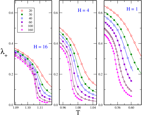
Figure 1: (Color on line) Order parameter $\lambda_{+}$ as a function of the temperature for different system widths, $H=1,4,16$ and different systems sizes, $L$. Symbols denote the result of different simulation runs, and lines represent the results of the reweighting analysis. The legends in the figures indicate the different values of $L$.

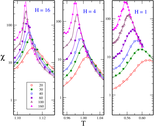
Figure 2: (Color on line) Order parameter susceptibility, $\chi$ as a function of the temperature for different system widths, $H=1,4,16$ and different systems sizes, $L$. Symbols and lines as in Fig. 1

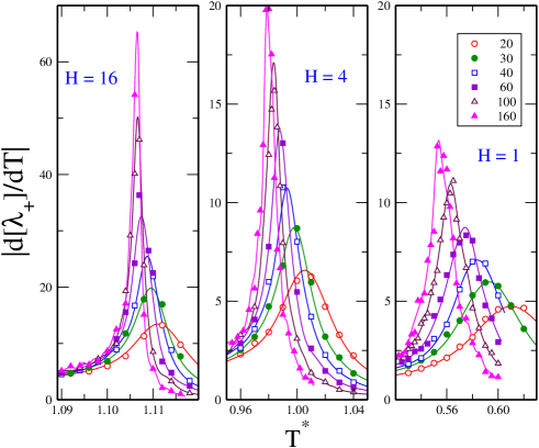
Figure 3: (Color on line) Absolute value of the derivative of the nematic order parameter with respect to the temperature, $|d\lambda_{+}/dT|$ as a function of the temperature for different system widths, $H=1,4,16$ and different systems sizes, $L$. Symbols and lines as in Fig. 1.

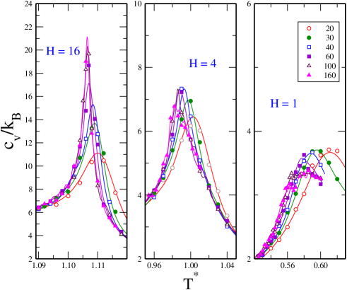
Figure 4: (Color on line) Reduced excess heat capacity as a function of the temperature for different system widths, $H=1,4,16$ and different systems sizes, $L$. Symbols and lines as in Fig. 1.

It can be seen that the dependence of these properties on $L$ is qualitatively similar for the three slit widths considered in the figures. For a given slit width, the susceptibility $\chi$ diverges with $L$ both at the temperature corresponding to the maximum and below. The curves of $<\lambda_{+}>$ as a function of $T$ exhibit an inflection point, and the derivative of $\lambda_{+}$ with respect to $T$ seems to diverge at a given critical temperature. It is to be stressed that the values of $\lambda_{+}$ below the apparent transition temperature decrease with increasing sample sizes, in contrast with the expected behavior from first and second order transitions. On the other hand the heat capacity exhibits a maximum which does not diverge with $L$. The behavior of all these properties around the transition temperature resembles that of a topological BKT transition, and it is clearly different from what one should expect in the presence of a weak first order transition. A second order transition might exhibit non-divergent heat capacity curves (with negative $\alpha$ exponent), but the decrease of $\lambda_{+}$ and divergence of $\chi$ below the pseudo-critical $T_{c}(L,H)$, fit better into the picture of a continuous phase change which shares a number of features with the continuous BKT transition. For the sake of comparison, in Figure 5 we summarize the results of simulations for unconfined systems using cubic boxes of different sizes with full PBC. It seems evident that the qualitative behavior of the confined system is quite different from that of the bulk, which is known to present a weak first order isotropic-nematic transition Priezjev .

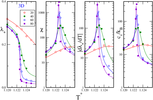
Figure 5: (Color on line) Temperature and system size dependence of various properties of the 3D LL model (cubic cells without walls). The length of the cell side, $L$, is shown in the legends. Symbols and lines as in previous figures.

Returning to the confined system, in table 1 we gather the results for the estimates of its transition temperatures for different slit widths calculated using the two aforementioned definitions of the pseudo-critical temperatures, and the two scaling laws. The results for $H=1$ agree with those reported in Ref. Kunz , but differ slightly from those reported in Ref.Mondal using the scaling laws of second order transitions. The results of the table show that the estimates of the transition temperature are conditioned by the scaling law used in the extrapolation to the thermodynamic limit. However, the results hardly depend, within error bars, on the particular definition of the pseudo-critical temperature. The variation of the transition temperature with $H$ is monotonic, and the transition temperatures approach smoothly the bulk value as $H$ increases. This is more clearly seen in Figure 6, where one can appreciate the quasi-linear dependence of $T_{c}$ (as calculated from (4)) on $1/H$. This Kelvin-like scaling of the transition temperature leads to an extrapolated value $\lim_{H\rightarrow\infty}T_{c}(H)=1.123\pm 0.005$ that agrees rather well with the bulk value $T_{c}=1.1225(1)$, which we have obtained using cubic systems with full PBC, and in accordance with the results of Priezjev and PelcovitsPriezjev . Note, however that the Kelvin scaling only applies strictly to first order phase transitions. In the case of second order transitions, correction terms must be incorporated fisher1 ; fisher2 ; vink . From our discussion it is clear that in our case a first order phase transition is ruled out, so deviations from linearity could in principle be ascribed to the continuous character of the transition. It is worth stressing that $T_{c}$ estimates become independent of the scaling relation used as $H$ increases. This is an indication, that even if the transition can still be cast into the BKT-like type for growing $H$, its scaling behavior is gradually switching to that of a regular order-disorder transition.

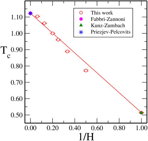
Figure 6: (Color on line) Pore width dependence of the transition temperatures estimated using the scaling law (4). The result of a linear fit to $1/H$ is represented by a solid line. Values taken from Refs.Fabbri , Priezjev , and Kunz are also included for comparison. Note that the bibliographic values and those of this work fall on top of each other and can hardly be distinguished.

We also include in Table 1 the estimates of the scaling exponent for the maximum of the susceptibility, $\gamma/\nu$, which can be drawn from the scaling relation:

$$\chi^{max}(L)\sim L^{\gamma/\nu}.$$ (6)

The results of this exponent depend on the pore width, and constitute further evidence that no first-order transition appears for the system sizes considered. One should expect in this latter instance a scaling of the type $\chi^{max}(L)\sim HL^{2}$, well away from the values obtained here for any width. Incidentally, in the $H=1$ case the value is relatively close to the two dimensional Ising critical exponentTCritPhen93 , $\gamma/\nu=7/4$, and in agreement with the value reported by Kunz and ZumbachKunz $\gamma/\nu=1.72\pm 0.05$. For larger slit widths, the value of $\gamma/\nu$ decreases, what further deviates from the limiting behavior of a first order transition when $H\rightarrow\infty$ ($\gamma/\nu=2$). This implies that in the range $0<H<\infty$ one should expect a non-monotonic behavior of $\gamma/\nu$, as was already found in the confined HSMS fluidAlmarza1 and it is a clear indication that $H=16$ is still far away from the first order transition limit. This situation is in contrast with the results recently reported by Fish and VinkFish for the generalized LL model with $p=8$. In this case the angular interaction is much narrower than that of the simple LL model and bears some resemblance with the $q$-state Potts modelDomany ; Vink07 (with $q\propto\sqrt{p}$). Fish and Vink found that $\gamma/\nu$ grows from 1.63 in the two dimensional limit approaching $\gamma/\nu\rightarrow 2$ as the critical $H_{c}$ is reached and the continuous transition develops into a first order transition. We assume that as $p$ decreases $H_{c}$ increases (as observed in Ref. Fish for $p\geq 8$), to the point that for $p=2$ the determination of the critical thickness is well beyond our present computational capabilities. On the other hand, it is to be noticed the fairly regular dependence of $T_{c}(H)$ on the pore with.

Table 1: Estimates of the isotropic-quasi-nematic transition temperature in the thermodynamic limit, using different prescription of the pseudo-critical temperatures and scaling laws (See the text for details); and scaling exponents $\gamma/\nu$ for the maxima of the susceptibility $\chi$. The transition temperature in the bulk system is $T_{N-I}=1.1225(1).$ Error bars across the table are shown between parentheses in units of the last figure and correspond to a confidence level of 95 %

H	1	2	3	4	5	8	16
$T_{c}$ [$\chi$, Eq.(4)]	0.514(2)	0.772(4)	0.889(3)	0.963(3)	1.000(2)	1.062(1)	1.104(1)
$T_{c}$ [$|d\lambda_{+}/dT|$, Eq.(4)]	0.508(4)	0.764(7)	0.889(5)	0.956(4)	0.999(3)	1.062(2)	1.104(1)
$T_{c}$ [$\chi$, Eq.(5)]	0.536(3)	0.782(3)	0.905(3)	0.973(3)	1.010(2)	1.067(1)	1.105(1)
$T_{c}$ [$|d\lambda_{+}/dT|$,Eq.(5)]	0.531(4)	0.786(5)	0.906(4)	0.969(3)	1.008(2)	1.067(1)	1.105(1)
$\gamma/\nu$	1.69(2)	1.65(3)	1.63(3)	1.59(3)	1.60(4)	1.49(3)	1.40(7)

From all this evidence, and in particular, from the size dependence of the order parameter and the susceptibility, one can conclude that the isotropic-quasi-nematic transitions found for all the confined systems under scrutiny ($1\leq H\leq 16$) do not fit in the picture of first or second order phase changes, and share some resemblance with the continuous BKT transition. The results also indicate that the possible critical thickness $H_{c}$ of the Lebwohl-Lasher model, if exists, must appear for $H_{c}>16$. Therefore, the value of $H_{c}$ reported in Ref. [cleaver, ] is most likely underestimated. It is possible to further analyze the effects of dimensionality on the transition if the walls in the $z-$direction are replaced by PBC, but still dealing with the $z$-direction on a different footing as compared with the $x-$ and $y-$ directions. More precisely, we will consider a series of systems of $L\times L\times H$ sites with PBC on all three directions and for $H=2,4,$ and 16. This anisotropic LL model is expected to enhance the correlations of the nematogen orientations in the $z-$direction, and eventually lead to the phase behavior of the bulk system as predicted by theoretical argumentsShnidman . Interestingly, we have found that the anisotropic LL model with $H=2$, and $H=4$ also exhibits BKT-like transitions similar to those of the corresponding confined LL system occurring at slightly higher temperatures. Moreover, the same behavior is found for $H=16$; the system with PBC clearly shows a dependence of $c_{v}^{max}$ with $L$ inconsistent with a first order transition. This can be appreciated in Figure 7, where we present the results for the value of the maximum of the excess heat capacity per molecule, $c_{v}^{max}$ for both systems. It can be seen that for both confined, and PBC systems $c_{v}^{max}$ does not diverge. In the same Figure we include the result for cubic systems $H=L$ with PBC (bulk LL model); in this case the expected scaling behavior, $c_{v}^{max}\sim N$, of a first-order transition is observed. From the results of $c_{v}^{max}$ it is possible to compute the latent heat, $\Delta E$ of the transitionlandau_binder :

$$c_{v}^{max}(N)=c_{\pm}+\frac{\left(\Delta E\right)^{2}}{4k_{B}T_{c}^{2}}N;$$ (7)

where $c_{\pm}$ is related with the specific heats of the two phaseslandau_binder . By fitting the results for $L\geq 25$ we get $\Delta E/\epsilon=0.0584\pm 0.0013$.

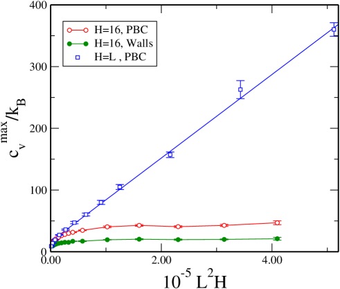
Figure 7: (Color on line) Value of the maximum of excess heat capacity per particle as a function of the system size for cubic systems (H=L) with PBC (bulk LL), systems with H=16 and PBC (anisotropic LL), and systems with H=16 confined between neutral walls. The line connecting points for the bulk system corresponds to a fit of the results to the equation $c_{v}(L)=a_{0}+a_{1}L^{3}$

In the discussion above, we have purposefully avoided an explicit reference to the questions recently raised by Paredes et al Paredes et al. (2008); Farinas as to the existence of a true BKT transition in the PLL model. After performing a finite-size scaling analysis of the simulation results at temperatures around and below the estimates of the transition temperature found in the literature, Paredes et al Paredes et al. (2008); Farinas conclude that the PLL lacks a true topological transition. Using results for several of system sizes, they infer that the $L$-dependence of the order parameter distribution for $T<T_{BKT}$ does not follow the expected scaling for a line of critical points. In particular, they argue that the lack of crossing of the Binder cumulant binder ; landau_binder ; weber curves for different system sizes at a fixed temperature is a strong evidence of the absence of quasi long range order in the PLL model. In order to gain some extra insight into this problem, we have performed series of simulations with a broad range of system sizes at three temperatures: $T^{*}=0.50$ (slightly below the range of our $T_{c}$ estimates), $T^{*}=0.54$ (slightly above), and $T^{*}=0.60$. The so-called Binder cumulant, $g_{4}$ can be defined asweber :

$$g_{4}=\frac{<\lambda_{+}^{4}>}{<\lambda_{+}^{2}>^{2}}.$$ (8)

It is well establishedlandau_binder that for second order transitions at the critical temperature $g_{4}$ reaches (for large system sizes) a critical value (different from those corresponding to ordered and disordered phases) which becomes independent on the system size, $g_{4}(L,T_{c})=g_{4}^{(c)}$. According to the usual description of the topological transitions, below $T_{BKT}$ there should be a line of critical points, and therefore at a fixed temperature $g_{4}(L;T)$ should approach a critical value $g_{4}^{c}(T)$ as $L\rightarrow\infty$. This value must be different from those of the isotropic ($g_{4}\approx 3/2$) and nematic ($g_{4}\approx 1$) phases. From this point of view one can expect that plotting $g_{4}$ as a function of $T$, the curves with different values of $L$ should merge for $T\leq T_{BKT}$. Of course, finite size effects could eventually lead to a small degree of crossing (See Ref. [Paredes et al., 2008]). Therefore, from our point of view the absence of crossing between the $g_{4}(T)$ curves with different values of $L$ must not be regarded as a signature of lack of criticality. In figures 8 and 9 we show the results of $g_{4}$ as a function of the system size for $T^{*}=0.50$ and $T^{*}=0.54$, and $T=0.60$. The results seem to be compatible with the presence of a BKT-like transition in the PLL model. For large system sizes, at $T=0.54$, and $T=0.60$ $g_{4}(L)$ seems to approach to the expected value for the isotropic phase ($g_{4}\approx 3/2$), whereas for $T=0.50$ (with system sizes up to $L=896$) the values of $g_{4}(L)$ apparently converge towards a critical value as $L\rightarrow\infty$.

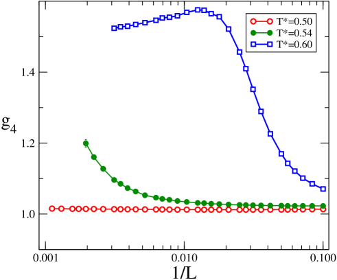
Figure 8: (Color on line) Cumulant ratio $g_{4}=<\lambda_{+}^{4}>/<\lambda_{+}^{2}>^{2}$ as a function of the inverse of the system size for $T^{*}=0.50$, $0.54$, and $0.50$

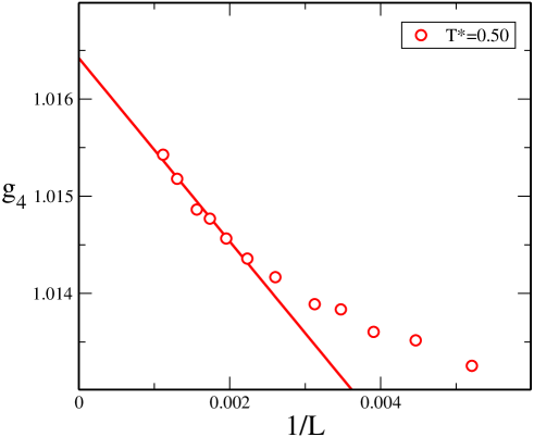
Figure 9: (Color on line) Detail of the Cumulant ratio $g_{4}=<\lambda_{+}^{4}>/<\lambda_{+}^{2}>^{2}$ as a function of the inverse of the system size for $T=0.50$

Another point raised by Paredes et al.Paredes et al. (2008) concerns the apparent violation of the hyperscaling relation of the critical exponents, $2\beta/\nu+\gamma/\nu=d$ (where $d$ is the space dimensionality). In the case of a BKT transition, the exponent $\nu$ is not defined, but the exponent ratios can still be calculatedKost . According to Ref. Paredes et al. (2008) in the case of the PLL this relation is only fulfilled within a 3% accuracy, one order of magnitude less than in the case of the XY-model. In our case, calculations carried out at $T^{*}=0.50$ (below the transition temperature) also indicate deviations around 5%, somewhat larger than the statistical uncertainties. Interestingly, previous calculations performed at the transition temperature for the continuum HSMS model Lomba et al. (2007a) agree with the hyperscaling behavior within a 0.7% error. Moreover, using an alternative definition of the susceptibility for temperatures above $T_{c}(H,L)$landau_binder ; Peczak ; Chamati

$$\chi=N<\lambda_{+}^{2}>/k_{B}T,$$

we found that the hyperscaling relation is appropriately fulfilled.

Some additional information can be obtained from an analysis of the percolation of the clusters constructed by the simulation algorithm as a function of the temperature, so as to evaluate the degree of correlation between the particle orientations within the simulated samples. Let us recall that the Swendsen-Wang-like (SW) algorithm applied in this work belong to the class of rejection-free cluster methods, and for some simple systems the temperature at which the cluster percolation occurs corresponds to that of the phase transition. This property was used by Tomita and OkabeTomita to locate the BKT transitions of two-dimensional $XY$ and Potts-Clock models in two dimensions. For the PLL model we have carried out multi-temperature simulations using the single tempering algorithm of Zhang and Mazhang . In Figure 10 we present the results of the percolation probability, $X_{per}$, defined as the fraction of configurations containing at least one percolating cluster, for the 3D LL model with PBC.

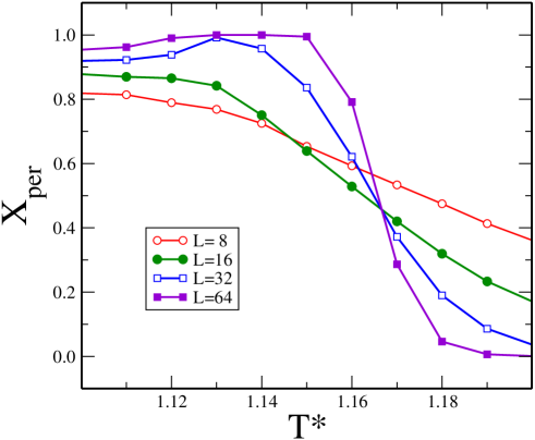
Figure 10: (Color on line) Probability of finding cluster percolation in, at least, one direction in the simulation of the three-dimensional Lebwohl-Lasher model as a function of the temperature. Different curves represent results for different system sizes.

It can be seen that the percolation threshold appears at a temperature slightly above the nematic-isotropic transition temperature. In addition. $X_{per}(L,T)$ shows a non-monotonic behavior with $T$ for large system sizes at temperatures close to the thermodynamic transition. The behavior of $X_{per}(L,T)$ is qualitatively similar for the PLL model (See Fig. 11); and at temperatures close to the $T_{BKT}$ estimates the curves for different system sizes show a clear tendency to merge. The crossing of the curves for different system sizes observed for large system size seem to indicate that the aforementioned merging is not just a consequence of correlations induced by the periodic boundary conditions. Moreover, in a similar percolation analysis carried out by us for the planar Heisenberg model (3D spins on a plane), the $X_{per}(L,T)$ curves for different system sizes do not exhibit any crossing at finite temperatures, but seemingly merge as $T\rightarrow 0$. This supports the general viewblotte that the 2D Heisenberg model does not have a phase transition at $T>0$, and underlines the essentially different phase behavior of the PLL model. In the thermodynamic limit, Figure 10 seems to indicate that in the case of the 3D LL model, there should be an abrupt change from the non-percolating state ($X_{per}=0$) to a fully percolating state ($X_{per}=1$) at a finite temperature, which fits into the picture of a first order transition between the isotropic and a truly nematic phase. In contrast, in Figure 11, one finds that in the PLL model, at least for the system sizes here considered, the fully percolating state is only reached at $T=0$. Note, that by construction, the SW cluster algorithm may yield $X_{per}<1$ for finite temperatures even in the case of truly orientationaly ordered states. The presence of the maximum after the first crossing (occurring both in the 3D LL and PLL models for finite sizes, but seemingly not present in the 3D Heisenberg system) might then well be an effect of the cluster algorithm. On the other hand, analysing the size dependence of the curves plotted in Figure 11, one is tempted to assume that the maxima will continue to grow and shift to lower T as L increases, until finally $X_{per}=1$ is reached for a given sample size. Whether this is really the case, and if so, $X_{per}=1$ is reached at $T>0$ or not, cannot be assessed at present using reasonable computer resources.

In any case, we believe that the percolation analysis sketched above confirms that the PLL model indeed presents a phase transition. It might be the case, that we are not dealing here with a strict BKT transition, if one takes into account the previous discussion on the hyperscaling relation, but its phenomenology is closely related to that of the BKT transition. On the other hand, the other anomalies in the model’s scaling behavior found by Paredes et al. Paredes et al. (2008) could be ascribed to finite size effects.

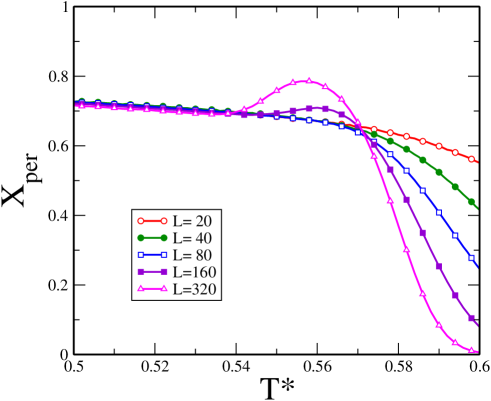
Figure 11: (Color on line) Probability of finding cluster percolation in, at least, one direction, in the simulation of the planar Lebwohl-Lasher model as a function of the temperature. Different curves represent results for different system sizes.

To conclude this discussion about the likelihood of a topological transition for the PLL model, it is worth to compare the phase behavior of the three-dimensional XY and LL models. The three-dimensional XY model presents a continuous transition campostrini without a divergence in the specific heat, whereas the three-dimensional LL model exhibits a first order transition. Taking as a reference the critical behavior of Potts models wu , we would not expect in principle that the PLL model had a weaker transition than that of the two-dimensional XY model.

In summary, we have studied the order-disorder transition for the confined LL model by means of Monte Carlo simulation and finite-size scaling analysis. Our results indicate that the critical pore width signaling the crossover between bulk and 2D behavior must be larger than the values indicated by previous simulations. The need for a reliable finite-size scaling analysis on systems with larger widths, which would imply simulations for much larger systems hampers the estimation of $H_{c}$. In addition, our results for slit-like systems with full PBC (anisotropic LL model) suggest that if $H_{c}$ has a finite value, it will likely be much larger than $H=16$. Moreover, the fact that the critical exponent relation $\gamma/\nu$ for the pore widths considered does not yet show any trend to converge towards the expected behavior in a first order transition, is a further indication that we are very likely away from the critical thickness. This might fit into the picture drawn by Telo da Gama and Tarazonatelodagama , who suggest that one should expect $H_{c}\rightarrow\infty$. However, in Ref. telodagama, it is argued that spin-waves would destroy the ordered phase for any finite $H$, but no BKT transition would occur. Our findings suggest that an order-disorder phase transition with some BKT-like features does indeed take place, as the divergence of the susceptibility, its size dependence, the crossover of percolation curves and the size dependence of the order parameter seem to evidence. It is worth pointing out that the situation depicted here is in marked contrast with the abrupt switch from continuous 2D melting behavior to discontinuous first order melting which has been argued to occur in hard sphere colloidal models when going from monolayer to bilayer systemsXu .

- (1) P. A. Lebwohl and G. Lasher, Phys. Rev. A 6, 426 (1972).
- (2) U. Fabbri and C. Zannoni, Mol. Phys. 58, 763 (1986).
- (3) Z. Zhang, O. G. Mouritsen, and M. J. Zuckermann, Phys. Rev. Lett. 69 2803(1992).
- (4) N. V. Priezjev and R. A. Pelcovits, Phys. Rev. E 63, 062702 (2001).
- (5) G. R. Luckhurst and P. Simpson, Mol. Phys. 47, 251 (1982).
- (6) G. R. Luckhurst, S. Romano, and P. Simpson, Chem. Phys. 73, 337 (1982).
- Maier and Saupe (1959) W. Maier and A. Saupe, Z. Naturforsch. 14A, 882 (1959).
- Maier and Saupe (1960) W. Maier and A. Saupe, Z. Naturforsch. 15A, 287 (1960).
- Lomba et al. (2005) E. Lomba, C. Martín, N. G. Almarza, and F. Lado, Phys. Rev. E 71, 046132 (2005).
- Lomba et al. (2006) E. Lomba, C. Martín, N. G. Almarza, and F. Lado, Phys. Rev. E 74, 021503 (2006).
- Lomba et al. (2007a) E. Lomba, N. G. Almarza, and C. Martín, Phys. Rev. E 76, 061107 (2007a).
- (12) N.G. Almarza, C. Martín, and E. Lomba, Phys. Rev E 80, 031501 (2009).
- (13) E. Mondal, and S. K. Roy, Phys. Lett. A 312, 397 (2003).
- (14) H. Kunz, and G. Zumbach, Phys. Rev. B 46, 662 (1992).
- Fariñas-Sanchez et al. (2003) A. I. Farinas-Sanchez, R. Paredes V., and B. Berche, Phys. Lett. A 308, 461 (2003).
- (16) C. Chiccoli, P. Pasini, and C. Zannoni, Physica A 148, 298 (1988).
- Paredes et al. (2008) R. ParedesV, A. I. Farinas-Sánchez, and R. Botet, Phys. Rev. E 78, 051706 (2008).
- Berezinskii (1972) V. Berezinskii, Sov. Phys.-JETP 34, 610 (1972).
- Kosterlitz and Thouless (1972) J. M. Kosterlitz and D. J. Thouless, J. Phys. C: Solid State Phys. 5, L124 (1972).
- (20) C. E. Pfister, Commun. Math. Phys. 79, 181 (1981)
- (21) A. Gelfert and W. Nolting, J. Phys.: Condens. Matter 13, R505 (2001)
- (22) D. Ioffe, S. B. Shlosman, and Y. Velenik, Commun. Math. Phys. 226, 433 (2002).
- (23) D.R. Nelson, Deffects and geometry in condensed matter physics, (Cambridge University, Cambridge, UK, 2002)
- (24) D. J. Cleaver and M. P. Allen, Mol. Phys. 80, 253 (1993).
- (25) Y. Shnidman and E. Domany, J. Phys. C 14, L773 (1981).
- (26) M. M. Telo da Gama and P. Tarazona, Phys. Rev A 41, 1149 (1990).
- (27) P. G. Ferreira, and M. M. Telo da Gama, Physica A 179, 179 (1991).
- (28) M. A. Bates, Phys. Rev. E 64, 051702 (2001).
- (29) J. M. Fish and R. L. C. Vink, Phys. Rev. E 81, 021705 (2010).
- (30) A.C.D. van Enter and S.B. Shlosman, Phys. Rev. Lett, 89, 285702 (2002).
- (31) A.C.D. van Enter and S.B. Shlosman, Commun. Math. Phys., 255, 21 (2005).
- (32) E. Domany, M. Schick, and R. H. Swendsen, Phys. Rev. Lett., 52, 1535 (1984).
- (33) H.W. J. Blöte, W. Guo, and H. J. Hilhorst, Phys. Rev. Lett., 88, 047203 (2002).
- (34) R. L. C. Vink, Phys. Rev. Lett., 98, 217801 (2007).
- (35) U. Wolff, Phys. Rev. Lett. 62, 361 (1989).
- (36) E. Lomba, C. Martín, and N. G. Almarza, Mol. Phys. 101, 1667 (2003).
- (37) R. H. Swendsen and J. S. Wang, Phys. Rev. Lett. 58, 86 (1987).
- (38) A. M. Ferrenberg and R. H. Swendsen, Phys. Rev. Lett. 63, 1195 (1989).
- (39) A. Saupe, Z. Naturforsch. A 19, 161 (1964).
- (40) M.E. Fisher and H. Nakanishi, J. Chem. Phys., 75, 5857 (1981).
- (41) H. Nakanishi and M.E. Fisher, 78, 3279 (1983).
- (42) R. L. C. Vink, A. De Virgiliis, J. Horbach, and K. Binder, Phys. Rev. E 74, 031601 (2006).
- (43) Y. Tomita and Y. Okabe, Phys. Rev. B 65, 184405 (2002).
- (44) J.J. Binney, N.J. Dowrick, A.J. Fisher, and M.E.J. Newman, The theory of critical phenomena, (Clarendon, Oxford, 1993).
- (45) D. P. Landau and K. Binder, A guide to Monte Carlo Simulations in Statistical Physics, (2nd edition) (Cambridge University Press, 2005).
- (46) A. I. Fariñas-Sánchez, R. Botet, B. Berche, and R. Paredes, arxiv:0906.4079.
- (47) K. Binder, Z. Phys. B: Condens. Matter 43, 119 (1981).
- (48) H. Weber, W. Paul, and K. Binder, Phys. Rev. E 59, 2168 (1999).
- (49) J.M. Kosterliz, J. Phys. C, 7, 1046 (1974).
- (50) P. Peczak, A. M. Ferrenberg, and D. P. Landau, Phys. Rev B 43, 6087 (1991).
- (51) H. Chamati, and S. Romano, Phys. Rev. E 77, 051704 (2008).
- (52) C. Zhang and J. Ma, Phys. Rev E 76 , 036708 (2007).
- (53) M. Campostrini, M. Hasenbusch, A. Pelissetto, P. Rossi, and E. Vicari, Phys. Rev. B 63, 214503 (2001).
- (54) F. Y. Wu, Rev. Mod. Phys. 54, 235 (1982).
- (55) X. Xu and S.A. Rice, Phys. Rev. E, 78, 011602 (2008).